Abstract
We report on studies of classical nova (CN) explosions where we follow the evolution of thermonuclear runaways (TNRs) on carbon–oxygen (CO) white dwarfs (WDs). We vary both the mass of the WD (from 0.6 M⊙ to 1.35 M⊙) and the composition of the accreted material. Our simulations are guided by the results of multidimensional studies of TNRs in WDs, which find that sufficient mixing with WD core material occurs after the TNR is well underway, and levels of enrichment are reached that agree with observations of CN ejecta abundances. We use NOVA (our one-dimensional hydrodynamic code) to accrete solar matter until the TNR is ongoing and then switch to a mixed composition (either 25% WD material and 75% solar or 50% WD material and 50% solar). Because the amount of accreted material is inversely proportional to the initial 12C abundance, by first accreting solar matter the amount of material taking part in the outburst is larger than in those simulations where we assume a mixed composition from the beginning. Our results show large enrichments of 7Be in the ejected gases, implying that CO CNe may be responsible for a significant fraction (∼100 M⊙) of the 7Li in the galaxy (∼1000 M⊙). Although the ejected gases are enriched in WD material, the WDs in these simulations eject less material than they accrete. We predict that the WD is growing in mass as a consequence of the accretion–outburst–accretion cycle, and CO CNe may be an important channel for SN Ia progenitors.
1. Introduction
Classical novae occur in close binary systems with a white dwarf (WD) primary and a secondary that is a larger, cooler star that fills its Roche Lobe. The secondary is losing material through the inner Lagrangian point, which ultimately is accreted by the WD. These binary systems are referred to as cataclysmic variables (CVs). The consequence of the WD accreting sufficient material is a thermonuclear runaway (TNR) in matter that is electron degenerate at the beginning of accretion and thus produces an event that is designated a “nova outburst” (either a classical, recurrent, or symbiotic nova, hereafter CN, RN, or SymN). While the observed outburst ejects material into the surrounding region, it does not disrupt the WD, and continued accretion implies successive outbursts. In some cases, the properties of the WD and accretion result in outbursts repeated on human timescales, which are designated RNe. If the orbital separation is large and the secondary is a red giant, then the system is designated a SymN.
Observations of the chemical composition of the gases ejected by a CN explosion show that they typically are extremely nonsolar (Warner 1995; Gehrz et al. 1998; Bode & Evans 2008; Downen et al. 2013; Starrfield et al. 2012a). Because of the CNe observations, it is assumed that the accreting material mixes with the outer layers of the WD at some time during the evolution from the beginning of accretion to the observed outburst. Thus, the observed ejected gases consist of a mixture of WD and accreted material that has been processed by hot-hydrogen burning. Canonically, it is generally assumed that the CN outburst ejects more mass (both accreted and WD matter) from the WD than that accreted from the secondary star, and, therefore, the WD is decreasing in mass as a result of continued CN outbursts and it cannot be a progenitor of a supernova of type Ia (hereafter SN Ia) outburst. In contrast, if the WD accretes more mass than it ejects during the CN outburst, then it is growing in mass and could possibly reach the Chandrasekhar limit and explode as an SN Ia.
SN Ia are the optically brightest explosions that occur in a galaxy, and they can be detected to, at least, z ∼ 2 in the universe. Studies of SN Ia show that their light curves are standardizable, allowing them to be used as distance indicators, which led to the discovery of dark energy in the universe (Riess et al. 1998; Perlmutter et al. 1999). In addition, they contribute a significant fraction of the iron-group elements to the galaxy and the solar system (Hillebrandt 2000; Leibundgut 2000). However, the systems that actually explode as SN Ia are as yet unknown. Two pathways are currently posited, the single degenerate (SD) and the double degenerate (DD). The DD scenario requires either the merging or collision of two carbon–oxygen (CO) WDs, while the SD scenario assumes that a CO WD exists in a close binary stellar system and is growing in mass toward the Chandrasekhar limit (Hillebrandt 2000; Leibundgut 2000, 2001; Maoz et al. 2014; Ruiz-Lapuente 2014; Polin et al. 2019). Therefore, the determination of the response of a CO WD to the CN phenomenon (growing or shrinking in mass) may shed light on one channel of SN Ia progenitors. In this paper, we report on our new simulations of the CN outburst and find that the WD is ejecting less mass than accreted, and, therefore, the WD is growing in mass and CO CNe could be one of the channels for the progenitors of SN Ia explosions.
Another important motivation for studies of the consequences of TNRs on CO WDs is the recent discovery of both 7Li and 7Be in the early, high-dispersion optical spectra of the material ejected from CN outbursts (Izzo et al. 2015, 2018; Tajitsu et al. 2015, 2016; Molaro et al. 2016; Selvelli et al. 2018; Wagner et al. 2018; Woodward et al. 2020), which has validated earlier predictions (Starrfield et al. 1978; Hernanz et al. 1996; José & Hernanz 1998; Yaron et al. 2005) and warrants new theoretical studies. CNe produce 7Li via a process originally described by Cameron & Fowler (1971) for red giants. Starrfield et al. (1978) then applied their mechanism to CN explosions, but that version of NOVA did not, as yet, include accretion, and they assumed that the envelope was already in place. Later, Hernanz et al. (1996) and José & Hernanz (1998) followed the accreting material and were able to investigate the formation of 7Be during the TNR. They determined the amount of 7Be carried to the surface by convection and that survived before it could be destroyed by the 7Be(p,γ)8B reaction occurring in the nuclear burning region. If it survives by being transported to cooler regions, 7Be decays via electron capture to 7Li with an ∼53 day half-life (Bahcall & Moeller 1969).
The studies reported in this paper confirm that a TNR on a CO WD overproduces 7Be with respect to solar material and in amounts that imply that such CNe are responsible for a significant amount of galactic 7Li. In contrast, 6Li is produced by spallation in the interstellar medium (Fields 2011), and its abundance in the solar system should not correlate with 7Li. Hernanz (2015) gives an excellent discussion of the cosmological importance of detecting 7Li in nova explosions. We return to this comparison in Section 5.1.
Here, we investigate both the SD scenario and the production of 7Li in the CN outburst by simulating accretion onto CO WDs, in which we include mixing of the WD outer layers with accreted solar matter after the TNR has been initiated. We report on three separate studies. First, we accrete mixed material (either 25% CO WD matter and 75% solar matter or 50% CO WD matter and 50% solar matter) from the beginning of accretion. This is the procedure used in the past for both accretion onto CO WDs and oxygen-neon (ONe) WDs (Starrfield et al. 1997, 2009, 2016; José & Hernanz 1998; Hillman et al. 2014, and references therein). However, we find, as reported later, that these explosions do not agree with the observed aspects of CNe outbursts (Warner 1995; Bode & Evans 2008; Starrfield et al. 2012a). Second, we accrete solar matter from the beginning and follow the resulting evolution through the peak and the return to nuclear burning quiescence. Third, we take the solar accretion simulations, and once the TNR is ongoing and convection extends through most of the accreted envelope ( erg gm−1 s−1), we stop the evolution and switch the accreted layers to either of the mixed compositions noted above. This last set of simulations is guided by the results of multidimensional (multi-D) studies of mixing on WDs, which indicate that sufficient material is dredged up from the outer layers of the WD during the TNR to agree with observed abundances (Casanova et al. 2011b, 2016, 2018; José 2014; José et al. 2020).
In Section 2 we describe NOVA, our one-dimensional (1D) hydrodynamic computer code. We follow that with Section 3, where we present the mixing from beginning simulations and show that they do not fit the observations. In Section 4 we present the simulations where we do not mix until near the peak of the TNR. It consists of three subsections: (1) in Section 4.1, we present simulations with only a solar mixture; (2) in Section 4.2 we present the main results of the paper in which we mix during the TNR; and (3) in Section 4.3 we discuss one simulation in detail. Section 5 gives the nucleosynthesis results. Section 6 discusses the implications of our results for the SD scenario. We end the main part of the paper with a discussion (Section 7) and conclusions (Section 8). Finally, there is an Appendix in which we demonstrate that our simulations are converged and explore the effects of our mixing technique.
2. NOVA: Our One-dimensional Hydrodynamic Code
We use NOVA (Kutter & Sparks 1972, 1974, 1980; Sparks & Kutter 1972; Starrfield et al. 2009, 2016) in this study. The most recent description of NOVA can be found in Starrfield et al. (2009, and references therein). NOVA is a 1D, fully implicit hydrodynamic computer code that has been well tested against standard problems (Kutter & Sparks 1972; Sparks & Kutter 1972). NOVA includes a large nuclear reaction network that includes 187 nuclei (up to 64Ge and including the pep reaction), the OPAL opacities (Iglesias & Rogers 1996), the Starlib nuclear reaction rates (Sallaska et al. 2013), the Timmes equations of state (Timmes & Arnett 1999; Timmes & Swesty 2000), and the nuclear reaction network solver developed by Hix & Thielemann (1999). NOVA also includes the Arnett et al. (2010) algorithm for mixing-length convection and the Potekhin electron degenerate conductivities described in Cassisi et al. (2007). These improvements have had the effect of changing the initial structures of the WDs so that they have smaller radii and, thereby, larger surface gravities compared to our previous studies. Finally, we also now include the possible effects of a binary companion (an extra source of heating at radii of ∼1011 cm) as described by MacDonald (1980), which can increase the amount of mass lost during the late stages of the outburst.
In this study, we accrete material at a rate of 1.6 × 10⁻¹⁰ M⊙ yr−1 onto complete CO WDs (the structure extends to the WD center) with masses of 0.6 M⊙, 0.8 M⊙, 1.00 M⊙, 1.15 M⊙, 1.25 M⊙, and 1.35 M⊙. We choose this value of  because it is the value used by Hernanz et al. (1996), José & Hernanz (1998), and Rukeya et al. (2017), and we compare our results to their results. It is also the value used in our study of accretion onto ONe WDs (Starrfield et al. 2009). The assumed composition of the WD outer layers is 50% 12C and 50% 16O. Studies of the evolution of low-mass stars predict that 12C
  and that this ratio varies with depth, so this can only be considered an approximate value (Althaus et al. 2010; José et al. 2016; Giammichele et al. 2018). It is the abundance of 12C that strongly affects the evolution, however, and not the C/O ratio.
The basic properties of each WD initial model (luminosity, radius, and effective temperature) are given in the first three rows of Tables 1 and 2. In contrast to our previous studies where we used 95 mass zones, we now use 150 mass zones with the zone mass decreasing from the center to the surface. The effects of increasing the number of zones on the resulting evolution are given in the Appendix. The mass of the surface zone is ∼2 × 10⁻⁹ in units of the WD mass. This is much less than either the accreted mass or the amount of core material mixed up into the envelope. This low a mass decreases the maximum time step during the accretion phase (which although implicit is tied to the mass of the outer zone), but it allows us to fully resolve the behavior of the simulations as the TNR occurs.
Table 1. Initial Parameters and Evolutionary Results for Accretion onto CO WDs: Mixing from Beginning (MFB)
| CO WD Mass (M⊙): | 0.6 | 0.8 | 1.0 | 1.15 | 1.25 | 1.35 |
|---|---|---|---|---|---|---|
| Initial: L/L⊙(10−3) | 4.8 | 4.8 | 4.9 | 4.7 | 4.8 | 5.5 |
| Initial: R(103 km) | 8.5 | 6.8 | 5.3 | 4.2 | 3.4 | 2.3 |
| Initial: Tc(107 K) | 1.9 | 1.7 | 1.6 | 1.5 | 1.5 | 1.5 |
| Initial: ρc (107 gm cm−3) | 0.34 | 0.95 | 2.9 | 8.3 | 21.0 | 87.0 |
| Initial: Teff(104 K) | 1.4 | 1.5 | 1.7 | 2.0 | 2.2 | 2.7 |
| 25% White Dwarf–75% Solar | ||||||
| τacc(105 yr) | 9.8 | 3.8 | 2.0 | 1.0 | 0.6 | 0.2 |
| Macc(10−5M⊙) | 15.5 | 6.0 | 3.1 | 1.7 | 0.9 | 0.3 |
| Tpeak(108 K) | 1.2 | 1.4 | 1.7 | 2.0 | 2.3 | 2.6 |
| 0.014 | 0.041 | 0.20 | 0.89 | 2.4 | 6.1 | |
| Lpeak/L⊙ (104) | 4.6 | 4.6 | 4.4 | 7.7 | 4.8 | 7.0 |
| Teff-peak(105 K) | 1.1 | 3.0 | 3.4 | 5.7 | 8.1 | 11.0 |
| Mej(10−7M⊙) | 8.0 | 3.7 | 0.15 | 0.98 | 0.33 | 0.62 |
| N(7Li/H)ej/N(7Li/H)⊙ | 22.0 | 1.1 × 10² | 1.8 × 10² | 7.9 × 10² | 1.4 × 10³ | 2.6 × 10³ |
| Mej/Macc(%) | 0.5 | 0.6 | 0.05 | 0.6 | 0.4 | 2.0 |
| Vmax(102 km s−1) | 3.9 | 3.6 | 4.1 | 4.6 | 4.3 | 5.7 |
| 50% White Dwarf–50% Solar | ||||||
| τacc(105 yr) | 6.1 | 3.2 | 1.6 | 0.8 | 0.5 | 0.2 |
| Macc(10−5M⊙) | 9.7 | 5.0 | 2.5 | 1.3 | 0.7 | 0.2 |
| Tpeak(108 K) | 1.1 | 1.4 | 1.7 | 2.0 | 2.2 | 2.6 |
| 0.015 | 0.081 | 0.33 | 1.4 | 4.3 | 17.0 | |
| Lpeak/L⊙ (104) | 2.6 | 7.3 | 3.2 | 8.4 | 8.1 | 11.5 |
| Teff-peak(105 K) | 2.0 | 3.6 | 4.4 | 6.5 | 8.6 | 11.7 |
| Mej(10−7M⊙) | 16.0 | 4.1 | 0.44 | 1.3 | 0.83 | 4.0 |
| N(7Li/H)ej/N(7Li/H)⊙ | 44.0 | 1.4 × 10² | 2.9 × 10² | 9.6 × 10² | 1.4 × 10³ | 4.3 × 10³ |
| Mej/Macc(%) | 1.6 | 0.8 | 0.2 | 1.0 | 1.2 | 20 |
| Vmax(102 km s−1) | 0.7 | 3.6 | 5.9 | 12.9 | 14.9 | 19.4 |
Download table as: ASCIITypeset image
Table 2. Initial Parameters and Evolutionary Results for Accretion onto CO WDs: Mixing during the Thermonuclear Runaway (MDTNR)
| CO WD Mass (M⊙): | 0.6 | 0.8 | 1.0 | 1.15 | 1.25 | 1.35 |
| Initial: L/L⊙(10−3) | 4.8 | 4.8 | 4.9 | 4.7 | 4.8 | 5.5 |
| Initial: R(103 km) | 8.5 | 6.8 | 5.3 | 4.2 | 3.4 | 2.3 |
| Initial: Teff(104 K) | 1.4 | 1.6 | 1.8 | 2.0 | 2.2 | 2.7 |
| τacc(105 yr) | 19.8 | 9.9 | 5.1 | 2.4 | 1.6 | 0.6 |
| Macc(10−5M⊙) | 31.4 | 16.0 | 8.1 | 3.9 | 2.6 | 1.0 |
| Solar Mixture | ||||||
| Tpeak(108 K) | 1.2 | 1.6 | 2.0 | 2.3 | 2.6 | 3.0 |
| 0.032 | 0.73 | 1.6 | 1.8 | 1.6 | 1.8 | |
| Lpeak/L⊙ (104) | 3.9 | 3.8 | 2.1 | 2.7 | 3.2 | 10.8 |
| Teff-peak(105 K) | 0.9 | 1.6 | 2.0 | 3.4 | 5.3 | 7.7 |
| Mej(10−7M⊙) | 6.8 | 12.0 | 0.034 | 0.33 | 0.0 | 0.36 |
| N(7Li/H)ej/N(7Li/H)⊙ | 1.0 × 10⁻⁵ | 1.4 × 10⁻⁵ | 1.5 × 10⁻² | 4.7 × 10⁻³ | 4.6 × 10⁻⁴ | 6.2 × 10⁻³ |
| Mej/Macc(%) | 0.2 | 0.8 | ∼0.0 | ∼0.0 | 0.0 | 0.4 |
| Vmax(102 km s−1) | 3.6 | 4.5 | 3.8 | 5.1 | 0.0 | 4.7 |
| 25% White Dwarf–75% Solar | ||||||
| Tpeak(108 K) | 1.3 | 1.7 | 2.0 | 2.4 | 2.8 | 3.4 |
| 0.66 | 0.65 | 1.2 | 3.4 | 11.4 | 34.3 | |
| Lpeak/L⊙ (105) | 0.7 | 1.8 | 2.8 | 2.3 | 3.3 | 5.9 |
| Teff- peak(105 K) | 1.1 | 2.4 | 3.2 | 8.4 | 8.0 | 10.5 |
| Mej(10−6M⊙) | 0.49 | 2.9 | 4.3 | 12.8 | 20.8 | 5.0 |
| N(7Li/H)ej/N(7Li/H)⊙ | 78.0 | 5.0 × 10² | 1.6 × 10³ | 2.8 × 10³ | 3.0 × 10³ | 3.5 × 10³ |
| Mej/Macc(%) | 0.2 | 2 | 5 | 33 | 80 | 48 |
| Vmax(103 km s−1) | 0.4 | 1.4 | 2.8 | 2.8 | 3.4 | 1.4 |
| 50% White Dwarf–50% Solar | ||||||
| Tpeak(108 K) | 1.4 | 1.8 | 2.2 | 2.5 | 3.4 | 4.5 |
| 0.012 | 0.085 | 0.47 | 1.7 | 26.0 | 600.0 | |
| Lpeak/L⊙ (106) | 3.0 | 2.6 | 3.4 | 2.0 | 2.7 | 6.5 |
| Teff-peak(105 K) | 1.5 | 3.2 | 4.2 | 8.3 | 8.3 | 49.0 |
| Mej(10−5M⊙) | 16.0 | 11.0 | 6.3 | 3.4 | 2.3 | 0.9 |
| N(7Li/H)ej/N(7Li/H)⊙ | 1.9 × 10² | 7.4 × 10² | 1.6 × 10³ | 2.8 × 10³ | 3.6 × 10³ | 3.4 × 10³ |
| Mej/Macc(%) | 51 | 69 | 78 | 87 | 90 | 88 |
| Vmax(103 km s−1) | 2.5 | 4.3 | 6.4 | 6.6 | 6.5 | 7.6 |
Download table as: ASCIITypeset image
As described in Starrfield et al. (2009, and references therein), we begin with a complete WD in which the core composition extends to the surface. We accrete onto this WD at the chosen rate, held constant through the accretion phase, until we reach a peak nuclear reaction rate in the envelope of 1011 erg gm−1 s−1. At this point in the evolution, we stop accreting and NOVA evolves the simulation through the peak of the TNR and the following decline in temperature toward quiescence. It follows the evolution of the expanding outer layers and determines if they are ejected. This value of the nuclear reaction rate was chosen to allow us to accrete as much material as possible and then stop when the envelope is nearly completely convective. We tabulate, as the ejected mass, the amount of material that is expanding at speeds above the escape velocity and also has become optically thin. We do not remove any mass zones during the evolution as this reduces the numerical pressure on the zones below, causing them to accelerate outward and also reach escape speeds. We find that even if the material is ejected, we can follow the mass zones until they have reached radii of a few times 1012 cm. At these radii, the density in the outer layers has fallen to values that are now below the lower limit of the physics (opacity, pressure equation of state, energy equation of state) tables (ρ < 10−12 gm cm−3), and we end the evolution.
Finally, although it is commonly assumed that a CO WD should not have a mass exceeding ∼1.15M⊙ (Iben 1991; Ritossa et al. 1996; Iben et al. 1997), as we report in this paper our simulations suggest that WDs are growing in mass, so there should be massive CO WDs in CN systems. An example of this class is nova LMC 1991, a CO nova, which exhibited a super Eddington luminosity for more than 2 weeks (Schwarz et al. 2001), likely requiring a WD mass exceeding ≃1.35M⊙. Moreover, the WDs in four of the nearest CVs (U Gem: 1.2 M⊙ (Echevarría et al. 2007), SS Cyg: 0.8 M⊙ (Sion et al. 2010), IP Peg: 1.16 M⊙ (Copperwheat et al. 2010), and Z Cam: 0.99 M⊙ (Shafter 1983)) are more massive than the canonical value for single WDs of 0.6 M⊙ (Sion 1986). More recently, Sion et al. (2019) reported a WD mass for the RN CI Aql of 0.98 M⊙, Shara et al. (2018) report that the mean WD mass for 82 Galactic CNe is 1.13 M⊙ and 10 RNe is 1.31 M⊙, while Selvelli & Gilmozzi (2019) analyzed 18 old novae, using data from both IUE and Gaia, and report that many WDs in CNe have masses above the canonical value for single WDs.
3. Simulations with a Mixed Composition from the Beginning
The principal motivation for this paper is to present a new set of simulations where we do not assume a mixed composition until the TNR is well underway. However, in order to demonstrate that there is a need for this technique, we first present the results of new simulations where we “mix from the beginning” (hereafter MFB), as has been done in nova simulations for many years (Starrfield et al. 2016, and references therein). This technique was used because there was no consensus on how WD core matter was mixed into the accreted envelope, although the observations of both fast CO and ONe CNe required that such mixing occur (Gehrz et al. 1998; Downen et al. 2013; Starrfield et al. 2016, and references therein). Nevertheless, it is not physically reasonable to assume the accreted matter is fully mixed from the beginning of accretion. A discussion of mixing mechanisms can be found in José et al. (2007).
We find that none of these MFB simulations eject sufficient material to agree with the observations, and for those that do eject some material, the expanding gases have too low a velocity. This same result was also found in an earlier study of accretion onto CO WDs (Starrfield et al. 1997). In contrast, our previous ONe CNe simulations (Starrfield et al. 2009), which used the MFB technique, did eject significant material because they were initiated with a far lower value for the initial abundance of 12C and more material was accreted prior to the TNR than in the CO simulations.
We use two different mixed compositions in this study. The first is what we used in Starrfield et al. (1997) and is 50% CO WD matter and 50% solar matter (Lodders 2003). The second composition is 25% CO WD matter and 75% solar in order to better compare our results with Hernanz et al. (1996), José & Hernanz (1998), and Rukeya et al. (2017), who also investigated the consequences of 25% CO WD matter and 75% solar matter. In addition, Kelly et al. (2013) studied abundances in ONe novae and reported that the 25% WD–75% solar mixture was a better fit to the observations.
The initial conditions and evolutionary results for the MFB simulations are given in Table 1. The columns are the values for each of the CO WD masses listed in the top row in solar mass. The first rows give the initial luminosity, radius, central temperature, central density, and effective temperature for each of the WD masses prior to accretion. As expected, as the WD mass increases, its radius decreases, which is a result of electron degeneracy. We choose an initial luminosity of ∼4 × 10⁻³ L⊙ in order to obtain as large an amount of accreted mass as possible. This luminosity is the same value as used in our ONe study (Starrfield et al. 2009). Since it is virtually the same initial luminosity for all of the WD masses, as the radius decreases, the initial Teff must increase. The decrease in radius, in turn, increases the gravitational potential energy at the surface, and the TNR is reached with a smaller amount of accreted mass and, thereby, a smaller accretion time.
These effects can be seen in the next set of rows, which give the evolutionary results for the first mixture, which is 25% WD matter and 75% solar matter (Lodders 2003). The model composition is noted in bold. The rows are the accretion time to the beginning of the TNR, τacc, and Macc, the total accreted mass. The next set of rows tabulate, as a function of WD mass, the peak temperature in the simulation (Tpeak) with the scaling factor in parentheses for all rows, the peak rate of energy generation (nuc-peak), the peak surface luminosity in units of the solar luminosity (Lpeak/L⊙), the peak effective temperature (Teff-peak), the amount of mass ejected in solar masses (Mej), the amount of 7Li ejected with respect to the solar value, where we have assumed that all of the 7Be produced in the TNR will decay to 7Li (N(7Li/H)ej/N(7Li/H)⊙), the ratio of the ejected mass to accreted mass in percent (Mej/Macc), and the velocity of the surface zone, which is the maximum velocity in each simulation (Vmax). We express the 7Li results in the same ratio as given by Hernanz et al. (1996, Table 1) in order to provide a direct comparison (see Section 5.1). We use the Anders & Grevesse (1989) value for N(7Li/H)⊙ of 2.04 × 10⁻⁹ only in the table to assist in the comparison with Hernanz et al. (1996) because that is the value they used. In our simulations, however, we use the more modern value from Lodders (2003) meteoritic abundances. The actual value does not matter in the simulations, however, because all of the initial 7Li is destroyed during the TNR.
In Section 5.1 (Table 3) we compare our 7Li and ejecta mass predictions with those of Hernanz et al. (1996), José & Hernanz (1998), and Rukeya et al. (2017), who also mixed from the beginning. In Section 5.1, we also discuss the differences and agreements between our three studies.
In the following rows, we tabulate exactly the same information but for the MFB simulations with 50% WD and 50% solar matter. Because of the increase in initial 12C abundance, once the accreting material gets sufficiently hot for CNO burning rather than the initial p − p chain, which now includes the pep reaction  as discussed in Starrfield et al. (2009), the increased energy generation per unit accreted mass reduces the time to the TNR and the amount of accreted mass. Interestingly, the peak temperature during the TNR is roughly the same for both mixtures. However, the peak rate of energy generation is considerably higher in the 50% WD–50% solar mixture because of the increased 12C abundance. The remaining evolutionary parameters are also higher for the 50% WD–50% solar mixture. The most material ejected at the highest velocities occurs for the 50% WD–50% solar simulation on the 1.35 M⊙ WD. However, the amount of ejected mass, 4.0 × 10⁻⁷M⊙, is far lower than the typical ejecta mass estimates for CNe and so are the associated ejecta velocities (Warner 1995; Gehrz et al. 1998; Bode & Evans 2008; Starrfield et al. 2012a).
In the first three figures, we plot the evolutionary results for the MFB simulations. The top panel of Figure 1 shows the variation of temperature with time for the zone where peak conditions occur for all six CO WD masses. Our composition for these simulations is 25% WD–75% solar matter, identified on the plot as 25_75 MFB. The WD mass is identified in the legend on the figure. We use the same line identifiers for WD mass in all plots in this paper. As expected, the most massive WD reaches the highest peak temperature. We have offset each evolutionary sequence in time so as to clearly show the rise to maximum temperature and decline. The time axis is chosen to emphasize the major features in the evolution of each of the WD simulations. Peak temperature is reached a few hundred seconds after the increasing temperature exceeds 108 K. The rise in temperature ends when virtually all of the light nuclei in the convective region have become positron-decay nuclei (13N, 14O, 15O, and 17F), and no further proton captures can occur on 14O and 15O until they have decayed (Starrfield et al. 1972, 2016). The simulation for the 0.6 M⊙ WD shows that the temperature has just reached the peak after 8000 s of evolution. We follow each of the simulations through peak temperature and its decline to values where no further nuclear burning is occurring in the outer layers.
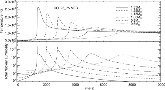
Figure 1. Top panel: variation with time of the temperature in those mass zones near the interface between the outer layers of the CO WD and the accreted plus WD matter for the simulations with 25% WD material and 75% solar material. In these simulations, we accreted the mixed composition from the beginning (MFB). The results for all six simulations are shown (the WD mass is identified in the legend). The curve for each sequence has been shifted in time to improve its visibility. As expected, the peak temperature achieved in each simulation is an increasing function of WD mass. Bottom panel: variation with time of the total nuclear luminosity (erg s−1) in solar units (L⊙) around the time of peak temperature during the TNR. We integrated over all zones with ongoing nuclear fusion to obtain the plotted numbers. The identification with each WD mass is given on the plot, and the evolution time has again been shifted to improve visibility. The cause of the sharp spike at the peak of the curve is discussed in the text.
Download figure:
Standard image High-resolution imageFigure 2 shows the same two plots as in Figure 1 but for the composition with 50% WD matter and 50% solar matter (50_50 MFB in the plots). There is a difference between the time axes in Figures 1 and 2. As seen for both compositions, not only is the peak temperature an increasing function of WD mass, but the rise and decay times are also functions of WD mass. For example, in Figure 2, the rise time for the 1.35 M⊙ WD is tens of seconds, while that for the 0.6 M⊙ WD is more than 4000 s.
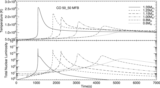
Figure 2. Top panel: the same plot as in Figure 1 but for the simulations with 50% WD matter and 50% solar matter and mixed from the beginning (MFB). While there is significantly more 12C in these simulations than in the 25%–75% simulations, the increased energy production, once the CNO reactions have become important, results in less accreted mass and a smaller peak temperature. Again, we have shifted the curves in time to improve their visibility. Bottom panel: the same plot as shown in the bottom of Figure 1 but for the simulations with 50% WD matter and 50% solar. The small “glitch” in the 1.35 M⊙ sequence at a time of ∼2100 s is caused by a change in the spatial distribution of the convective region.
Download figure:
Standard image High-resolution imageThe bottom panels of both Figures 1 and 2 show the evolution of the total nuclear luminosity (in units of the solar luminosity) as a function of time for each composition. Again, the rise time for the most massive WDs is much shorter than for the lower mass WDs. Clearly, however, for these two compositions, the peak nuclear energy generation is nearly the same for the most massive WDs. The nuclear energy in the 50% WD–50% solar simulations declines faster than in the 25% WD–75% solar simulations because the ejection velocities are larger and the temperatures are dropping more rapidly. The sharp spike is characteristic of all our enriched carbon simulations. There is a steep rise to maximum nuclear luminosity as the expanding convective region encompasses more of the accreted layers, carrying the β+-unstable nuclei to the surface. In addition, at peak temperature, most of the CNO nuclei in the envelope are now β+-unstable nuclei, and any further rise in nuclear luminosity depends on these nuclei decaying. Their decay at the surface causes the peak energy generation in the surface mass zones to exceed 1014 erg gm−1 s−1 and results in an immediate expansion of the WD outer layers.
In Figure 3 we show the initial evolution of the bolometric magnitude as a function of time for both mixtures. The rapid rise to maximum is caused by the intense heat from the decays of the β+-unstable nuclei that have reached the surface on the convective turnover time (∼200 s). In contrast, the absolute visual magnitudes (not shown in order to prevent clutter) for these simulations climb slowly in time as the expanding surface layers cool to ∼104 K. The outermost zones reach this temperature when the surface radii have expanded to about 1012 cm, and we end the evolution. At this time, the outermost layers have become optically thin and, if they have reached escape velocity, are expanding ballistically. We do not follow the simulations longer because the density in these layers has dropped below ∼10−12 gm cm−3.
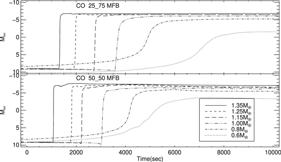
Figure 3. Top panel: variation with time of the absolute bolometric magnitude for the simulations where we mixed a composition of 25% WD matter and 75% solar from the beginning (MFB). While the simulations on the more massive CO WDs reach values that agree with observations, those on the lower mass WDs are too faint to agree with the observations. Bottom panel: the same plot as in the top panel but for a mixed composition of 50% WD matter and 50% solar matter. Again the simulations on lower mass CO WDs do not reach values that agree with typical CN observations where MBol is around −7 or higher. The small variations are real and suggest oscillatory behavior in the light curves, but these times are normally before the nova is discovered.
Download figure:
Standard image High-resolution imageAttempts to predict the evolution of the light curve at later times typically use the Rosseland mean, which is a transparency mean (1/opacity) combined with a blackbody source function. However, the atmospheres of CNe after maximum do not resemble blackbodies.
We end this section by emphasizing that a key parameter affecting the evolution is the initial 12C abundance in the accreted material (Hernanz et al. 1996). This nucleus is a catalyst in the CNO cycle, and the MFB prescription implies a much higher initial 12C concentration than starting the simulation with just a solar composition. By increasing the amount of 12C with respect to hydrogen, once the CNO cycle becomes important, the rate of energy production is increased, and the temperature in the nuclear burning region increases rapidly to the peak of the TNR. Thus, less mass is accreted than if the mixture had a solar composition (this is shown in Section 4.1). Reducing the amount of accreted mass at the time of peak temperature in the nuclear burning region results in a lower density and temperature and, thereby, less degeneracy. If the material is less degenerate, then it expands earlier in the TNR and, in combination with the formation of the β+-unstable nuclei, halts the rising temperature. Since the peak temperature is lower, the peak rate of energy generation is lower, causing the total amount of energy produced during the TNR to be smaller. In consequence, too little mass is ejected, at too low velocities, and the properties of the simulations do not resemble typical CNe or RNe observations (Warner 1995; Bode & Evans 2008; Starrfield et al. 2012a).
4. Simulations with the Composition Mixed during the Thermonuclear Runaway
As already emphasized, the treatment of the composition of the accreted material has changed in this study compared to our prior work. In our last study, we assumed that the mixing of WD and accreted material occurred from the beginning of the simulation and only used a composition of 50% WD (ONe) and 50% solar material (Starrfield et al. 2009). We began this study using this procedure but assumed a CO composition and found as reported both in Section 3 and previously in Starrfield et al. (1997, for a CO composition) that the results (ejected mass and ejecta velocities) were too small to agree with the observations.
In order to increase the amount of accreted material, therefore, we now use the results of multidimensional simulations as guides. These studies show that sufficient material is dredged up into the accreted envelope from the outer layers of the WD by convectively associated instabilities when the TNR is well underway (Casanova et al. 2010, 2011b, 2016, 2018; José 2014; José et al. 2020). We simulate their calculations by first accreting a solar mixture (Lodders 2003) until the peak energy generation in the nuclear burning region exceeds 1011 erg gm−1 s−1 and ∼96% of the accreted material is convective (see the Appendix). At this time, we switch the composition of the accreted layers to a mixed composition (both abundances and the associated equations of state and opacities) and subsequently evolve the simulation through peak temperature and decline. It typically takes NOVA less than ∼2 s of “star” time (but many time steps) to adjust to the new composition. A similar technique has already been used by José et al. (2007) in their study of the “First Nova Explosions.” They explored a variety of timescales for mixing the WD material into the accreted layers, once convection was underway, and found that using short timescales was warranted. More recently, José et al. (2020) have expanded their earlier studies by using both 1D and multi-D codes to explore this technique and its effect on CN explosions. They choose a temperature of 108 K to make the switch from 1D to multi-D based on the multi-D study of Glasner et al. (2007), who explored switching for temperatures between 5 × 10⁷ and 9 × 10⁷ K. Our chosen energy generation (for the various WD masses in this study) is equivalent to temperatures of ∼6 × 10⁷ K and a convective region that spans almost the entire accreted envelope.
4.1. Solar Accretion
In this subsection, we present the evolution of just the solar accretion phase of the study. We then follow that with subsections describing the simulations assuming the mixed compositions. The initial conditions and evolutionary results are presented in Table 2. The variables in the tables are the same as already described for Table 1. The initial conditions for each of the six CO WD masses are given in the first three rows. The values in these rows are identical to the first three rows in Table 1 and are repeated here only for consistency. The next two rows give the accretion time to the beginning of the TNR, τacc, and Macc is the total accreted mass at that time. These values are those used both for the solar accretion simulations and, later, for the two mixed composition simulations for each of the listed WD masses (Section 4). We begin each of the sets of simulations with the composition listed in bold. As in the MFB simulations, we use 150 mass zones, with the mass of the zone decreasing outward in radius, and accrete at 1.6 × 10⁻¹⁰M⊙ yr−1.
We can see the immediate effects of accreting a solar composition instead of a mixed composition. Comparing the results given in Table 2 to those in Table 1, we see that the reduced amount of 12C in the solar accretion simulations significantly increases the amount of accreted mass. For example, comparing the solar accretion simulation to the 25% WD–75% solar (MFB) simulation, we find that about twice as much mass is accreted at 0.6 M⊙ and a factor of 3 times more mass at 1.35 M⊙. The peak temperature is higher for all WD masses in the solar accretion simulation as compared to the MFB simulations. The increased mass and degeneracy at the bottom of the accreted material clearly compensate for the larger amount of 12C in the MFB simulations.
Figure 4 (top panel) shows the evolution of the temperature with time for the zones where peak conditions in the TNR occur for all of the CO WD masses accreting just a solar composition. Although there is more accreted mass in each of the simulations, the temperature evolution is extremely slow, as shown by the time axis. While the 1.35M⊙ simulation takes ∼2 × 10⁴ s to evolve through the peak and decline of the TNR, the 0.6M⊙ simulation is still on the rise after ∼5 × 10⁴ s. In contrast, the equivalent MFB simulations take a far shorter time (shown in Figures 1 and 2) to evolve through the peak, as do the simulations to be reported on in the next subsection.
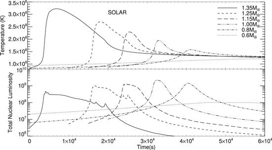
Figure 4. Top panel: the same plot as in Figure 1 but for the simulations with accretion of only solar material. These simulations are used to determine the amount of mass accreted before switching to a mixed composition. Nevertheless, we follow them through the explosion. The time axis is much longer than for any of the other simulations because of the slow evolution of these sequences. Note that the 0.6 M⊙ simulation has not yet reached peak temperature after 5 × 10⁴ s of evolution, although it started from the same beginning temperature as the simulations for other CO WD masses. Bottom panel: the same plot as shown in the bottom panel of Figure 1 but for the simulations that accrete only solar matter and are assumed not to have mixed with WD matter. The “glitches” seen in the more massive WD evolution are caused by the convective region changing its spatial distribution, with respect to the mass zones, as the material expands. Unlike all the other simulations, the total energy increases as the WD mass decreases. This is because the accreted mass has declined with increasing WD mass and there is less material involved in the evolution. In contrast, both peak temperature and peak energy generation do increase with increasing CO WD mass, as is shown in Table 2.
Download figure:
Standard image High-resolution imageFigure 4 (bottom panel) shows the variation in total nuclear energy generation around the peak of the TNR. It should be compared with the bottom panels in Figures 1 and 2. The rise to peak nuclear energy generation is extremely slow, and the decline is also slow. In addition, the peak is more than a factor of 10 lower than in the MFB simulations for the same WD mass. The “glitches” seen in the more massive WD evolution are caused by the convective region changing its spatial distribution, with respect to the mass zones, as the material expands. Unlike all the other simulations, the total energy as a function of time increases as the WD mass decreases. This is because the total accreted mass has declined with increasing WD mass and there is less material involved in the evolution. However, both peak temperature and peak energy generation do increase with increasing CO WD mass, as is shown in Table 2.
Figure 5 is the solar accretion analog of Figure 3, showing the time evolution of the bolometric magnitude for the solar accretion simulations. Peak  is an increasing function of WD mass, but even the simulation on the most massive WD does not reach values that are observed in a typical CN outburst of ∼−8. These, however, might fit some of the slowest and faintest CNe shown in Kasliwal et al. (2011).
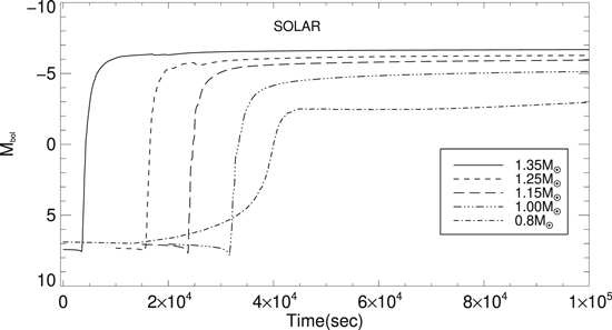
Figure 5. The same plot as shown in Figure 3 but for the solar composition simulations. Note that only the simulations on the most massive CO WDs reach peak values close to those that are observed. They also evolve extremely slowly compared to the mixed compositions (both MFB and MDTNR), as can be seen on the time axis. We do not plot the evolution of the 0.6 M⊙ simulation because it is still rising after 105 s.
Download figure:
Standard image High-resolution imageFinally, we note that the consequences of accretion of solar material onto WDs with a larger variation in mass and mass accretion rates, and where no mixing of WD with accreted material was assumed, have been published elsewhere (Starrfield et al. 2012a, 2012b; Newsham et al. 2014). They found that a TNR occurred for all WD masses and mass accretion rates.
4.2. Simulations Using Compositions Mixed during the TNR
We now take the results for each CO WD mass from the evolution reported in the last subsection and switch to a mixed composition when the peak energy generation in the simulation has reached 1011 erg gm−1 s−1. At this value, convection is well underway, and the convective region extends almost to the surface, as discussed in the Appendix. Once we have switched the composition, we continue the evolution, without assuming any further accretion, through peak temperature of the TNR and the following decline in temperature to where there is no further nuclear burning in the outer layers. We use the same two mixtures (either 25% CO WD and 75% solar material or 50% CO WD and 50% solar material) as used in the MFB simulations. These two sets of simulations are identified on the plots as either 25_75 Mixing During the TNR (25_75 MDTNR) or 50_50 Mixing During the TNR (50_50 MDTNR).
We emphasize that the same initial model (thermal structure, spatial structure, and amount of accreted mass distributed through the same number of mass zones) is used for the two sets of simulations at the time we switch to a mixed composition. The violence of the resulting evolution now depends on the amount of 12C in the accreted layers (solar plus WD) after the switch in composition. Because the pressure and density are unchanged by the switch in composition, increasing the 12C abundance changes the mean molecular weight, μ, which increases the temperature and, thereby, the rate of energy generation. The simulations now evolve much more rapidly and reach higher peak values than the equivalent MFB or solar simulation (for the same WD mass and mixed composition). This result is in contrast to the previously described MFB accretion phases (Section 3), where a higher initial 12C abundance resulted in a weaker explosion. Peak temperature is reached about 100 seconds after the temperature exceeds 108 K. The rise in temperature ends because virtually all of the CNO nuclei in the convective region have become positron-decay nuclei.
We follow each of the simulations through peak nuclear burning, peak temperature, and decline. We end the simulation when the outer layers have reached radii of a few ×1012 cm. At this radius, they have started to become optically thin and, in some of the simulations, the material has reached escape velocity and the density has declined to below ∼10−12 gm cm−3.
As discussed in the last subsection, the first set of evolutionary results in Table 2 shows the consequences of following the solar accretion simulation through the TNR, without any mixing, and its return to near quiescence. The next two sets of rows provide exactly the same information but for the mixed composition simulations with 25% CO WD and 75% solar matter, and followed below by the results for the 50% CO WD and 50% solar matter simulations. Comparing the 25% WD–75% solar MDTNR simulations to the 50% WD–50% solar MDTNR simulations, the large enrichment of 12C in the simulations with more WD matter causes a more extreme set of evolutionary results.
The plots of temperature versus time for these two sets of simulations are given in Figures 6 and 7. Both the vertical and horizontal scales in these two figures are different. As noted before, the peak temperature during the TNR is an increasing function of WD mass. The simulation with 25% WD–75% solar MDTNR involving a CO WD with a mass of 1.35 M⊙ reaches the highest temperature of 3.4 × 10⁸ K, while the simulation on the lowest mass WD, 0.6 M⊙, reaches the lowest peak temperature of 1.3 × 10⁸ K (Figure 6). Comparing these values to the results for the 50% WD–50% solar MDTNR simulations, we find that there is hardly any difference in peak temperature and energy generation for the lower mass WDs, but the values for the 1.25 M⊙ and 1.35 M⊙ simulations are far larger for the more carbon-enriched simulation (see Tables 2 and 7).
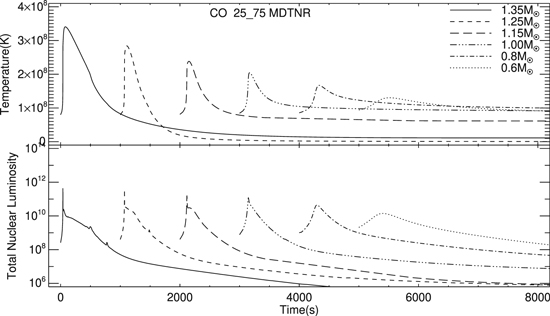
Figure 6. Top panel: variation with time of the temperature in those mass zones near the interface between the outer layers of the WD and the accreted plus WD matter for the simulations with 25% WD material and 75% solar. This plot is the analog of the top panel of Figure 1. The results for all six simulations are shown (the WD mass is identified in the inset). The curve for each sequence has been shifted in time to improve its visibility. As expected, the peak temperature achieved in each simulation is an increasing function of CO WD mass. Bottom panel: same as the bottom panel of Figure 1 but for the simulation with 25% WD–75% solar. The small “glitches” that appear on the decline are caused by convection moving in and out and bringing in small amounts of fresh nuclei to the nuclear burning regime.
Download figure:
Standard image High-resolution image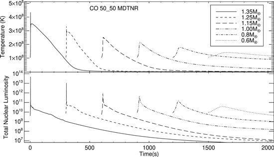
Figure 7. Top panel: same as Figure 6 but for the simulations with 50% WD matter and 50% accreted matter. Because of the increased 12C, the rate of energy generation is larger for a given temperature and density, and these simulations evolve much more rapidly than the simulations with a lower 12C abundance. Therefore, the evolution time for this series of sequences is significantly shorter than that in Figure 6. The extremely rapid increase and decrease in temperature indicate that the simulation formed a shock wave in the zone where peak temperature occurred. Bottom panel: the same plot as in Figure 6 but for the simulation with 50% WD matter and 50% accreted matter. The horizontal and vertical axes differ in these two plots. Because of the much larger amount of 12C in these simulations, the evolution is more extreme and faster than for those simulations with a smaller amount of 12C.
Download figure:
Standard image High-resolution imageThe peak temperature for the 1.35 M⊙ 50% WD–50% solar MDTNR simulation reaches 4.5 × 10⁸ K, and the peak rate of energy generation is 6.0 × 10¹⁹ erg gm−1 s−1 in the region closest to the interface between the WD core and accreted plus core material. The rise in temperature for this sequence is so rapid that a shock forms at the interface between the accreted and WD matter and moves through the envelope in seconds. The consequences of the shock can be seen in ejection velocities that exceed 7600 km s−1 for the most massive WDs (Table 2). The sharp spike in the 1.35 M⊙ 50% WD–50% solar MDTNR simulation shows the shock formation. The luminosities and effective temperatures for the 50% WD–50% solar MDTNR evolution exceed those for observed CNe explosions. We suggest that this mixture is too extreme.
Figures 6 (for the 25% WD–75% solar MDTNR simulations) and 7 (for the 50% WD–50% solar MDTNR simulations) also show (bottom panels) the variation with time of the total nuclear luminosity in solar units (L⊙) around the time of peak temperature. The glitches are caused by the spatial distribution of the convective region moving inward and outward and bringing in fresh, partially burned material. Note that both the vertical and horizontal axes differ in these two plots. Both sets of simulations show an extremely rapid rise to maximum and a sharp decline followed by a slower decline. The steep rise to maximum nuclear luminosity occurs as the convective region encompasses all of the accreted layers, thus carrying the β+-unstable nuclei to the surface and unprocessed CNO nuclei down to the nuclear burning region.
As in the MFB evolutionary sequences, the rise time for the most massive CO WDs is shorter than for the lower mass CO WDs. However, for these two compositions, the peak nuclear energy generation is nearly the same for the massive WDs but decreases with decreasing WD mass for the lower mass WDs. In contrast, as shown in Figures 6 and 7, the total nuclear luminosity decreases as the CO WD mass decreases. For all masses, the peak is higher for the 50% WD–50% solar MDTNR simulations. It is the extremely sharp spike for the 1.35 M⊙ 50% WD–50% solar evolution which indicates that a shock has formed. The nuclear energy in the 50% WD–50% solar MDTNR simulations declines faster than in the 25% WD–75% solar simulations because the expansion velocities are larger and the temperatures in the envelope are decreasing rapidly.
Table 2 shows that the peak luminosities and effective temperatures are much higher for the 50% WD–50% solar MDTNR mixture and massive WDs. The peak luminosities for the 25% WD–75% solar MDTNR simulations range from 7 × 10⁴ L⊙ for the 0.6 M⊙ WD to 5.9 × 10⁵ L⊙ for the 1.35 M⊙ WD. These values are not unreasonable when compared to observations if we realize that CNe typically are discovered in outbursts long after peak conditions occurred in the nuclear burning region and we have ended the evolution.
In contrast, the peak luminosities for the 50% WD–50% solar MDTNR mixture range from 2.0 × 10⁶L⊙ to 6.5 × 10⁶L⊙, which are too high to agree with the observations. These high luminosities, in combination with the predicted effective temperatures, which range from 8.3 × 10⁵ K for the 1.15 M⊙ simulation to 4.9 × 10⁶ K for the 1.35 M⊙ simulation, should trigger responses in some of the X-ray detectors currently in orbit, which have not occurred. However, the 25% WD–75% solar MDTNR simulation on a 1.25 M⊙ WD reaches 3.3 × 10⁵ K and that on a 1.35 M⊙ WD reaches 2.2 × 10⁵ K, which are less than seen in the results of some of the X-ray grating studies of CNe near the peak (Orio et al. 2018, and references therein) and suggest that mixtures between the two that we have studied might be in better agreement with the peak effective temperature and luminosity predictions.
Both Tables 1 and 2 give the mass ejected by each of the simulations along with the ratio of ejected to accreted mass (in percent) as a function of CO WD mass. In Figure 8, we show the same data (the ratio of ejected to accreted mass in percent) as a function of WD mass for all of the mixed sequences that we evolved. Clearly, less mass is ejected than accreted. The only sequences that eject a significant amount of material are the 50% WD–50% solar MDTNR sequences on the most massive WDs. In contrast, the 25% WD–75% solar sequences show that only the 1.25 M⊙ sequence ejects a sufficient amount of material, so the WD might be losing mass as a result of the TNR. However, for these simulations, only 25% of the ejecta is WD material. Nevertheless, the amount of ejected material is reduced by increasing the mass accretion rate, or the initial WD luminosity, or both (Yaron et al. 2005; Hillman et al. 2016; Starrfield et al. 2016).
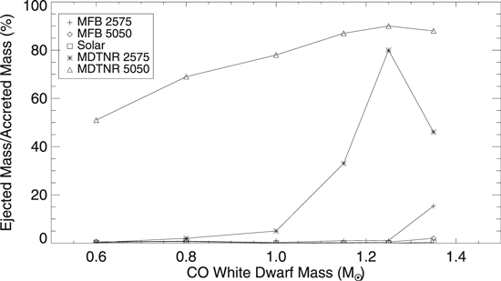
Figure 8. Ratio of ejected to accreted mass (in percent) as a function of CO WD mass. Neither the MFB nor the solar simulations eject much material and, thereby, the WD is growing in mass toward the Chandrasekhar limit. While the 25% WD–75% solar on the 1.25 M⊙ and 1.35 M⊙ simulations ejects 81% and 46% of the accreted mass, respectively, only 25% of the ejecta is WD material, and we predict that the WD is gaining in mass as a result of the CN outburst. The other sequences that eject a significant amount of material are the 50% WD and 50% MDTNR simulations on the massive WDs, but only half of the ejected gas is CO WD material.
Download figure:
Standard image High-resolution imageThose sequences with 50% WD matter and 50% solar matter MDTNR could have the WD either losing mass (MWD ≳ 1.0 M⊙) or gaining mass (MWD ≲ 1.0 M⊙), although only 50% of the material in the accreted layers is actual WD material. However, the peak luminosities, peak effective temperatures, and ejecta velocities do not agree with the observations. We assert, therefore, that for most observed CO CNe less than half of the material in the accreted region comes from the WD, and it is gaining in mass as a result of accretion, TNR, and ejection.
We end this subsection with plots of the evolution of the bolometric magnitude (Mbol) with time. Figure 9 shows the first hours of the evolution of both sets of simulations (top panel: 25_75 MDTNR; bottom panel: 50_50 MDTNR). Both panels show the rapid rise in Mbol as the energy produced in the nuclear burning region reaches the surface. Subsequently, they become roughly constant with time up to the end of the simulations. The Mbol value for the 1.35 M⊙ simulation with 25% WD and 75% solar material is lower than those of the other massive WDs, but they all appear to match observed CNe bolometric magnitudes. In contrast, Mbol for the 50% WD–50% solar MDTNR simulations all lie above those reported for typical CNe but may agree with the bright outliers seen in Kasliwal et al. (2011). For example, their Table 5 (Kasliwal et al. 2011) lists one nova in M82 with an absolute magnitude (Gunn-g) of −10.7 and one in M81 with an absolute magnitude of −9.9. Since these values refer to photometry obtained with the Gunn-g filter and our values are absolute bolometric magnitudes, we do not attempt to put them on the same sequence. In addition, we end our simulations before those novae would have been discovered. Our predicted absolute visual magnitudes rise slowly and reach values close to those plotted for peak Mbol after a few hours when the Teff has fallen below 104 K.
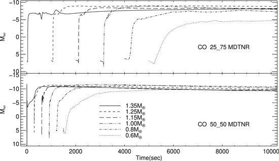
Figure 9. Top panel: variation with time of the absolute bolometric magnitude for the simulations where we used a composition of 25% WD matter and 75% solar after the TNR was well underway (MDTNR). After the initial few hundred seconds, they show a range in peak bolometric magnitude, but there is no correlation with CO WD mass. Bottom panel: the same plot as in the top panel but for a composition of 50% WD and 50% solar. The large amount of 12C in these simulations drives an initial shock in the most massive WD, and the other simulations all reach a peak Mbol around −10, which is extremely bright for the typical CN outburst. We, therefore, claim that this choice of composition does not agree with observations.
Download figure:
Standard image High-resolution image4.3. Detailed Look at a TNR
In this subsection, we describe the evolution of the 25% WD–75% solar MDTNR simulation on a 1.35M⊙ CO WD in detail. The gross properties of the evolution are found in Table 2. We accrete a solar mixture until the energy generation has reached a value of 1.3 × 10¹¹ erg gm−1 s−1, at which time the density is 9.0 × 10³ gm cm−3, the pressure is 8.8 × 10¹⁹ dynes cm−2, X = 0.71, the 12C abundance is 6.4 × 10⁻⁵ (by mass), and the temperature is 6.1 × 10⁷ erg gm−1 s−1. We then switch to the mixed composition and continue through the peak of the TNR and decline in temperature.
The switch in composition changes X to 0.53 and 12C to 0.13. As a result of the change in μ, the temperature jumps to 7.5 × 10⁷ K and the rate of energy generation to 4.1 × 10¹⁷ erg gm−1 s−1. It now takes 0.5 s for the energy generation to drop to 1.6 × 10¹⁴ erg gm−1 s−1 as the nuclear reactions move toward equilibrium. The convective region extends for 49 km, from the core–envelope interface (CEI: the mass zone where pure WD material connects to the accreted plus WD zones) toward the surface. Because the mass of the zones decreases with increasing radius, almost 96% of the accreted layers are in the convective region, so when convection reaches the surface (about 30 s later), there is no major change in the composition. At switchover, the mass fraction of 3He is 2.6 × 10⁻⁵, 2H is 2.1 × 10⁻⁵, and 7Be is zero. We report the evolution of 3He because it is converted to 7Be through the 3He(α,γ)7Be reaction. 7Be then decays to 7Li with a ∼53 day half-life.
After 41.4 s of evolution (times are given since the beginning of the switch in composition), the sequence reaches a temperature of 108 K just above the CEI, and after 50.4 s it reaches a second peak rate of energy generation of 3.4 × 10¹⁷ erg gm−1 s−1 at the CEI. The temperature in this mass zone is 2.5 × 10⁸ K, the density has fallen to 2.5 × 10³ gm cm−3, and convection has reached the surface layers of the WD. At 50.55 s the temperature has risen to 2.7 × 10⁸ K, and the density and nuclear energy generation have fallen to 2.0 × 10³ gm cm−3 and 1.8 × 10¹⁷ erg gm−1 s−1, respectively. At this time, the mass fractions of the positron-decaying nuclei in the nuclear burning region now exceed those of most of the stable CNO nuclei (13N = 1.7 × 10⁻², 14O = 1.3 × 10⁻¹, 15O = 2.6 × 10⁻³). Any further rise in energy generation will require these nuclei to decay before being able to capture another proton (Starrfield et al. 1972; Starrfield 1989). Meanwhile, the mass fraction of 3He has fallen to 7.6 × 10⁻⁶ and 2H to 4.8 × 10⁻⁹. The mass fraction of 7Be has risen to 1.3 × 10⁻⁵ at the CEI but is only 8.7 × 10⁻⁶ at the surface.
At an evolution time of 90.65 s (40 s after peak energy generation), the peak temperature of 3.41 × 10⁸ K is reached in the mass zones just above the CEI. The peak rate of energy generation in the same zone has declined to 3.3 × 10¹⁵ erg gm−1 s−1, and the density (in the same mass zone) to 6.0 × 10² gm cm−3. The temperatures throughout the nuclear burning region now exceed the Fermi temperature, lifting electron degeneracy, and the heating from the nuclear energy release throughout the envelope (the energy generation at the surface now exceeds 3 × 10¹⁴ erg gm−1 s−1) has driven the luminosity to 3.1 × 10⁴ L⊙ and Teff to its peak value of 106 K.
The outer layers are expanding at 20.8 km s−1 and the radius of the WD has increased to 3916 km from ∼2300 km. The expansion velocity at this time is far less than the escape velocity at this radius (∼104 km s−1). As the outer layers continue their expansion and begin to cool, convection begins to retreat from the outer layers, and thus the nuclear abundances in the material that will eventually be ejected are frozen in. The surface abundance of 3He is 4.4 × 10⁻⁶, that of 7Be is 1.7 × 10⁻⁵, and 7Li is 7.8 × 10⁻¹³. The destruction of the initial lithium in this type of evolution is well understood (Cameron & Fowler 1971) and implies that the 7Li and 7Be observed in nova ejecta (Izzo et al. 2015, 2018; Tajitsu et al. 2015, 2016; Molaro et al. 2016; Selvelli et al. 2018; Wagner et al. 2018; Woodward et al. 2020) must be coming from the decay of 7Be produced in the outburst.
We continue to evolve the simulation and, after 1.1 hr of expansion, the outer layers are becoming optically thin and their velocities have reached (because of radiation pressure) 1.4 × 10³ km s−1. The surface parameters are Teff = 1.3 × 10⁴ K and L = 1.3 × 10⁵ L⊙, and the outer radius is 5.2 × 1012 cm. At this radius, the escape speed has declined to <200 km s−1 so that ∼5 × 10⁻⁶M⊙ exceeds this speed, it is optically thin, and we tabulate it as ejected (see Table 2). The mass fraction of 7Be is 2.1 × 10⁻⁵ in the ejected gases.
5. Nucleosynthesis
In this section, we discuss the nucleosynthesis results from our simulations. We provide these results both as tables of the ejecta abundances in mass fraction and as production plots. Figure 11 (top panel: 1.0 M⊙ 25_75 MDTNR; bottom panel: 1.35 M⊙ 25_75 MDTNR) and Figure 12 (top panel: 1.0 M⊙ 50_50 MDTNR; bottom panel: 1.35 M⊙ 50_50 MDTNR) show the abundances of the stable isotopes (but also including 7Be) divided by the Lodders (2003) solar abundances. In these two figures, the x-axis is the atomic mass number, and the y-axis is the logarithmic ratio of the ejecta abundance divided by the solar abundance of the same isotope. The most abundant isotope of a given element is marked by an asterisk, and isotopes of the same element are connected by solid lines and labeled by the given element.
5.1. Production of 7Be in CO Classical Novae
Because of the recent discoveries of 7Be and its decay product 7Li in CNe ejecta, we report in this section that our mixed CO sequences are ejecting amounts of 7Be (which decays to 7Li after the simulation has ended) that are significantly enriched with respect to solar 7Li.
The amount of 7Li (actually produced as 7Be) in the ejected material in solar masses is shown in Figure 10 as a function of CO WD mass. All of our MDTNR sequences eject material enriched in 7Be, and the amount of enrichment is an increasing function of CO WD mass (Hernanz et al. 1996; José & Hernanz 1998). The nucleus produced during the TNR is 7Be. However, we do not follow the simulations sufficiently long for 7Be to decay to 7Li. All of the initial 7Li (or 6Li) in the accreting material is destroyed by the TNR. Both Tables 1 and 2 give the 7Li abundance (assuming that the 7Be has decayed) as the amount of 7Li ejected with respect to the solar value (N(7Li/H)ej/N(7Li/H)⊙).
Table 3. Comparison of Both 7Be Ejecta and Ejected Mass Results with José & Hernanz (1998) and Rukeya et al. (2017)
| CO WD Mass (M⊙): | 0.8 | 0.8 | 1.0 | 1.15 | 1.15 | 1.15a |
|---|---|---|---|---|---|---|
| Core %b | 25 | 50 | 50 | 25 | 50 | 50 |
| 7Be Ejecta Abundance by Mass | ||||||
| José & Hernanz (1998) | 4.4 × 10⁻⁷ | 9.6 × 10⁻⁷ | 3.1 × 10⁻⁶ | 6.0 × 10⁻⁶ | 8.1 × 10⁻⁶ | 3.1 × 10⁻⁶ |
| Rukeya et al. (2017) | 5.5 × 10⁻⁷ | 4.6 × 10⁻⁷ | 1.6 × 10⁻⁶ | 4.3 × 10⁻⁶ | 2.9 × 10⁻⁶ | |
| MFB (this work) | 8.2 × 10⁻⁷ | 7.0 × 10⁻⁷ | 1.4 × 10⁻⁶ | 5.9 × 10⁻⁶ | 4.4 × 10⁻⁶ | |
| MDTNR (this work) | 3.7 × 10⁻⁶ | 3.5 × 10⁻⁶ | 7.1 × 10⁻⁶ | 1.9 × 10⁻⁵ | 1.2 × 10⁻⁵ | |
| Ejected Mass (M⊙) | ||||||
| José & Hernanz (1998) | 7.0 × 10⁻⁵ | 6.4 × 10⁻⁵ | 2.3 × 10⁻⁵ | 1.5 × 10⁻⁵ | 1.3 × 10⁻⁵ | 6.3 × 10⁻⁶ |
| Rukeya et al. (2017) | 2.0 × 10⁻⁵ | 1.3 × 10⁻⁵ | 8.2 × 10⁻⁶ | 4.9 × 10⁻⁶ | 3.6 × 10⁻⁶ | |
| MFB (this work) | 3.7 × 10⁻⁷ | 4.1 × 10⁻⁷ | 4.4 × 10⁻⁸ | 9.8 × 10⁻⁸ | 1.3 × 10⁻⁷ | |
| MDTNR (this work) | 2.9 × 10⁻⁶ | 1.1 × 10⁻⁴ | 6.3 × 10⁻⁵ | 1.3 × 10⁻⁵ | 3.4 × 10⁻⁵ | |
Notes.
aThis sequence is reported in Table 2 of José & Hernanz (1998) and uses the updated opacities of Iglesias & Rogers (1993). bThe numbers in this row are the percent of core material in the simulation.Download table as: ASCIITypeset image
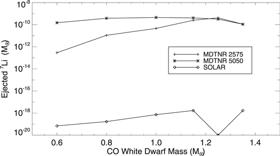
Figure 10. Predicted 7Li abundance in the ejecta as a function of WD mass in units of solar masses. The TNRs on CO WDs reach sufficiently high temperatures to deplete the initial 7Li present in the accreted material. The TNR then produces 7Be, which is mixed to the surface by strong convection during the TNR, and we actually plot that nucleus. 7Be decays (∼53 day half-life) after the end of the simulations. The simulations where we mix from the beginning (MFB) eject far less 7Li and are not plotted here. The simulation with solar abundances on a 1.25 M⊙ WD did not eject any material.
Download figure:
Standard image High-resolution imageIn Table 3 we compare the values in both our MFB and MDTNR studies with those in Hernanz et al. (1996), José & Hernanz (1998), and Rukeya et al. (2017). Rukeya et al. (2017) also provide a comparison with José & Hernanz (1998). Although there are differences between the microphysics in SHIVA (José & Hernanz 1998) and NOVA (opacities, equations of state, nuclear reaction rate library) and in the treatment of convection, except for the simulation at 0.6 M⊙, there is good agreement in our two predictions of 7Li ejecta abundances. The agreement is also good when comparing our results with Rukeya et al. (2017), who used MESA (Paxton et al. 2011, 2013, 2015, 2016, 2018) in their study.
The top row lists the WD mass, and the next row gives the specific mixture, either 25% WD matter or 50% WD matter. The next set of rows is the comparison of the 7Be results from each of the studies listed in the left column. The values in the first three rows all assume MFB. The results from José & Hernanz (1998) are higher than those of Rukeya et al. (2017) except for that of 25% WD matter at 0.8 M⊙. However, the last column, in which José & Hernanz (1998) redid the same evolutionary sequence, given in the previous column, but with the Iglesias & Rogers (1993) opacities, is nearly identical to that of Rukeya et al. (2017). Comparing our MFB simulations to those above, however, we find that our 7Be predictions exceed those of Rukeya et al. (2017) except for the simulation with 50% core matter on a 1.0 M⊙ WD. In contrast, they fall below those of José & Hernanz (1998) except for the simulations with 25% core matter at 0.8 M⊙ and their last simulation with the new opacities. Further, our MDTNR results are always larger than those reported in both of the other studies, and our MDTNR value for 50% core matter on a 1.15 M⊙ WD is 4 times larger than the value reported in José & Hernanz (1998) using newer opacities.
We also show in this table the comparison of the amount of ejected mass. For these cases, the sequences listed for José & Hernanz (1998) all eject more mass than either Rukeya et al. (2017) or our MFB set of calculations. Once José & Hernanz (1998) switch to an updated opacity table, however, their ejected mass drops by a factor of two and is more in line with Rukeya et al. (2017). Our MFB results are considerably smaller than either of the other two studies. In tests done to better understand this difference, we find that the introduction of new electron degenerate conductivities strongly affects the structure of the TNR and reduces the amount of ejected material. In addition, José & Hernanz (1998) use fewer mass zones (∼35) with (probably) larger masses. However, comparing our MDTNR values for the amount of mass ejected, we find they are larger than José & Hernanz (1998) for the three simulations with 50% core material but smaller for the 0.8 M⊙ (25% core matter) and the 1.15 M⊙ (25% core matter). Finally, except for the simulation with 25% WD matter at 0.8 M⊙, they are all larger than the equivalent simulations by Rukeya et al. (2017).
5.2. Enrichment of Other Nuclei in CO Nova Ejecta
Figures 11 and 12 show for both WD masses and compositions that 7Be, 15N, 17O, 31P, 35Cl, and 40Ca are significantly overproduced in CN ejecta. The results for the 1.0 M⊙ sequences are given in the top panels of Figures 11 and 12, and they show that both 7Be and 13C are about 300 times solar and 15N and 17O are nearly 104 times solar. In contrast, both 18O and 18F are depleted. None of the other isotopes are significantly enriched in the 1.0 M⊙ sequences. The 1.35 M⊙ results are shown in the bottom panels of Figures 11 and 12. Table 2 shows that peak temperatures in the 50% WD–50% solar sequences are much higher than in the 25% WD–75% solar sequences. Thus, 13C, 15N, 17O, 29S, 31P, and 35Cl are a great deal more enriched in the 50% WD–50% solar sequence. In addition, 7Be is enriched by about a factor of 300 and 22Ne is depleted, as is 23Na.
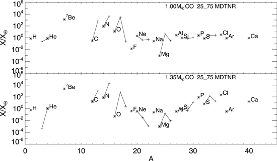
Figure 11. Top panel: abundances of the stable isotopes from hydrogen to calcium in the ejecta for the 1.0 M⊙ CO WD sequence. The x-axis is the atomic mass, and the y-axis is the logarithmic ratio of the abundance divided by the solar abundance (Lodders 2003). We also include 7Be in this plot, even though it is radioactive, because of its large overproduction. Both the initial 7Li and 6Li are depleted during the evolution. As in Timmes et al. (1995), the most abundant isotope of a given element is designated by an asterisk, and all isotopes of a given element are connected by solid lines. Any isotope above 1.0 is overproduced in the ejecta, and a number of light, odd isotopes are significantly enriched in the ejecta, as is 7Be. Bottom panel: the same plot as the top panel but for the 1.35 M⊙ simulation with 25% WD matter and 75% solar matter. Because of the higher peak temperature in this simulation, in addition to the light, odd isotopes of carbon, nitrogen, and oxygen, phosphorus and chlorine are also enriched.
Download figure:
Standard image High-resolution image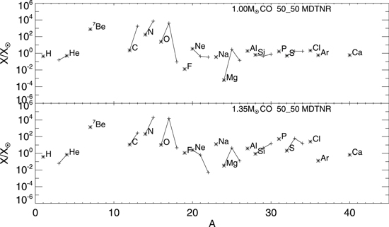
Figure 12. Top panel: the same plot as in Figure 11 but for the 1.0 M⊙ simulation with 50% WD matter and 50% solar matter. The most enriched species are 13C, 15N, 17O, and 7Be. Bottom panel: the same plot as the bottom panel in Figure 11 but for the simulation with a mass of 1.35 M⊙ and the 50% WD and 50% solar composition.
Download figure:
Standard image High-resolution imageTables 4–6 provide the detailed isotopic abundances in the ejected matter and allow us to compare the results for different WD masses. We do not include similar tables for the MFB simulations since they ejected hardly any material. Table 4 (no mixing of accreted with core material, hence, a solar mixture only) allows us to make predictions for those CNe or RNe that do not mix with WD matter. It shows that the ejected 12C abundance increases with WD mass, while 14N is relatively constant and the 16O abundance declines with increasing WD mass. The odd isotopes, such as 13C, increase with CO WD mass. For WD masses that exceed 1.0 M⊙, the 13C abundance always exceeds that of 12C. The 15N abundance increases with CO WD mass, and for some ranges in WD mass (1.0 M⊙ to 1.25 M⊙), its abundance exceeds that of 14N. In contrast, 18O, 26Al, and 27Al decrease with increasing CO WD mass. The abundance of 4He increases with WD mass, implying that more hydrogen is burned to helium to produce the energy produced in the outburst, since the amount of accreted mass declines with increasing WD mass.
Table 4. Ejecta or Surface Abundances for Solar Accretion and No Mixing with Core Materiala
| WD Mass (M⊙): | 0.6 | 0.8 | 1.0 | 1.15 | 1.25b | 1.35 |
|---|---|---|---|---|---|---|
| H | 7.0 × 10⁻¹ | 7.0 × 10⁻¹ | 7.0 × 10⁻¹ | 6.7 × 10⁻¹ | 6.7 × 10⁻¹ | 6.4 × 10⁻¹ |
| 3He | 7.5 × 10⁻¹² | 3.0 × 10⁻¹² | 2.0 × 10⁻⁷ | 2.0 × 10⁻⁸ | 5.6 × 10⁻¹³ | 8.6 × 10⁻¹¹ |
| 4He | 2.9 × 10⁻¹ | 3.0 × 10⁻¹ | 2.9 × 10⁻¹ | 3.1 × 10⁻¹ | 3.2 × 10⁻¹ | 3.5 × 10⁻¹ |
| 7Be | 1.0 × 10⁻¹³ | 1.4 × 10⁻¹³ | 1.5 × 10⁻¹⁰ | 4.5 × 10⁻¹¹ | 4.4 × 10⁻¹² | 5.7 × 10⁻¹¹ |
| 7Li | 0.0 | 0.0 | 6.3 × 10⁻¹¹ | 6.0 × 10⁻¹² | 0.0 | 7.4 × 10⁻¹⁵ |
| 12C | 1.9 × 10⁻⁴ | 3.4 × 10⁻⁴ | 4.6 × 10⁻⁴ | 8.8 × 10⁻⁴ | 7.2 × 10⁻⁴ | 1.1 × 10⁻³ |
| 13C | 1.1 × 10⁻⁴ | 3.0 × 10⁻⁴ | 6.0 × 10⁻⁴ | 1.5 × 10⁻³ | 1.1 × 10⁻³ | 2.1 × 10⁻³ |
| 14N | 7.5 × 10⁻³ | 7.8 × 10⁻³ | 3.3 × 10⁻³ | 3.4 × 10⁻³ | 3.3 × 10⁻³ | 3.8 × 10⁻³ |
| 15N | 5.9 × 10⁻⁶ | 4.2 × 10⁻⁵ | 4.8 × 10⁻³ | 3.6 × 10⁻³ | 4.4 × 10⁻³ | 2.3 × 10⁻³ |
| 16O | 1.9 × 10⁻³ | 1.1 × 10⁻³ | 4.6 × 10⁻⁴ | 3.0 × 10⁻⁵ | 7.2 × 10⁻⁶ | 1.7 × 10⁻⁵ |
| 17O | 1.2 × 10⁻⁵ | 7.7 × 10⁻⁶ | 1.2 × 10⁻⁴ | 9.4 × 10⁻⁶ | 9.6 × 10⁻⁷ | 6.1 × 10⁻⁷ |
| 18O | 5.7 × 10⁻⁹ | 3.1 × 10⁻⁹ | 1.3 × 10⁻⁷ | 1.8 × 10⁻⁸ | 3.2 × 10⁻¹⁰ | 8.1 × 10⁻¹⁰ |
| 18F | 4.6 × 10⁻¹¹ | 1.4 × 10⁻¹⁰ | 2.7 × 10⁻⁹ | 6.9 × 10⁻¹⁰ | 2.3 × 10⁻¹¹ | 5.6 × 10⁻¹¹ |
| 19F | 8.1 × 10⁻¹¹ | 1.3 × 10⁻¹¹ | 2.9 × 10⁻⁹ | 3.1 × 10⁻¹⁰ | 2.5 × 10⁻¹² | 6.3 × 10⁻¹¹ |
| 20Ne | 1.2 × 10⁻³ | 1.2 × 10⁻³ | 1.2 × 10⁻³ | 7.0 × 10⁻⁴ | 1.0 × 10⁻⁴ | 6.0 × 10⁻⁷ |
| 21Ne | 2.3 × 10⁻⁸ | 4.0 × 10⁻⁸ | 5.9 × 10⁻⁷ | 2.6 × 10⁻⁷ | 4.1 × 10⁻⁸ | 3.0 × 10⁻¹⁰ |
| 22Ne | 3.6 × 10⁻⁵ | 3.8 × 10⁻⁵ | 2.4 × 10⁻⁵ | 7.2 × 10⁻⁷ | 4.2 × 10⁻¹¹ | 1.6 × 10⁻⁹ |
| 22Na | 2.3 × 10⁻⁶ | 9.8 × 10⁻⁷ | 1.8 × 10⁻⁶ | 1.9 × 10⁻⁶ | 1.4 × 10⁻⁷ | 3.6 × 10⁻⁸ |
| 23Na | 6.3 × 10⁻⁶ | 3.2 × 10⁻⁶ | 5.3 × 10⁻⁶ | 5.7 × 10⁻⁶ | 3.9 × 10⁻⁷ | 1.1 × 10⁻⁷ |
| 24Mg | 5.6 × 10⁻⁸ | 3.2 × 10⁻⁸ | 3.4 × 10⁻⁶ | 3.7 × 10⁻⁷ | 4.4 × 10⁻⁹ | 2.8 × 10⁻⁹ |
| 25Mg | 6.0 × 10⁻⁴ | 3.3 × 10⁻⁴ | 5.6 × 10⁻⁵ | 6.3 × 10⁻⁶ | 3.9 × 10⁻⁷ | 3.7 × 10⁻⁸ |
| 26Mg | 7.7 × 10⁻⁵ | 2.4 × 10⁻⁵ | 5.3 × 10⁻⁶ | 4.3 × 10⁻⁷ | 1.6 × 10⁻⁸ | 2.4 × 10⁻⁹ |
| 26Al | 2.9 × 10⁻⁵ | 2.0 × 10⁻⁵ | 6.5 × 10⁻⁶ | 8.5 × 10⁻⁷ | 1.0 × 10⁻⁷ | 1.6 × 10⁻⁹ |
| 27Al | 9.7 × 10⁻⁵ | 1.4 × 10⁻⁴ | 3.0 × 10⁻⁵ | 4.3 × 10⁻⁶ | 4.3 × 10⁻⁷ | 1.9 × 10⁻⁸ |
| 28Si | 7.8 × 10⁻⁴ | 1.1 × 10⁻³ | 1.6 × 10⁻³ | 7.3 × 10⁻⁴ | 6.6 × 10⁻⁵ | 5.2 × 10⁻⁷ |
| 29Si | 4.0 × 10⁻⁵ | 3.6 × 10⁻⁵ | 2.2 × 10⁻⁵ | 1.3 × 10⁻⁵ | 9.1 × 10⁻⁷ | 6.0 × 10⁻⁸ |
| 30Si | 2.7 × 10⁻⁵ | 3.1 × 10⁻⁵ | 8.8 × 10⁻⁵ | 6.5 × 10⁻⁴ | 6.5 × 10⁻⁵ | 3.1 × 10⁻⁷ |
| 31P | 7.5 × 10⁻⁶ | 7.2 × 10⁻⁶ | 9.9 × 10⁻⁶ | 8.7 × 10⁻⁵ | 8.2 × 10⁻⁶ | 1.2 × 10⁻⁷ |
| 32S | 4.0 × 10⁻⁴ | 4.0 × 10⁻⁴ | 4.0 × 10⁻⁴ | 1.7 × 10⁻³ | 3.9 × 10⁻³ | 6.4 × 10⁻⁴ |
| 33S | 3.2 × 10⁻⁶ | 3.2 × 10⁻⁶ | 2.9 × 10⁻⁶ | 2.3 × 10⁻⁶ | 8.0 × 10⁻⁶ | 2.2 × 10⁻⁶ |
| 34S | 1.9 × 10⁻⁵ | 1.8 × 10⁻⁵ | 1.6 × 10⁻⁵ | 2.5 × 10⁻⁶ | 6.7 × 10⁻⁶ | 2.4 × 10⁻⁶ |
| 35Cl | 4.1 × 10⁻⁶ | 4.4 × 10⁻⁶ | 6.9 × 10⁻⁶ | 1.7 × 10⁻⁵ | 5.9 × 10⁻⁵ | 4.8 × 10⁻⁵ |
| 36Ar | 9.1 × 10⁻⁵ | 9.1 × 10⁻⁵ | 7.8 × 10⁻⁵ | 5.1 × 10⁻⁶ | 5.0 × 10⁻⁶ | 4.2 × 10⁻⁶ |
| 40Ca | 7.1 × 10⁻⁵ | 7.1 × 10⁻⁵ | 7.1 × 10⁻⁵ | 7.2 × 10⁻⁵ | 9.4 × 10⁻⁵ | 3.6 × 10⁻³ |
Notes.
aAll abundances are mass fraction. bThese are the surface zone abundances because no material was ejected.Download table as: ASCIITypeset image
Table 5. Ejecta Abundances for 25–75 MDTNR Mixture in CO White Dwarfsa
| WD Mass (M⊙) | 0.6 | 0.8 | 1.0 | 1.15 | 1.25 | 1.35 |
|---|---|---|---|---|---|---|
| H | 5.3 × 10⁻¹ | 5.2 × 10⁻¹ | 5.1 × 10⁻¹ | 4.8 × 10⁻¹ | 4.6 × 10⁻¹ | 4.3 × 10⁻¹ |
| 3He | 3.5 × 10⁻⁵ | 1.6 × 10⁻⁵ | 6.4 × 10⁻⁶ | 4.2 × 10⁻⁷ | 4.4 × 10⁻⁸ | 1.4 × 10⁻⁸ |
| 4He | 2.1 × 10⁻¹ | 2.1 × 10⁻¹ | 2.1 × 10⁻¹ | 2.3 × 10⁻¹ | 2.7 × 10⁻¹ | 3.1 × 10⁻¹ |
| 7Be | 6.0 × 10⁻⁷ | 3.7 × 10⁻⁶ | 1.2 × 10⁻⁵ | 1.9 × 10⁻⁵ | 2.0 × 10⁻⁵ | 2.1 × 10⁻⁵ |
| 7Li | 4.8 × 10⁻¹⁰ | 7.1 × 10⁻¹³ | 4.0 × 10⁻¹² | 4.4 × 10⁻¹³ | 3.1 × 10⁻¹³ | 4.6 × 10⁻¹³ |
| 12C | 9.0 × 10⁻² | 1.7 × 10⁻² | 9.3 × 10⁻⁴ | 1.0 × 10⁻² | 2.5 × 10⁻² | 5.0 × 10⁻² |
| 13C | 3.5 × 10⁻² | 8.2 × 10⁻² | 2.5 × 10⁻² | 1.2 × 10⁻² | 2.1 × 10⁻² | 3.8 × 10⁻² |
| 14N | 5.2 × 10⁻³ | 3.8 × 10⁻² | 1.0 × 10⁻¹ | 8.0 × 10⁻² | 7.9 × 10⁻² | 8.0 × 10⁻² |
| 15N | 2.2 × 10⁻⁵ | 2.1 × 10⁻³ | 2.1 × 10⁻² | 9.7 × 10⁻² | 1.2 × 10⁻¹ | 8.4 × 10⁻² |
| 16O | 1.3 × 10⁻¹ | 1.3 × 10⁻¹ | 1.2 × 10⁻¹ | 4.1 × 10⁻² | 1.4 × 10⁻³ | 5.4 × 10⁻⁴ |
| 17O | 2.4 × 10⁻⁴ | 2.0 × 10⁻³ | 1.3 × 10⁻² | 3.5 × 10⁻² | 1.6 × 10⁻² | 3.3 × 10⁻³ |
| 18O | 7.3 × 10⁻⁷ | 1.8 × 10⁻⁷ | 5.3 × 10⁻⁶ | 1.7 × 10⁻⁵ | 3.4 × 10⁻⁵ | 6.7 × 10⁻⁵ |
| 18F | 1.9 × 10⁻⁹ | 1.0 × 10⁻⁸ | 6.2 × 10⁻⁷ | 1.6 × 10⁻⁶ | 2.5 × 10⁻⁶ | 4.3 × 10⁻⁶ |
| 19F | 3.2 × 10⁻⁷ | 7.4 × 10⁻⁹ | 6.0 × 10⁻⁹ | 8.6 × 10⁻⁸ | 3.0 × 10⁻⁷ | 1.9 × 10⁻⁷ |
| 20Ne | 8.8 × 10⁻⁴ | 8.8 × 10⁻⁴ | 9.3 × 10⁻⁴ | 1.5 × 10⁻³ | 1.6 × 10⁻³ | 4.7 × 10⁻⁴ |
| 21Ne | 5.3 × 10⁻⁷ | 2.3 × 10⁻⁷ | 4.7 × 10⁻⁷ | 6.3 × 10⁻⁷ | 5.8 × 10⁻⁷ | 1.1 × 10⁻⁷ |
| 22Ne | 2.6 × 10⁻³ | 2.6 × 10⁻³ | 2.5 × 10⁻³ | 1.4 × 10⁻³ | 2.6 × 10⁻⁵ | 5.8 × 10⁻⁶ |
| 22Na | 1.8 × 10⁻⁶ | 8.6 × 10⁻⁷ | 1.4 × 10⁻⁶ | 2.3 × 10⁻⁶ | 5.3 × 10⁻⁶ | 4.4 × 10⁻⁶ |
| 23Na | 2.9 × 10⁻⁵ | 2.6 × 10⁻⁵ | 8.8 × 10⁻⁶ | 1.2 × 10⁻⁵ | 2.3 × 10⁻⁵ | 5.9 × 10⁻⁶ |
| 24Mg | 4.1 × 10⁻⁴ | 4.7 × 10⁻⁵ | 7.2 × 10⁻⁷ | 3.3 × 10⁻⁷ | 3.4 × 10⁻⁷ | 3.4 × 10⁻⁷ |
| 25Mg | 6.9 × 10⁻⁵ | 4.5 × 10⁻⁴ | 3.2 × 10⁻⁴ | 7.1 × 10⁻⁵ | 3.4 × 10⁻⁵ | 1.2 × 10⁻⁵ |
| 26Mg | 6.4 × 10⁻⁵ | 6.2 × 10⁻⁵ | 2.4 × 10⁻⁵ | 3.0 × 10⁻⁶ | 1.7 × 10⁻⁶ | 1.2 × 10⁻⁶ |
| 26Al | 1.6 × 10⁻⁸ | 3.2 × 10⁻⁶ | 8.4 × 10⁻⁵ | 2.2 × 10⁻⁵ | 8.5 × 10⁻⁶ | 2.4 × 10⁻⁶ |
| 27Al | 5.0 × 10⁻⁵ | 5.1 × 10⁻⁵ | 1.7 × 10⁻⁴ | 1.2 × 10⁻⁴ | 4.2 × 10⁻⁵ | 1.5 × 10⁻⁵ |
| 28Si | 5.7 × 10⁻⁴ | 5.7 × 10⁻⁴ | 6.3 × 10⁻⁴ | 1.6 × 10⁻³ | 9.1 × 10⁻⁴ | 4.8 × 10⁻⁴ |
| 29Si | 3.0 × 10⁻⁵ | 3.0 × 10⁻⁵ | 2.6 × 10⁻⁵ | 3.0 × 10⁻⁵ | 3.5 × 10⁻⁵ | 1.7 × 10⁻⁵ |
| 30Si | 2.0 × 10⁻⁵ | 2.0 × 10⁻⁵ | 2.5 × 10⁻⁵ | 1.3 × 10⁻⁴ | 5.2 × 10⁻⁴ | 2.3 × 10⁻⁴ |
| 31P | 5.7 × 10⁻⁶ | 5.7 × 10⁻⁶ | 5.7 × 10⁻⁶ | 2.4 × 10⁻⁵ | 2.9 × 10⁻⁴ | 1.5 × 10⁻⁴ |
| 32S | 3.0 × 10⁻⁴ | 3.0 × 10⁻⁴ | 3.0 × 10⁻⁴ | 3.0 × 10⁻⁴ | 2.2 × 10⁻³ | 2.7 × 10⁻³ |
| 33S | 2.4 × 10⁻⁶ | 2.4 × 10⁻⁶ | 2.4 × 10⁻⁶ | 2.2 × 10⁻⁶ | 1.7 × 10⁻⁵ | 1.6 × 10⁻⁴ |
| 34S | 1.4 × 10⁻⁵ | 1.4 × 10⁻⁵ | 1.4 × 10⁻⁵ | 1.1 × 10⁻⁵ | 7.7 × 10⁻⁶ | 1.2 × 10⁻⁴ |
| 35Cl | 3.0 × 10⁻⁶ | 3.0 × 10⁻⁶ | 3.2 × 10⁻⁶ | 5.9 × 10⁻⁶ | 1.4 × 10⁻⁵ | 2.7 × 10⁻⁴ |
| 36Ar | 6.8 × 10⁻⁵ | 6.8 × 10⁻⁵ | 6.8 × 10⁻⁵ | 4.7 × 10⁻⁵ | 3.0 × 10⁻⁶ | 3.2 × 10⁻⁵ |
| 40Ca | 5.4 × 10⁻⁵ | 5.4 × 10⁻⁵ | 5.4 × 10⁻⁵ | 5.4 × 10⁻⁵ | 5.4 × 10⁻⁵ | 1.0 × 10⁻³ |
Note.
aAll abundances are mass fraction.Download table as: ASCIITypeset image
Table 6. Ejecta Abundances for 50–50 MDTNR Mixture in CO White Dwarfsa
| WD Mass (M⊙): | 0.6 | 0.8 | 1.0 | 1.15 | 1.25 | 1.35 |
|---|---|---|---|---|---|---|
| H | 3.4 × 10⁻¹ | 3.3 × 10⁻¹ | 3.1 × 10⁻¹ | 3.0 × 10⁻¹ | 2.7 × 10⁻¹ | 2.2 × 10⁻¹ |
| 3He | 1.1 × 10⁻⁵ | 7.6 × 10⁻⁶ | 4.6 × 10⁻⁶ | 1.6 × 10⁻⁶ | 9.3 × 10⁻⁷ | 4.4 × 10⁻⁷ |
| 4He | 1.4 × 10⁻¹ | 1.4 × 10⁻¹ | 1.4 × 10⁻¹ | 1.6 × 10⁻¹ | 1.9 × 10⁻¹ | 2.4 × 10⁻¹ |
| 7Be | 9.3 × 10⁻⁷ | 3.5 × 10⁻⁶ | 7.1 × 10⁻⁶ | 1.2 × 10⁻⁵ | 1.4 × 10⁻⁵ | 1.6 × 10⁻⁵ |
| 7Li | 4.3 × 10⁻¹³ | 2.1 × 10⁻¹³ | 1.2 × 10⁻¹³ | 1.2 × 10⁻¹³ | 3.0 × 10⁻¹³ | 7.2 × 10⁻¹⁴ |
| 12C | 1.0 × 10⁻¹ | 2.3 × 10⁻² | 6.8 × 10⁻³ | 1.7 × 10⁻² | 2.5 × 10⁻² | 6.8 × 10⁻² |
| 13C | 1.3 × 10⁻¹ | 1.5 × 10⁻¹ | 6.8 × 10⁻² | 1.2 × 10⁻² | 2.0× 10⁻² | 3.6 × 10⁻² |
| 14N | 3.0 × 10⁻² | 9.6 × 10⁻² | 1.9 × 10⁻¹ | 2.0 × 10⁻¹ | 1.9 × 10⁻¹ | 1.7 × 10⁻¹ |
| 15N | 2.2 × 10⁻⁴ | 5.3 × 10⁻³ | 3.2 × 10⁻² | 8.8 × 10⁻² | 1.7 × 10⁻¹ | 2.0 × 10⁻¹ |
| 16O | 2.5 × 10⁻¹ | 2.4 × 10⁻¹ | 2.3 × 10⁻¹ | 1.8 × 10⁻¹ | 4.9 × 10⁻² | 1.9 × 10⁻² |
| 17O | 1.4 × 10⁻³ | 4.9 × 10⁻³ | 1.6 × 10⁻² | 4.3 × 10⁻² | 8.6 × 10⁻² | 3.2 × 10⁻² |
| 18O | 3.9 × 10⁻⁷ | 8.2 × 10⁻⁷ | 2.0 × 10⁻⁶ | 8.3 × 10⁻⁶ | 3.0 × 10⁻⁵ | 6.0 × 10⁻⁶ |
| 18F | 2.1 × 10⁻⁸ | 4.3 × 10⁻⁸ | 5.0 × 10⁻⁷ | 4.0 × 10⁻⁶ | 9.4 × 10⁻⁶ | 1.9 × 10⁻⁶ |
| 19F | 2.6 × 10⁻⁸ | 8.6 × 10⁻¹⁰ | 5.2 × 10⁻⁹ | 4.2 × 10⁻⁸ | 7.3 × 10⁻⁷ | 1.0 × 10⁻⁶ |
| 20Ne | 5.8 × 10⁻⁴ | 6.0 × 10⁻⁴ | 6.7 × 10⁻⁴ | 1.1 × 10⁻³ | 2.6 × 10⁻³ | 1.3 × 10⁻³ |
| 21Ne | 3.2 × 10⁻⁸ | 1.1 × 10⁻⁷ | 2.2 × 10⁻⁷ | 3.8 × 10⁻⁷ | 1.1 × 10⁻⁶ | 4.0 × 10⁻⁷ |
| 22Ne | 5.0 × 10⁻³ | 5.0 × 10⁻³ | 4.9 × 10⁻³ | 4.0 × 10⁻³ | 4.2 × 10⁻⁴ | 1.9 × 10⁻⁴ |
| 22Na | 1.2 × 10⁻⁶ | 2.9 × 10⁻⁷ | 4.1 × 10⁻⁷ | 1.1 × 10⁻⁶ | 5.1 × 10⁻⁶ | 1.2 × 10⁻⁶ |
| 23Na | 2.2 × 10⁻⁵ | 2.1 × 10⁻⁵ | 1.3 × 10⁻⁵ | 1.3 × 10⁻⁵ | 4.1 × 10⁻⁵ | 2.2 × 10⁻⁵ |
| 24Mg | 1.3 × 10⁻⁴ | 1.1 × 10⁻⁶ | 6.4 × 10⁻⁷ | 7.1 × 10⁻⁷ | 1.4 × 10⁻⁶ | 2.4 × 10⁻⁶ |
| 25Mg | 2.0 × 10⁻⁴ | 3.2 × 10⁻⁴ | 2.4 × 10⁻⁴ | 1.8 × 10⁻⁴ | 2.3 × 10⁻⁴ | 8.4 × 10⁻⁵ |
| 26Mg | 4.2 × 10⁻⁵ | 3.7 × 10⁻⁵ | 1.2 × 10⁻⁵ | 9.1 × 10⁻⁶ | 2.0 × 10⁻⁵ | 6.8 × 10⁻⁶ |
| 26Al | 1.8 × 10⁻⁷ | 1.2 × 10⁻⁵ | 6.6 × 10⁻⁵ | 7.7 × 10⁻⁵ | 2.9 × 10⁻⁵ | 2.8 × 10⁻⁵ |
| 27Al | 3.3 × 10⁻⁵ | 3.9 × 10⁻⁵ | 1.2 × 10⁻⁴ | 3.0 × 10⁻⁴ | 1.4 × 10⁻⁴ | 1.3 × 10⁻⁴ |
| 28Si | 3.8 × 10⁻⁴ | 3.8 × 10⁻⁴ | 4.2 × 10⁻⁴ | 7.7 × 10⁻⁴ | 2.1 × 10⁻³ | 9.9 × 10⁻⁴ |
| 29Si | 2.0 × 10⁻⁵ | 2.0 × 10⁻⁵ | 1.6 × 10⁻⁵ | 1.3 × 10⁻⁵ | 9.2 × 10⁻⁵ | 3.3 × 10⁻⁵ |
| 30Si | 1.4 × 10⁻⁵ | 1.4 × 10⁻⁵ | 1.8 × 10⁻⁵ | 4.0 × 10⁻⁵ | 7.9 × 10⁻⁴ | 4.6 × 10⁻⁴ |
| 31P | 3.8 × 10⁻⁶ | 3.8 × 10⁻⁶ | 3.8 × 10⁻⁶ | 5.5 × 10⁻⁶ | 3.0 × 10⁻⁴ | 2.9 × 10⁻⁴ |
| 32S | 2.0 × 10⁻⁴ | 2.0 × 10⁻⁴ | 2.0 × 10⁻⁴ | 2.0 × 10⁻⁴ | 4.9 × 10⁻⁴ | 3.4 × 10⁻³ |
| 33S | 1.6 × 10⁻⁶ | 1.6 × 10⁻⁶ | 1.6 × 10⁻⁶ | 1.6 × 10⁻⁶ | 4.0 × 10⁻⁶ | 2.4 × 10⁻⁴ |
| 34S | 9.3 × 10⁻⁶ | 9.3 × 10⁻⁶ | 9.2 × 10⁻⁶ | 8.7 × 10⁻⁶ | 4.4 × 10⁻⁶ | 1.4 × 10⁻⁴ |
| 35Cl | 2.0 × 10⁻⁶ | 2.0 × 10⁻⁶ | 2.1 × 10⁻⁶ | 2.7 × 10⁻⁶ | 6.8 × 10⁻⁶ | 2.5 × 10⁻⁴ |
| 36Ar | 4.6 × 10⁻⁵ | 4.6 × 10⁻⁵ | 4.5 × 10⁻⁵ | 4.0 × 10⁻⁵ | 1.1 × 10⁻⁵ | 4.8 × 10⁻⁵ |
| 40Ca | 3.6 × 10⁻⁵ | 3.6 × 10⁻⁵ | 3.6 × 10⁻⁵ | 3.6 × 10⁻⁵ | 3.6 × 10⁻⁵ | 5.9 × 10⁻⁵ |
Note.
aAll abundances are mass fraction.Download table as: ASCIITypeset image
Table 5 gives the ejecta abundances for the mixture with 25% WD matter and 75% solar matter. The abundance of 7Be increases with increasing WD mass, and the initial 7Li is destroyed by the TNR. Both 12C and 13C are produced in the higher mass CO WDs, but there is more 12C than 13C produced for most WD masses. The abundance of 14N is roughly constant for the more massive CO WDs, while 15N reaches a peak abundance of 0.12 for a 1.25 M⊙ WD and is nearly that value for the other massive WDs. Moreover, its abundance exceeds that of 14N for WD masses from 1.15 M⊙ to 1.35 M⊙. In contrast to the solar abundance results (Table 4), the abundances of 17O, 18O, and 31P increase with WD mass. 26Al and 27Al reach a maximum abundance at 1.0M⊙ and then decline with increasing WD mass as the peak temperature in the nuclear burning region increases during the TNR. The ratio of their abundances is ∼0.2.
Table 6 provides a listing of the ejecta abundances for the mixture with 50% WD matter and 50% solar matter. Again, the ejected hydrogen abundance declines with increasing WD mass because the total envelope mass decreases with increasing WD mass, so it takes more hydrogen burning to provide the energy observed in the outburst. The 7Be abundance reaches a maximum at 1.25 M⊙, but the 7Li abundance decreases with increasing WD mass. 7Li is essentially destroyed in the outburst, so, again, all of the 7Li observed in CNe ejecta must be coming from the decay of 7Be produced in the outburst.
The ejecta abundance of 12C increases with WD mass, while that of 13C is maximum at 0.8 M⊙ and then declines. The abundance of 14N increases with WD mass, while 15N increases and reaches a maximum at 1.25 M⊙. In fact, the odd isotopes are so abundant that molecular studies of CN ejecta should discover large amounts of 12C15N, 13C14N, and in some cases 13C15N. The detection of these molecular species would provide strong observational support for the results of these simulations and possibly could be used to determine the composition of the underlying WD.
The abundance of 16O declines with increasing WD mass, while that of 17O increases but reaches a maximum value at 1.25 M⊙. In contrast, that of 18O increases as the WD mass increases. The abundance of 26Al reaches a maximum at 1.0 M⊙, while that of 27Al increases up to 1.35 M⊙. The ratio of their abundances varies from about 0.3 down to about 0.1, values that are smaller than found in the 25% WD–75% solar MDTNR studies. The abundances of 22Na, 31P, and 35Cl also increase with CO WD mass.
6. CNe and CVs Are Likely One Channel of SN Ia Progenitors
The progenitors of SN Ia explosions are as yet unknown, although SN Ia are of great importance to both galactic chemical evolution and as probes of the evolution of the universe. Originally, the SD scenario, with the WD accreting from the secondary and growing in mass toward the Chandrasekhar limit, was preferred, but this scenario is now disfavored by many (Gilfanov & Bogdán 2010, and references therein). The other scenario, the DD scenario, which involves either a merger or collision between two CO WDs, is now thought to be the major channel for SN Ia explosions. The cause of this switch in the preferred explosion paradigm is a number of perceived problems with the SD scenario that need to be addressed. In this section, we discuss four of those problems and show that they are, in fact, not problems at all.
The first major problem, which is relevant to the simulations presented in the earlier sections, is the common assumption, based on the analyses of the ejecta abundances and ejecta masses of CNe outbursts, that the WD is decreasing in mass as a consequence of the TNR and resulting explosion. We have now shown in earlier sections, however, that assumption is incorrect and, in fact, the WD in a CO nova outburst is gaining in mass.
We have also shown in previous studies that the WD is growing in mass when there is no mixing of the accreting material with WD core matter as may be occurring in CVs in general (Starrfield 2014, 2017, and references therein). These latter results are based on studies with both NOVA and MESA and imply that the consequence of mass transfer in CVs is the increasing mass of the WD. Moreover, the calculations of Hillman et al. (2016) show that high mass accretion rates also result in the WDs growing in mass. One concern, nevertheless, is that the large number of CVs in the galaxy may result in too many SN Ia explosions. It is the mass of the secondary, however, that also determines the ultimate fate of the system. It is possible, for example, that in many CV systems the secondary has too little mass and, therefore, mass transfer ends before the WD has reached the Chandrasekhar limit.
The second perceived problem is due to the interpretation of the calculations of Nomoto (1982) and Fujimoto (1982a, 1982b). A reproduction of their results can be found as Figure 5 in Kahabka & van den Heuvel (1997). The figure shows that the space describing the consequences of mass accretion rate as a function of the mass of the accreting WD can be divided into three regions. For the lowest mass accretion rates, at all WD masses, it is predicted that accretion results in hydrogen flashes that resemble those of CNe and, as already discussed, the WD is thought to be losing mass. However, the purpose of this paper has been to provide a broad range of simulations at low  that show a WD accreting at low rates is gaining in mass. Hillman et al. (2016) have investigated the consequences of accretion at higher rates and also find that the WD is growing in mass. Thus, mass-accreting systems with a broad range in WD mass and
  must be included in the classes of SN Ia progenitors.
A third problem relates to the upper region on the Nomoto (1982) and Fujimoto (1982a, 1982b) plots, which shows the results for the highest accretion rates and predicts for all WD masses that the radius of the WD will grow rapidly to red giant dimensions, accretion will be halted, and any further evolution will await the collapse of the extended layers. These systems, therefore, cannot be SN Ia progenitors. However, we have done extensive studies of solar accretion onto WDs using both NOVA and MESA, and our version of their diagram can be found in Starrfield (2014, 2017). Our fully hydrodynamic studies show, for the highest mass accretion rates on the most massive WDs, steady hydrogen burning (see below) is occurring, followed by recurring helium flashes. The helium flashes do not result in ejection, and the WDs are again growing in mass. Hillman et al. (2016) also report that helium flashes do not eject material.
The fourth problem is based on the existence of the intermediate regime identified by Nomoto (1982) and Fujimoto (1982a, 1982b), where the material is predicted to burn steadily at the rate it is accreted. The central  of this region is nominally ∼3 × 10⁻⁷M⊙ yr−1, and it does have a slight variation with WD mass. Those systems that are accreting at the steady nuclear burning rate are supposedly evolving horizontally in this plot toward higher WD mass, and, by some unknown mechanism, the mass transfer in the binary system is stuck in this mass accretion range. van den Heuvel et al. (1992) predicted that it was only the systems in this region that were SN Ia progenitors via the SD scenario. They identified the supersoft X-ray sources (SSS) as those systems, based on their luminosities and effective temperatures. The SSS are luminous, massive WDs discovered by ROSAT (Trümper et al. 1991). They are binaries, with luminosities L* ∼ 1037–38 erg s−1 and effective temperatures in the range (3–7) × 105 K (Branch et al. 1995; Kahabka & van den Heuvel 1997; Cowley et al. 1998).
However, in more recent studies of accretion without mixing, an expanded study of the stability of thin shells can be found in Yoon et al. (2004, and references therein), who investigated the accretion of helium-rich and hydrogen-rich material onto WDs. Using their results, we find that sequences in the steady nuclear burning regime begin in their stable region, but with continued accretion they evolve into instability. In addition, their study shows that the evolutionary sequences at these  exhibit the Schwarzschild & Härm (1965) thin shell instability, which implies that steady burning does not occur. We identify these systems, therefore, with those CVs (dwarf, recurrent, symbiotic novae) that show no core material either on the surface of the WD or in their ejecta.
Given that the SSS were the only systems that were predicted to be SD Ia progenitors, it was expected that they would be detected by consequence of the long periods of luminous X-ray and UV emission on the surrounding interstellar medium (ISM). In addition, this extreme emission should still be evident in the ISM surrounding recent SN Ia explosions. As an example, we quote from Graur & Woods (2019): “For the WD to efficiently grow in mass, the accreted hydrogen must undergo stable nuclear burning on its surface. This means the progenitor system will be a luminous source of soft X-ray emission (a supersoft X-ray source, SSS, van den Heuvel et al. 1992) for at least some period of time before the explosion.” Similar statements can also be found in Gilfanov & Bogdán (2010) and Kuuttila et al. (2019). Such emission has not been found, and the absence of evidence has been used to eliminate the SD scenario even in the most recent studies. However, observations of CNe and CVs, which we now identify as possible SN Ia progenitors, show that they do not spend a large amount of time at high luminosities and effective temperatures.
Moreover, some RNe are repeating sufficiently often that their WDs must have grown in mass such that they are now close to the Chandrasekhar limit. One such system is the “rapidly recurring” RN in M31 (M31N 2008-12a), which is outbursting about once per year and has opened a large cavity in the ISM surrounding the system (Henze et al. 2015, 2018; Darnley et al. 2016, 2017a, 2017b, 2019). It is neither X-ray nor UV luminous between outbursts.
7. Discussion
Fortunately for this study, the recent multi-D studies of convection in the accreted layers of WDs (Casanova et al. 2010, 2011a, 2011b, 2016, 2018; José 2014; José et al. 2020, and references therein) implied that we could reasonably approximate their results by accreting a hydrogen-rich (solar abundance) layer and then switching to a mixed composition once the TNR was underway and convection had begun. A similar technique was used by José et al. (2007), who explored a variety of timescales for mixing the WD material into the accreted layers, once convection was underway, and found that using short timescales was warranted. Their work has now been updated by José et al. (2020), who combined 1D evolution with multi-D evolution and found sufficient mixing of the core with the envelope to agree with the observations.
Therefore, we have used NOVA to study the consequences of TNRs on WDs of various masses using three different compositions. In all cases we find that more mass is accreted than ejected and, therefore, the WD is growing in mass. We have used two different techniques to treat the accreting material. In the first we assumed that the solar material is mixed from the beginning of accretion (MFB). This is the technique used both by us and others in the past because there was no agreement on when and how WD material was mixed up into the accreting matter. Neither the consequences of our solar mixture accretion simulations nor those where we mix from the beginning of accretion (MFB; Tables 1 and 2) agree with the observations of CNe outbursts with respect to ejecta masses and velocities.
Switching to a mixed composition once the TNR is ongoing and a major fraction of the accreted material is convective, however, provides a range of model outcomes that are more compatible with observed CNe physical parameters reported in the literature. The simulations with 25% CO WD matter and 75% solar matter (MDTNR) appear to fit the observations better than those with 50% CO WD matter and 50% solar matter (MDTNR). Nevertheless, NOVA is able to only follow one outburst, and reaching close to the Chandrasekhar limit requires many such cycles of accretion–TNR–ejection–accretion. While this has yet to be done with either CO- or ONe-enriched material (this may have been done in the study of Rukeya et al. 2017, but they only reported their ejected mass, not the accreted mass), multicycle evolution and growth in mass of the WD have been done with solar accretion studies (Starrfield 2014; Hillman et al. 2016; Starrfield 2017). We note that the multicycle studies reported in Starrfield (2014, 2017) were done with MESA (Paxton et al. 2011, 2013, 2018, and references therein), while those described by Hillman et al. (2016) were done with the code of Kovetz et al. (2009, and references therein). Given these studies with multiple codes, therefore, we feel that the consequence of the CN outburst is the growth in mass of the WD under all situations. Therefore, we extended our simulations to WD masses of 1.35 M⊙.
Of great importance, some of the ejected isotope abundances in the simulations also fit the isotopic ratios measured for some presolar grains, suggesting that these grains come from CNe ejecta (Bose & Starrfield 2019). Bose & Starrfield (2019) compared the compositions of 30 presolar SiC grains with the ejected isotopic abundances in Tables 5 and 6. The simulations with 25% WD matter and 75% solar matter with CO WD masses from 0.8 M⊙ to 1.35 M⊙ provide the best fits to the measured isotopic data in four SiC grains. In addition, one grain matches the 50% WD and 50% solar 1.35 M⊙ MDTNR simulation. To the best of our knowledge, this is the first study that successfully applies CO nova simulations to both observations of nova dust and presolar grains of nova origin. Previous studies that attempted to understand SiC nova grain candidates used ONe nova simulations from José & Hernanz (1998), which mandated mixing >95% of solar matter with <5% of CN ejected matter to account for the grains’ compositions (Amari et al. 2001). Such mixing is not required for other grain types (e.g., SiC X grains from supernovae). The other assumption, that the binary companion to the WD had to be a main-sequence star, made the assignment of nova candidate grains as bona fide nova grains even more uncertain. However, using the simulations described here, we require less than 25% of solar system material be mixed with the CO nova ejecta to account for the grain compositions (Bose & Starrfield 2019).
These simulations show that for CO WD mass ≥1.15 M⊙ the mass fraction of 7Li (7Be) ejected is either 2 × 10⁻⁵ (25% WD matter and 75% solar matter: Table 5) or 10−5 (50% WD matter plus 50% solar matter: Table 6). The amount of ejected mass for the same WD range is ∼10−5M⊙ for the 25% WD matter and 75% solar matter simulations and ∼2 × 10⁻⁵ for the 50% WD matter plus 50% solar matter simulations, as given in Table 2. Interestingly, their product implies an ejected 7Li mass of ∼2 × 10⁻¹⁰ M⊙ for either composition. If we take a value for the CN rate of 50 yr−1 (Shafter 2017), a lifetime for the galaxy of 1010 yr, and our production values, we arrive at a predicted abundance of ∼100M⊙ for the 7Li produced by CNe in the galaxy.
These results confirm that CO novae are overproducing 7Be, which decays to 7Li. The amount of 7Be we predict from our simulations, in combination with the observations, allows us to assert that CNe are responsible for a significant fraction of the 7Li in the galaxy. Moreover, the observations of 7Be and 7Li found in the early high-dispersion optical spectra of the ejected material from CN outbursts (both CO and ONe; Izzo et al. 2015, 2018; Tajitsu et al. 2015, 2016; Molaro et al. 2016; Selvelli et al. 2018; Wagner et al. 2018; Woodward et al. 2020) report much higher values than we predict, in fact, at least 10 times higher than previously predicted (Starrfield et al. 1978; Hernanz et al. 1996; José & Hernanz 1998).
We also address the question: what is the total amount of7Li in the galaxy? The number usually quoted is ∼150 M⊙ (Hernanz et al. 1996; Molaro et al. 2016). However, we arrive at a different value. Lodders et al. (2009) give a value of 2.0 × 10⁻⁹ for the solar system meteoritic abundance of 7Li/H by number. We convert to mass fraction by multiplying by 7 and obtain 1.4 × 10−8 for X(7Li)/X(H). We assume that the total mass of the galaxy is ∼1011 M⊙ and the mass fraction of hydrogen is 0.71 (Lodders & Palme 2009; Lodders et al. 2009). Therefore, the total mass of 7Li in the galaxy should be 0.71 × 1011 × 1.4 × 10−8 or ∼1000 M⊙. The most recent discussion of the importance of CNe for 7Li in the galaxy is that of Cescutti & Molaro (2019, and references therein), who address the discoveries of 7Li and 7Be in CN ejecta. Finally, the primordial 7Li abundance in the galaxy is ∼80 M⊙, requiring a galactic source of 7Li (Fields 2011). 6Li is produced by spallation and not by nuclear reactions in stars, however, so there should not be a correlation in the abundances of these two isotopes in stellar sources.
Our technique, of first accreting a solar mixture and then switching to a mixed composition, can be compared to calculations where a mixed composition was used from the beginning of the simulation (Hernanz et al. 1996; José & Hernanz 1998; Rukeya et al. 2017). They accreted onto both CO and ONe WDs in order to determine the 7Li production from CNe but did not study CO WDs as massive as in this work. They assumed two mixed compositions from the beginning (either 25% WD material or 50% WD material) with a solar (Lodders & Palme 2009) 3He abundance of 8.46 × 10⁻⁵. All our simulations used a 3He mass fraction (Lodders 2003) of 3.41 × 10⁻⁵. Since the production of 7Be occurs through the 3He(α,γ)7Be reaction, a higher abundance of 3He is expected to result in a higher 7Be abundance (Hernanz et al. 1996; José & Hernanz 1998). However, the larger accreted mass in our simulations resulted both in a higher peak temperature and also stronger convection (transporting the 7Be more rapidly to the surface layers). These effects combined resulted in a larger amount of 7Be than reported in either Hernanz et al. (1996), José & Hernanz (1998), or Rukeya et al. (2017).
Rukeya et al. (2017) also compared their simulations to the total observed amount of 7Li in the galaxy (∼150 M⊙ given in Hernanz et al. 1996). They argued that CO novae are producing about 10% of galactic lithium. Our simulations, however, produce at least 1.5 times more 7Li than their simulations (or those of José & Hernanz 1998). In addition, we have also followed the 7Li production on more massive WDs, achieving about a factor of two enrichment over their results. Therefore, it seems likely that CO novae can produce a significant amount of stellar 7Li. In Tables 1 and 2 we give the ejected 7Li abundance in the same units as in Hernanz et al. (1996) so that a direct comparison can be made.
We find that the amount of accreted material is an inverse function of the initial abundance of 12C. Accreting solar material (rather than mixed) allows for more matter to be accreted. Reducing the metallicity to values seen in the LMC, SMC, or even lower also reduces the initial 12C, allowing more material to be accreted before the TNR is initiated (Starrfield et al. 1999; José et al. 2007) and the accreted material mixes with WD matter. Finally, either no mixing with the WD (RNe) or mixing too early with the CO WD (MFB) results in an outburst that ejects less material than is accreted, and the WD is also growing in mass.
Finally, there is little to no observational evidence for mixing of accreted matter with WD matter in RN explosions. While all CNe are thought to be recurrent, by convention RNe are those novae that have experienced multiple recorded outbursts in the last 150 yr or so. Pure solar accretion studies show that virtually no material is ejected and, therefore, those WDs must be growing rapidly in mass (Starrfield et al. 2012a; Starrfield 2014). In addition, mixing may occur in these CNe, but since the outer layers of the WD consist of material that has undergone previous CN outbursts, and the outburst has left a helium-enriched layer behind, it will be helium-enriched material that is mixed into the accreted layers in addition to 12C-enriched material. In fact, spectroscopic studies of CNe and RNe ejecta show that this material is strongly enriched in helium and to amounts that suggest that helium has been mixed up from below and is not just the residue of the hot-hydrogen burning reactions that drove the TNR.
8. Conclusions
- 1.The amount of accreted material is an inverse function of the initial abundance of 12C.
- 2.By first accreting solar material (rather than mixed), more matter is accreted than if we assumed mixing from the beginning. Reducing the metallicity to values in agreement with the Magellanic Clouds, or even lower, further reduces the initial 12C abundance, allowing more material to be accreted before the TNR is initiated (Starrfield et al. 1999; José et al. 2007).
- 3.Either no mixing with the WD (solar accretion) or mixing too early with the WD (MFB) results in an outburst that is less violent, and little material (accreted plus WD) is ejected during the outburst. This also causes the CO WD to grow in mass. We have shown this by following one outburst with NOVA and repeated outbursts with MESA (Starrfield et al. 2016).
- 4.Multidimensional studies show that there is sufficient mixing during the TNR to agree with observations of the ejecta abundances (Casanova et al. 2018; José et al. 2020, and references therein). This mixing occurs via convective entrainment (dredge-up of WD outer layers into the accreted material) during the TNR and does not affect the total amount of accreted material since it occurs after the accretion phase of the outburst.
- 5.Simulations with 25% CO WD and 75% solar matter, mixed after the TNR is underway, eject only a fraction of the accreted material. Therefore, the WD is growing in mass as a result of the classical nova phenomena (see Figure 8).
- 6.Simulations with 50% CO WD and 50% solar matter, mixed after the TNR is underway, ejected a larger fraction of accreted material but not as much as was accreted. Therefore, these simulations, with more 12C, also imply that the WD is growing in mass as a result of the classical nova phenomena. They also reached higher peak temperatures and ejected more material, moving at higher velocities than those with only 25% WD and 75% solar matter.
- 7.Our simulations confirm that CO novae are overproducing 7Be, which decays to 7Li after we have ended our simulations. This result is in agreement with the observations of enriched 7Be in CN explosions, although the observed values exceed our predictions and those of others.
- 8.
- 9.While we do not rule out the SSS as SN Ia progenitors, their observed numbers suggest that they are likely to be an extremely small channel, with typical CVs being a major channel. Finally, the observations of SN Ia explosions alone suggest that there are multiple channels for their progenitors (Polin et al. 2019, and references therein).
- 10.Our results indicate that even systems with low accretion rates,
 < 10−9 M⊙ yr−1, can produce CNe in which the WD is growing in mass toward the Chandrasekhar limit. In combination with the results of Hillman et al. (2015, 2016, done with a different code and higher mass accretion rates), our simulations add a considerable area to the –WD mass plane, where evolution to a SN Ia is possible. It is no longer necessary to assume that the only area in which the WD grows in mass is that region designated as the “steady burning” region.


We acknowledge useful discussion and encouragement from M. Darnley, E. Aydi, J. José M. Hernanz, A. Heger, S. Kafka, L. Izzo, P. Molaro, M. della Valle, A. Shafter, and the attendees at EWASS18, COSPAR 2018, and HEAD 2019 for their comments. We thank J. José and A. Shafter for their comments on an earlier draft that greatly improved this manuscript. This work was supported in part by NASA under the Astrophysics Theory Program grant 14-ATP14-0007 and the U.S. DOE under Contract Nos. DE-FG02-97ER41041 and DE-AC05-00OR22725. S.S. acknowledges partial support from NASA, NSF, and HST grants to ASU, W.R.H. is supported by the U.S. Department of Energy, Office of Nuclear Physics, and C.E.W. acknowledges support from NASA grant 80NSSC19K0868 and NSF.
Appendix: Checking Convergence and Composition Change
In order to check both the convergence and the effects of switching the composition on our CN simulations, in this appendix we report on additional simulations for a CO WD mass of 1.35 M⊙. For this WD mass, we have computed three additional initial models with 95, 200, or 300 mass zones and used them to follow the evolution through the TNR and return to quiescence. With these three models, plus the original one with 150 mass zones, we tested the effects of switching the composition by switching at two different times in the evolution prior to the steep rise to peak temperature.
The results from the new simulations are given in Tables A1 and A2. Table A1 gives the initial conditions and evolutionary results, while Table A2 gives the temperature, density, chemical composition, and energy generation in the zone with peak energy generation both before and after the switch. The number of mass zones in the simulation is the first row in the table. There are two columns for each choice of mass zoning because we evolved two sequences for each mass zone. Our test of the effects of composition switching was to stop the solar accretion simulation at two different times in the rise to the peak of the TNR and then switch to the new composition. Those two times were either 107 or 1011 erg gm−1 s−1, and the latter value is what we used in the simulations in the earlier sections.
Table A1. Initial and Evolutionary Results When Varying the Number of Mass Zonesa
| Number of Zones | 95 | 95 | 150 | 150 | 200 | 200 | 300 | 300 |
|---|---|---|---|---|---|---|---|---|
| Linitial/L⊙(10−3) | 5.1 | 5.5 | 5.5 | 5.4 | ||||
| R(103 km) | 2.6 | 2.3 | 2.2 | 2.2 | ||||
| Teff(104 K) | 2.5 | 2.7 | 2.8 | 2.8 | ||||
| Tc(107 K) | 1.5 | 1.5 | 1.5 | 1.5 | ||||
| ρc(108 gm cm−3) | 5.2 | 8.7 | 10.7 | 13.0 | ||||
| Solar | ||||||||
| τacc(104 yr) | 8.9 | 6.1 | 5.6 | 4.9 | ||||
| Macc(10−6M⊙) | 14.4 | 9.7 | 9.0 | 7.8 | ||||
| Tpeak(108 K) | 2.9 | 3.0 | 3.1 | 3.1 | ||||
| 1.6 | 1.8 | 1.9 | 2.0 | |||||
| Lpeak/L⊙ (104) | 4.8 | 10.8 | 5.0 | 5.7 | ||||
| Teff-peak(105 K) | 6.8 | 7.7 | 8.0 | 8.4 | ||||
| Mej(10−8M⊙) | 0.24 | 3.6 | 1.9 | 5.7 | ||||
| Mej/Macc(%) | 0.02 | 0.4 | 0.2 | 0.7 | ||||
| Vmax(102 km s−1) | 4.2 | 4.7 | 4.8 | 5.0 | ||||
| 25% Core–75% Solar | ||||||||
| 107 | 1011 | 107 | 1011 | 107 | 1011 | 107 | 1011 | |
| Tpeak(108 K) | 3.2 | 3.2 | 3.4 | 3.4 | 3.5 | 3.5 | 3.6 | 3.6 |
| 3.0 | 3.9 | 3.7 | 3.4 | 4.6 | 4.2 | 4.8 | 4.5 | |
| Lpeak/L⊙ (105) | 3.0 | 7.7 | 5.0 | 5.9 | 4.4 | 4.4 | 1.2 | 1.2 |
| Teff-peak(106 K) | 1.0 | 1.0 | 1.0 | 1.0 | 1.1 | 1.1 | 1.1 | 1.1 |
| Mej(10−5M⊙) | 1.2 | 1.2 | 0.5 | 0.5 | 0.4 | 0.4 | 0.3 | 0.3 |
| Mej/Macc(%) | 85 | 85 | 48 | 48 | 40 | 40 | 41 | 41 |
| Vmax(103 km s−1) | 2.3 | 2.3 | 1.4 | 1.4 | 1.4 | 1.4 | 1.3 | 1.3 |
| 50% Core–50% Solar | ||||||||
| 107 | 1011 | 107 | 1011 | 107 | 1011 | 107 | 1011 | |
| Tpeak(108 K) | 4.3 | 4.4 | 4.1 | 4.5 | 4.3 | 5.7 | 4.2 | 4.3 |
| 2.5 | 3.4 | 2.3 | 6.0 | 3.4 | 4.6 | 3.1 | 3.9 | |
| Lpeak/L⊙ (106) | 5.1 | 5.4 | 2.7 | 6.5 | 4.1 | 4.8 | 2.3 | 3.3 |
| Teff-peak(106 K) | 4.4 | 4.4 | 3.9 | 4.9 | 4.5 | 4.6 | 3.9 | 4.3 |
| Mej(10−5M⊙) | 1.2 | 1.2 | 0.9 | 0.9 | 0.8 | 0.8 | 0.7 | 0.7 |
| Mej/Macc(%) | 82 | 82 | 88 | 88 | 91 | 91 | 94 | 94 |
| Vmax(103 km s−1) | 7.2 | 6.8 | 9.0 | 7.6 | 5.2 | 4.9 | 5.0 | 4.9 |
Notes.
aAll of the simulations used the Starlib library (Sallaska et al. 2013). bThe value of the rate of energy generation at which we switch from the solar to the mixed composition; see text.Download table as: ASCIITypeset image
Table A2. Effects of Changing Composition on Temperature, Density, and Energy Generationa
| Number of Zones | 95 | 95 | 150 | 150 | 200 | 200 | 300 | 300 |
|---|---|---|---|---|---|---|---|---|
| 107 | 1011 | 107 | 1011 | 107 | 1011 | 107 | 1011 | |
| Solar | ||||||||
| T(107 K) | 3.0 | 6.1 | 3.1 | 6.1 | 3.0 | 6.0 | 3.0 | 6.0 |
| ρ(104 gm cm−3) | 1.2 | 0.8 | 1.2 | 0.9 | 1.2 | 1.0 | 1.2 | 1.0 |
| 1H | 0.71 | 0.71 | 0.71 | 0.71 | 0.71 | 0.71 | 0.71 | 0.71 |
| 12C (10−5) | 2.5 | 6.2 | 2.6 | 6.4 | 2.3 | 6.7 | 2.3 | 6.6 |
| 1.7 × 10⁷ | 1.1 × 10¹¹ | 2.1 × 10⁷ | 1.3 × 10¹¹ | 1.6 × 10⁷ | 1.2 × 10¹¹ | 1.7 × 10⁷ | 1.2 × 10¹¹ | |
| 25% Core–75% Solarc | ||||||||
| T(107 K) | 4.2 | 7.5 | 4.3 | 7.5 | 4.2 | 7.4 | 4.2 | 7.4 |
| ρ(104 gm cm−3) | 1.2 | 0.8 | 1.2 | 0.9 | 1.2 | 1.0 | 1.2 | 1.0 |
| 1.9 | 3.8 | 2.0 | 4.1 | 2.0 | 4.2 | 1.9 | 4.2 | |
| 50% Core–50% Solard | ||||||||
| T(107 K) | 6.2 | 9.6 | 6.2 | 9.6 | 6.2 | 9.6 | 6.2 | 9.6 |
| ρ(104 gm cm−3) | 1.2 | 0.8 | 1.2 | 0.9 | 1.2 | 1.0 | 1.2 | 1.0 |
| 1.0 | 22.0 | 1.1 | 26.0 | 1.1 | 26.0 | 1.1 | 27.0 | |
Notes.
aThese are the temperature, density, and nuclear energy generation rate (Download table as: ASCIITypeset image
The first set of rows are the initial luminosity, radius, effective temperature, central temperature, and central density for the solar accretion simulations. Although the WD mass is the same for the different numbers of mass zones, the radius decreases slightly as we increase the number of zones. The finer zoning improves the correspondence between the difference equations and the differential equations. The smaller initial radius results in a larger central density, as expected.
The next set of rows shows the results of the TNR and final evolution for those sequences where we do not switch the composition and assume solar accretion throughout the evolution. These are complementary to the solar accretion simulations given in Section 4.1, and we provide the same data in each row for comparison. The 150-mass-zone simulation is the same as given earlier to make it easier to compare the results. The decreasing radius is equivalent to each model acting as if it had a slightly larger WD mass, which is underscored by the decreasing accretion time to the TNR and the decreasing amount of accreted mass.
The largest difference is between the 95-zone simulation and the 150-zone simulation. Those between the 150-zone and the 200- and 300-zone simulations are smaller, which underscores our claim that the 150-mass-zone results are robust. While it appears that the solar accretion studies vary in the gross evolutionary results (e.g., peak luminosity, effective temperature, and ejected mass), these variations do not affect the major conclusion of our paper that the WD is growing in mass.
The next row indicates the rate of energy generation at which we switch to the mixed composition: either 107 or 1011 erg gm−1 s−1. The simulations reported on earlier in this paper all used 1011 erg gm−1 s−1 as the parameter to determine when the composition switch occurs. Here we also report on the smaller value to determine how the evolution depends on the conditions in the WD when we make the switch. The smaller value was chosen as the point in the evolution to the TNR when convection is just starting in the nuclear burning regime. The larger value is chosen to be the time in the evolution when convection encompasses almost the entire envelope. We examine the effects of these choices in more detail in Table A2.
The next set of rows shows the results for the evolutionary sequences where we switch to the 25% CO core matter and 75% solar matter composition. The parameters are the same as given in earlier tables and we do not repeat the definitions here. These rows are followed by a similar set of values for the sequences with 50% CO core matter and 50% solar matter. Examining the first set of results, we see that the major changes in the evolution occur in going from the 95-zone simulation to those with more zones. This is why we switched from 95 zones (used in our previous studies; see Section 2) to 150 zones.
Examining the simulations with 25% CO core and 75% solar, we find that there is virtually no change in the values of peak temperature, peak effective temperature, ejected mass, and peak velocity from the simulations with the composition switch at 107 erg gm−1 s−1 to those with the switch at 1011 erg gm−1 s−1. In contrast, there are some changes in the values of peak energy generation and peak luminosity. However, again the largest changes in the values are from the 95-zone simulations to the 150-zone simulations. These results give us confidence that our technique of switching the composition is a reasonable approximation to the simulations described elsewhere based on multidimensional studies. Therefore, our conclusion is robust that the WDs in classical CO novae are growing in mass as a consequence of the accretion of matter and subsequent TNR.
The situation is not as simple for the simulations with 50% CO core and 50% solar accretion. However, before discussing these results, we emphasize that in the main part of this paper we have already concluded that the 25% CO core and 75% solar accretion studies fit the observation better than these simulations.
The peak temperatures are roughly the same except for the simulation with 200 zones, where the composition switch is at 1011 erg gm−1 s−1. Here, the peak temperature is considerably higher than in all the other simulations. Peak energy generation is also high in this simulation but not as high as in the 150-zone simulation with the switch at 1011 erg gm−1 s−1. The peak in energy generation exceeds 1019 erg gm−1 s−1 in all these simulations. The rise time to peak is so short that they all produce shocks that move through the envelope. This results in peak luminosities that exceed 106L⊙ and peak effective temperatures that exceed 106 K. These values are far above the values observed in CN outbursts, so such extreme core enrichments are invalid. The ejected masses and ejecta velocities are also large, but the ejected masses in no case exceed the accreted mass and, again, the WDs are growing in mass as a consequence of the outburst.
In order to obtain information on the cause of some of the differences in Table A2, we provide the values of density, temperature, mass fraction of 1H and 12C, and energy generation as we switch compositions. This is for the zone with peak energy generation just before and just after the switch in composition. The switch is a “greater than or equal” test in a Fortran statement. Table A2 first provides the number of zones in the simulation, and below that is the energy generation used for the composition switch. While the test is on a value of either 107 or 1011 erg gm−1 s−1, the actual values when the code stops are 1.7 × 10⁷, 2.1 × 10⁷, and 1.6 × 10⁷, or 1.1 × 10¹¹, 1.3 × 10¹¹, and 1.2 × 10¹¹. However, the temperature and densities are roughly the same for each switch parameter. Again, the largest differences are between the 95-zone simulation and the 150-zone simulation.
The next sets of rows are for the 25% core and 75% solar composition followed by the 50% core and 50% solar composition. The values of the temperature, density, and energy generation are all for the first converged time step after the composition switch, and the changes in energy generation are the result of the nuclear abundances now being out of equilibrium. The zone in which we are tabulating the numbers has had the 12C abundance jump from a few times 10−5 (mass fraction) to either 0.126 or 0.249 (mass fraction). The large changes in 12C and the change in temperature drive a large increase in the energy generation from the values reported in the solar rows to values exceeding 1017 erg gm−1 s−1. However, the values are nearly identical for each set of changes. This argues for the convergence of the simulations since the numbers hardly vary as we change the number of zones. We tabulated the values to show that the pressure and density remain constant through the composition change since they are determined by the spatial structure of the mass mesh. However, the mean molecular weight (μ) has increased, so the temperature must also increase to keep the equation of state consistent. This plus the nuclei being out of equilibrium causes the jump in temperature, and the code is working correctly.
The final set of rows are for the simulations with 50% core and 50% solar composition. Again, the major differences are caused by which value of the energy generation was chosen for the composition switch. Those from the 107 erg gm−1 s−1 switch are smaller than for those with the switch at 1011 erg gm−1 s−1, but, aside from the 95-zone simulations, the values are nearly constant. However, the energy generation in the first time step is only 1014 erg gm−1 s−1 rather than the 1017 erg gm−1 s−1 seen in the 25% core and 75% solar simulations reported in the set of rows above. As it turns out, the first time step is not enough for the zone to totally adjust to the new composition, and it takes a few more time steps (of ∼10–6 s) for the energy generation to rise to values of 1017 erg gm−1 s−1. After this time, the energy generation in these zones drops to values of ∼1014 erg gm−1 s−1 before again beginning to rise a few seconds later. This rapid adjustment of the zones to the change in composition addresses any concerns about this technique.