Abstract
We present the detection of a previously unknown giant molecular cloud (GMC) located at the midpoint of the Galactic Bar Dust Lanes (M4.7–0.8), using spectral line observations taken with the Green Bank Telescope. This ∼60 pc long GMC is associated with accreting material that is transitioning from the quieter Galactic disk environment to the more extreme central molecular zone (CMZ) environment. Our 24 GHz single-dish radio observations targeted the NH3 (1,1)−(4,4) and HC5N (9−8), known dense gas tracers. The observations reveal the main features of the GMC, which we have dubbed the “Nexus” and “Filament,” covering a 0 5 × 0
5 × 0 25 area at 31″ angular resolution. In this publication, we investigate the gas kinematics within the observed region and compare the distribution of molecular emission to previous infrared surveys to better understand the dust component. The observed gas tracers show centrally condensed cores corresponding to the positions of high dust column densities and low dust temperatures. We report the detection of a previously unknown NH3 (3,3) maser, along with a 70 μm source association, which supports the identification of this region as being actively star-forming. Gas emission in this region shows broad linewidths, comparable to values seen in CMZ clouds. The overall description of this cloud that we present is that of a highly dynamic region comprising dense gas and dust. This encapsulates a wide range of features associated with star formation, in addition to material transport related to the CMZ.
Original content from this work may be used under the terms of the Creative Commons Attribution 4.0 licence. Any further distribution of this work must maintain attribution to the author(s) and the title of the work, journal citation and DOI.
1. Introduction
Recent advancements in high spatial resolution observations at microwave, infrared, and optical wavelengths have greatly improved our understanding of bars in spiral galaxies (e.g., SINGS, PHANGS, and TIMER; R. C. Kennicutt et al. 2003; A. K. Leroy et al. 2021; D. A. Gadotti et al. 2019, respectively). One of the most intriguing features of bars is the presence of dark dust lanes that obscure the bright stellar emission. These dust lanes are essential in transporting material from the disk toward the Galactic Center (GC), where it forms dense, ring-like structures that become sites of intense star formation (e.g., E. Athanassoula 1992; R. G. Tress et al. 2020).
Star formation in the dust lanes of external galaxies is openly debated in the literature. Several studies have argued that star formation in galactic bars is suppressed due to the high shear forces in the region (E. Emsellem et al. 2015; A. Fraser-McKelvie et al. 2020; T. Kim et al. 2024; L. Neumann et al. 2024). J. Neumann et al. (2019) found that galactic bars fall into two main categories: those with significant star formation and those with little-to-no star formation in their bars. Most of the star formation in these galactic bars tends to occur on the leading edge, where shocks drive the formation of kiloparsec-long filaments (E. Athanassoula 1992; F. Renaud et al. 2015; J. Neumann et al. 2019; A. Fraser-McKelvie et al. 2020). These structures can have supersonic turbulence, which can help fragment these structures into separate clouds (e.g., F. Renaud et al. 2015). Additionally, F. Maeda et al. (2023) surveyed a sample of 18 barred galaxies and found that the star formation efficiency (SFE) is lower than values measured in the disk, with the SFE dipping at around R/Rbar = 0.5 (see their Figure 8), where Rbar is the radius of the bar, and R is the position of the cloud within the bar. However, as highlighted by recent JWST observations by E. Schinnerer et al. (2023), dust lanes in external galaxies can also host numerous massive young star clusters, emphasizing their importance as key environments for studying star formation in highly dynamic regions.
The Milky Way has long been known to contain a bar (e.g., G. de Vaucouleurs 1964; J. Binney et al. 1991), making it likely to host dust lanes similar to those observed in other barred galaxies. However, our position within the Galaxy makes identifying these regions particularly challenging. Recent advancements in simulations and observations have now enabled the identification of the Milky Way’s bar dust lanes using both 12CO (l, b, vlos) data cubes (e.g., R. Fux 1999; H. S. Liszt 2006; Z. Li et al. 2016; M. C. Sormani et al. 2018b) and 3D dust extinction maps (D. J. Marshall et al. 2008). Figure 1 ((a) and (b)) shows the dust lanes of the Milky Way bar identified in 12CO data cubes (D. J. Marshall et al. 2008)—representing a direct connection between the GC and the Disk. With an estimated mass accretion rate of  (H. P. Hatchfield et al. 2021), the dust lanes supply mass and energy into the extreme environment of the Milky Way’s Central Molecular Zone (CMZ; J. D. Henshaw et al. 2023)—providing fresh (and potentially chemically distinct) fuel for star formation. The dust lanes are also extremely interesting in their own right, being where extreme cloud collisions with relative velocities of more than 100 km s−1 (M. C. Sormani et al. 2019), highly filamentary clouds (J. Wallace et al. 2022), and the birth sites of peculiar massive star formation complexes (e.g., Sgr E; L. D. Anderson et al. 2020) have been identified.
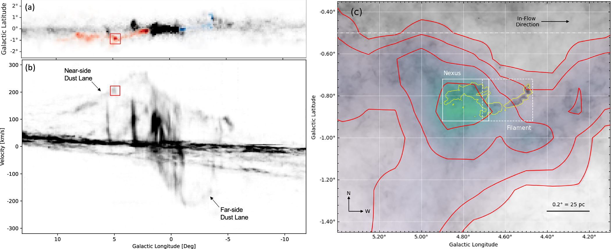
Figure 1. Panel (a): integrated 12CO (1–0) emission from the T. M. Dame et al. (2001) survey, toward the inner ∼25°of the Milky Way. Highlighted in red and blue are the Milky Way’s Galactic Bar Dust Lanes, near-side and far-side, respectively, from D. J. Marshall et al. (2008) and M. C. Sormani & A. T. Barnes (2019). Panel (b): position–velocity diagram of 12CO (1–0) for the emission shown in panel (a). Annotated in panel (b) are the near-side and far-side Dust Lane structures in position–velocity space. Red boxes in panels (a) and (b) show the location of the Midpoint (M4.7–0.8) of the Galactic Bar Dust Lanes in position–velocity space. Panel (c): 250 μm grayscale from Herschel (S. Molinari et al. 2016) with overlaid 12CO emission with red contours at 15, 25, 50, and 100 K km s−1 from M. C. Sormani & A. T. Barnes (2019), centered on the M4.7–0.8 cloud (red box in the left panel). The image opacity of the 12CO emission is scaled by the intensity. The solid white box shows the field of view (FOV) of the Green Bank Telescope (GBT) observations targeting the main “Nexus” of the cloud (pilot study), and the dashed white box shows the FOV of the GBT observations targeting the “Filament” of the cloud (DDT). The light yellow contour in panel (c) shows the GBT NH3 (1,1) emission at 15σ (150 mK, Figure 2). The dotted–dashed line shows the b = −0 5 orientation—the lower Galactic latitude limit of many Galactic plane surveys (e.g., SEDGISIM, HOPS; F. Schuller et al. 2021 and C. R. Purcell et al. 2012, respectively). A compass for the cardinal directions in the Galactic coordinate system is shown in the bottom-left corner of panel (c).
Download figure:
Standard image High-resolution image1.1. M4.7–0.8: The Midpoint of the Near-side Galactic Bar Dust Lane
The midpoint of the near-side Galactic Bar Dust Lane is observed to be one of the brightest regions observed in the 12CO data set (Figure 1(a), highlighted by the red box). Based on the geometrical model presented in M. C. Sormani & A. T. Barnes (2019), the Midpoint is located at R/Rbar ∼ 0.5, at a distance of 7.0 kpc (we discuss this 3D geometry in more detail in Section 5.1). Gas located at the midpoint is observed to have a line-of-sight velocity of ∼200 km s−1 (Figure 1(b); R. Fux 1999; D. J. Marshall et al. 2008; M. C. Sormani & A. T. Barnes 2019). Based on previous work from M. C. Sormani & A. T. Barnes (2019), the 12CO at this location is estimated to have a mass of ∼106 M⊙ and is suggested to accrete into the CMZ in 5–6 Myr, potentially forming a Sgr B2-like complex after CMZ accretion. This accretion is in the Westward direction for the near-side Dust Lane (see Figure 1(c)), indicating the plane-of-sky velocity is also Westward. Figure 1(c) shows the 12CO contours overlaid on the Herschel 250 μm dust continuum. The solid white box denotes the region we will be referring to as the “Nexus” in this paper. The Nexus coincides with the brightest 12CO emission and appears correlated with the nexus of the dust continuum and 12CO emission. The dashed white box highlights the feature we will be referring to as the “Filament.” This narrow dust continuum feature appears to be an extension off of the Nexus of the cloud and shows a filamentary morphology.
In this paper, we target these two fields (white boxes in Figure 1(c)) of the midpoint region of the Galactic Bar Dust Lanes using the Robert C. Byrd Green Bank Telescope (GBT). We target multiple transitions of ammonia (NH3) and cyanobutadiyne (HC5N) to investigate the higher-resolution molecular gas morphology and kinematics of this region. We discuss the observations and data reduction in Section 2. We present the detection of dense gas in these observations in Section 3 and analyze the morphology and kinematics of the cloud. We compare our dense gas observations to previous dust continuum studies in Section 4. Lastly, we investigate the 3D location, star formation, and other cloud properties in Section 5. We summarize these conclusions in Section 6.
2. Observations and Data Reduction
The data presented in this paper were taken using the 100 m GBT,12 located at the Green Bank Observatory in Green Bank, West Virginia. These single-dish radio observations were taken using the 18–26.5 GHz K-band Focal Plane Array (KFPA) receiver (∼31″ angular resolution; ∼1 pc at the assumed distance to the Galactic Bar).
An initial study targeted a single 0 25 × 0
 25 field centered at the location of strong CO emission associated with the midpoint of the near-side Dust Lane (see Figure 1(c)). Preliminary results indicated that a filamentary structure, visible in 250 μm emission toward lower Galactic Longitudes, was also associated with NH3 emission detected in this preliminary field. Additional observations were therefore proposed and completed in order to extend the original field over the range of this filament.
Fully sampled maps were completed using the 7 pixel KFPA on the GBT, centered at rest frequencies of 23.695, 23.723, 23.870, 24.139, and 24.533 GHz. These frequencies relate to the J = K = 1–513 rotational inversion transitions of the NH3 molecule. A further rest frequency of 23.964 GHz was also observed, matching the HC5N (9–8) rotational transition. Observations took place over eight sessions from 2020 April 3 to 2024 February 19.
2.1. Observational Setup
The seven beams of the KFPA were used for simultaneous, dual circular-polarization observations over the ∼3 footprint of the receiver. Flux calibration was achieved via off-source “blank-sky” and switched noise-diode measurements, resulting in an estimated antenna temperature accuracy of ∼20%. Atmospheric opacity values were determined from NWS grid values using a combination of three local sites, depending upon the established weather conditions (i.e., wind direction and agreement between the sites) at the time of observation. The VEGAS spectrometer backend was used in mode 20 (23.44 MHz, 200 km s−1, bandwidth per spectral window with 5.7 kHz, 0.07 km s−1, spectral resolution). Table 1 shows the line and imaging information (e.g., rest frequency, angular resolution) for the spectral lines presented in this study. More information on the imaging stage of the data reduction is discussed in Section 2.3.
Table 1. List of Targeted Lines
| Line Properties | Image Properties | |||
|---|---|---|---|---|
| Spectral | Rest | Beam | rms | Peak |
| Line | Frequency | Size | Noise | Intensity |
| (GHz) | (″) | (mK) | (K) | |
| NH3 (1,1) | 23.6944955 | 31.34 | 10 | 1.06 |
| NH3 (2,2) | 23.7226333 | 31.30 | 10 | 0.81 |
| NH3 (3,3) | 23.8701292 | 31.11 | 10 | 2.04 |
| NH3 (4,4) | 24.1394163 | 30.75 | 10 | 0.37 |
| NH3 (5,5)a | 24.5329887 | 30.27 | 10 | 0.22 |
| HC5N (9-8) | 23.9639007 | 30.99 | 10 | 0.17 |
Note. aThis transition was only observed in the Filament region and is therefore not used in the analysis of this paper beyond stating the detection. The NH3 (5,5) transition is shown in the Appendix A.
Download table as: ASCIITypeset image
2.2. Mapping and Observing Strategies
Maps were performed via an on-the-fly process with Nyquist-sampled rows in Galactic longitude. The “Off” positions were observed at intervals corresponding to the observation of four complete map rows. This allowed for sky emission compensation on a timescale of ∼10 minutes, adequate for observations at the K band. Due to the high level of extended emission in directions toward the GC, large position offsets were necessary in order to ensure emission-free “Off” measurements. These offsets were typically 5° and 3° in longitude and latitude, respectively. Pointing and focus calibrations were performed at the beginning of each observing session and approximately hourly thereafter.
2.3. Data Reduction
Data were reduced primarily using the GBTIDL package (P. Marganian et al. 2006).14 The “Off” position measurements were found to be stable over the duration of each individual session and so were averaged together in order to provide increased signal-to-noise ratio (SNR) in the final reduction. Each individual Nyquist-sampled integration was smoothed via a Gaussian convolution function. The resulting spectral resolution is 0.7 km s−1. The “Off” spectra were further smoothed to a resolution of 0.84 km s−1 before being subtracted from the reference spectra and scaled via the system temperature determined from the “flickered” noise-diode measurements. Atmospheric corrections (found as described above) were applied in order to place our data on the corrected antenna temperature (TA*) scale.
An initial spectral baseline was fit to emission-free regions of each integration using orthogonal polynomials of the order of 7. The subsequent output was then gridded via the gbtgridder15 routine using a Gaussian imaging kernel and a pixel width of 9″, approximately one-third of the observed beam size. The FITS cubes resulting from each session were examined individually on the basis of rest frequency as well as on the individual KFPA beam/feed used. In some cases, it was found that individual beams were unstable and/or contributing significantly higher levels of system noise. Where this was found to be detrimental to image quality, these beams were excised from the overall reduction.
It was found that, over three observing sessions performed on the “filament” section of our overall region, there were significant disagreements in the positional metadata of our maps. This resulted in considerable differences in the antenna temperature measurements when compared pixel-to-pixel. It is believed that this problem arose as a result of poor elevation pointing calibration of the GBT, below elevations of ∼20°.16 This was addressed in our data via careful examination of pointing offset data from peak scans and corrective offsets being applied to those data before gridding. The maps performed during the pilot phase of the study showed no evidence of this issue. Therefore, we are confident in the astrometry of those maps as a reference and determine our pointing accuracy to be the same as our pixel width, 9″. Following the final combination of data from all individual sessions, a final baseline removal process was applied to each cube as a whole. This was done using a polynomial function fit to emission-free regions. The order of the polynomial fit was chosen to be as low as necessary to remove any obvious “ripple” structure on the scale of the spectral window (23.44 MHz). For the NH3 (1,1), (3,3), (4,4), and (5,5) lines, this was determined to be a third-order polynomial. For the NH3 (2,2) and HC5N transitions, this was found to be second and fifth order, respectively. No direct correlation was found between the level of sinusoidal variation in a transition’s bandpass and any known hardware properties. System temperatures and measured rms noise values were largely consistent across all observed frequencies.
3. Detection of Dense Molecular Gas at the Midpoint
We have detected dense gas, as traced by the NH3 and HC5N molecules, at the midpoint of the Galactic Bar Dust Lanes: the M4.7–0.8 molecular cloud.17 In the following sections, we discuss the morphological structure (Section 3.1) and the gas kinematics (Section 3.2) of the molecular gas in this region. As we will show in Section 3.2, M4.7–0.8 has a central velocity ∼200 km s−1, consistent with values for the midpoint (Figure 1(b)). Therefore, we will assume a distance of 7.0 kpc, with a conservative error estimate of 1 kpc, for all physical size calculations. This 1 kpc error estimate is similar to those used in A. Nilipour et al. (2024), who argued for a thick dust lane and use this value in their error estimate as well.
3.1. Structure of the Dense Molecular Gas in M4.7–0.8
Figures 2 and 3 show the maximum emission in the NH3 (1,1)–(4,4) and the HC5N (9−8) transitions in the M4.7–0.8 molecular cloud.18 The NH3 (3,3) transition is the brightest out of all of our detected spectral lines, with a peak emission of 2.04 K (>200σ; Table 1). The HC5N (9–8) transition is the faintest of our detected spectral lines, with a peak of 0.17 K (17σ; Table 1).
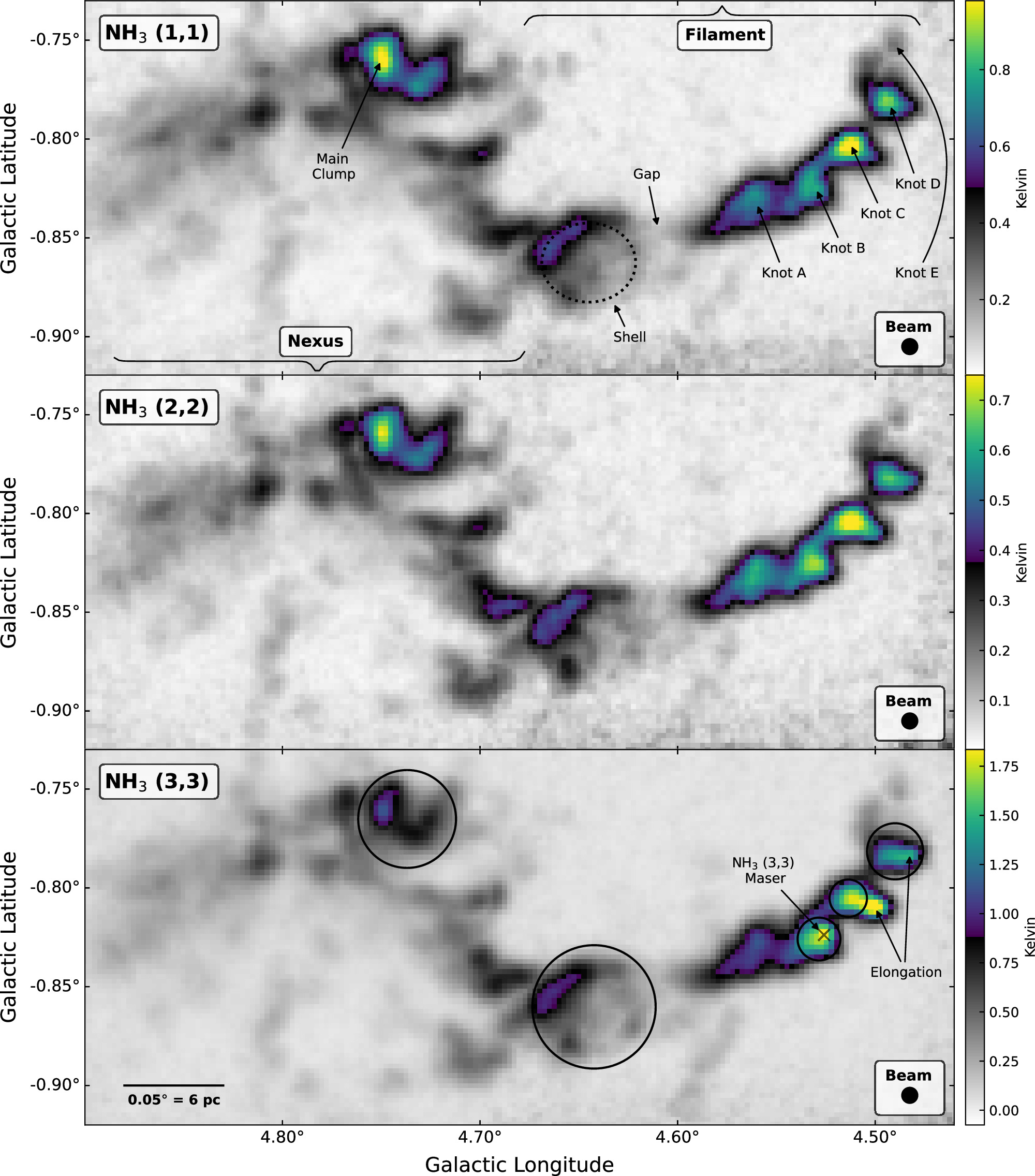
Figure 2. Peak antenna temperature for the NH3 (1,1)–(3,3) transitions, top to bottom, respectively, as indicated in the top-left corner. Annotated on the top, NH3 (1,1), panel are several features and sources discussed in Section 3, including the “Main Clump” in the Nexus and the “Gap” and “Knots” A–E in the Filament. The black dashed ellipse illustrates the region we are annotating as the “Shell.” The black “ × ” symbol in the NH3 (3,3) bottom panel shows the location of the NH3 (3,3) maser, discussed in Section 3.2.2. The beam size is shown at the bottom-right corner of each panel (see Table 1 for these values). A scale bar for the M4.7–0.8 cloud is shown in the bottom left of the NH3 (3,3) panel, assuming a distance of 7.0 kpc. The NH3 (3,3) panel also shows the apertures used to extract the spectra, shown in Figure 4, for regions: Main Clump, Shell, and Knots B–D (left to right, respectively). The knot elongation, observed in Knots C and D, in the higher J NH3 transitions, is annotated in the (3,3) panel.
Download figure:
Standard image High-resolution image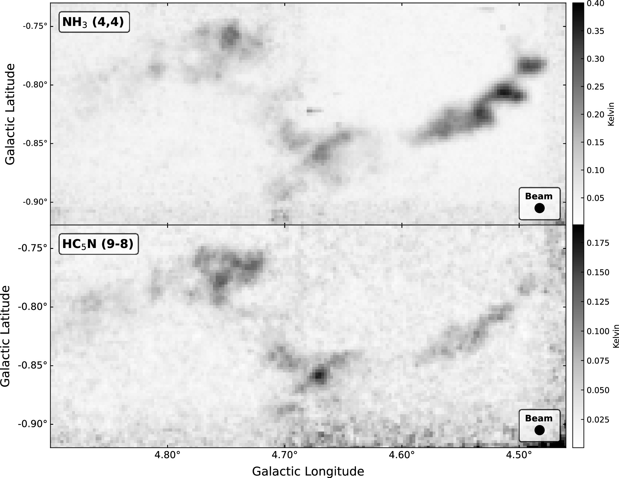
Figure 3. Peak antenna temperature for the NH3 (4,4) and HC5N (9–8) transitions, top and bottom, respectively (as labeled in the top-left corner). The beam is shown in the bottom-left corner. The beam size is shown in bottom-right corner (see Table 1 for these values). The noise floor in the Filament field is more prominent in these images, when compared with the NH3 (1,1)–(3,3) lines in Figure 2, due to the relatively low signal-to-noise ratio (SNR) detection influencing the scaling of these images.
Download figure:
Standard image High-resolution imageThe dense molecular gas at the midpoint of the Galactic Bar Dust Lanes (M4.7–0.8) is observed to be extended in Galactic Longitude (∼0 45, ∼55 pc) and contains several bright clumps that are unresolved in these GBT observations (∼30″, ∼1 pc; a scale bar is shown in Figure 2, bottom). The large-scale structure is fairly consistent across all observed transitions, showing a similar morphology in all five spectral lines (Figures 2 and 3). However, when looking at the localized morphology in the cloud, we can observe interesting substructures. These features are annotated in the top NH3 (1,1) panel of Figure 2, and they will be discussed throughout this paper.
As mentioned previously in this paper, we highlight two main regions in the cloud: a “Nexus” (the region associated with the 12CO peak) and a “Filament” (the dust continuum filament extending out from the Nexus). The Nexus contains several faint, diffuse, extended structures (0 05–0
05–0 15), with a main bright clump located at l = 4
 74, b = −0
 76, labeled as “Main Clump” in Figure 2.
The Filament is generally long (∼0 3, ∼40 pc) and narrow (∼0
 03, ∼4 pc), resulting in a length-to-width ratio of roughly 10. While generally observed to be one continuous structure, we note a small discontinuity, labeled as the “Gap” (Figure 2; l = 4
 61, b = −0
 85), where the emission is relatively faint when compared with adjacent sections of the Filament. This decrease in emission at this location in the structure is observed across all five transitions. On the eastern side of the Gap, there is a shell-like structure, labeled as the “Shell,” which shows a brighter curved rim and a fainter cavity (dotted black line in Figure 2). The Shell appears to be brightest on the eastern rim with very low level emission on the western rim.
On the western-most region of the Filament, we observe five bright knots of emission in the NH3 transitions, labeled as Knots A–E in Figure 2. These sources are roughly evenly spaced, with a separation of ∼2 (4.4 pc) between adjacent knots. While bright in the NH3 transitions, we do not observe evidence of these knots in the HC5N line above 125 mK (∼12σ)—only in the large-scale structure of the Filament. Knot C is observed to be the brightest in every NH3 transition, including the NH3 (5,5) transition (Figure A1). Knot E is observed to be the faintest in our observed transitions, and is only faintly detected in the J ≤ 4 transitions. Knot E is also observed to be smaller (r = 20″; 0.7 pc) than Knots A–D and is unresolved in these observations.
Knots B, C, and D exhibit some similar characteristics when comparing the NH3 (1,1) to NH3 (3,3) emission. Here, the NH3 (1,1) emission describes condensed circular emission peaks, which are toward the northern edge of the Filament. In comparison, the NH3 (3,3) emission has a more extended morphology, with the NH3 (1,1) peaks occurring toward the eastern end of each respective prolate knot. This elongation in the higher J transitions is annotated in the bottom panel of Figure 2. It should be noted that this is true for emission measured in the NH3 (4,4) and (5,5) transitions as well (Figures 3 and A1, respectively). We also note that this is true for emission measured both as the peak temperature as well as the integrated intensity of the respective NH3 transitions, as we will illustrate in the next section in our kinematic analysis.
3.2. Kinematics of the Dense Molecular Gas in M4.7–0.8
In our study of the near-side Dust Lane, we not only seek to determine the gas structure of the observed region, as discussed in Section 3.1, but also aim to establish the bulk motions within that gas. Whether it is possible to confirm the transport of material along the Dust Lane with the presented data or to investigate any potential structural developments within the cloud as a single element, it is useful to examine the dynamic state of the observed gas. Here we present a kinematical analysis of the dense gas in the surveyed region using a thorough inspection of the observed spectra as a function of position.
The simplest way to investigate gas kinematics is by extracting spectra. We selected five regions to investigate: the Main Clump, the Shell, and Knots B, C, and D. The apertures used to extract the spectra for each region are shown as black circles in Figure 2.19 The spectra were then extracted and plotted in Figure 4 using the python programs SpectralCube20 and pyspeckit21 (A. Ginsburg et al. 2022).
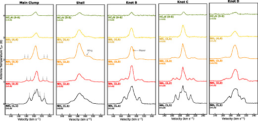
Figure 4. Integrated spectra of the NH3 (1,1)−(4,4) and HC5N (9−8) lines in the M4.7–0.8 cloud for the five apertures shown in Figure 2, with the label of the aperture shown on the top of each panel. Each spectrum is labeled by its corresponding transition on the left side of the plots. Several spectra have been scaled for visualization purposes. These spectra are denoted with the value used for this scaling below the transition name on the left side of the plot. The gray arrows in the first panel (Main Clump) show the location of the hyperfine satellite lines for the NH3 (1,1)–(3,3) transitions. The hyperfine lines are not noticeable in the (4,4) spectrum and are therefore not shown. The asymmetric “wing” in the spectral line profile, discussed in Section 3.2, is annotated in the Shell panel—where the offset in the secondary component is the most noticeable. The NH3 (3,3) maser, detected in Knot B, is annotated with a gray arrow in the middle panel.
Download figure:
Standard image High-resolution imageThe NH3 molecule has a known hyperfine structure containing four primary satellite lines that are offset from the main component (e.g., P. T. P. Ho & C. H. Townes 1983, gray arrows in the leftmost panel of Figure 4). These satellite lines are clearly detected in the (1,1)–(3,3) transitions. However, drawing upon the (1,1) transitions as an example, we can see that the inner satellite lines are blended with the main component in all of the extracted spectra. It can be seen that the outer satellite lines are also not clearly separated, particularly in the cases of the Shell and Knot D. We attribute this blending to the particularly large linewidths seen in this region and discuss this further in Section 3.2.1. The NH3 (3,3) line in the Knot B region shows a narrow-line component around 195 km s−1 that is not observed in any of the other regions (Figure 4). This feature appears to be contained to the area marked with the black “ × ” in Figure 2. This narrow-line velocity feature could be associated with NH3 (3,3) maser emission and is discussed in detail in Section 3.2.2. Several of the profiles show “wings” in the main profile component, as annotated in the Shell panel of Figure 4, suggesting a secondary component offset in velocity. This secondary component is most visible in the Shell profile, but is also present in the Main Clump and Knot B (Figures 4 and 5).
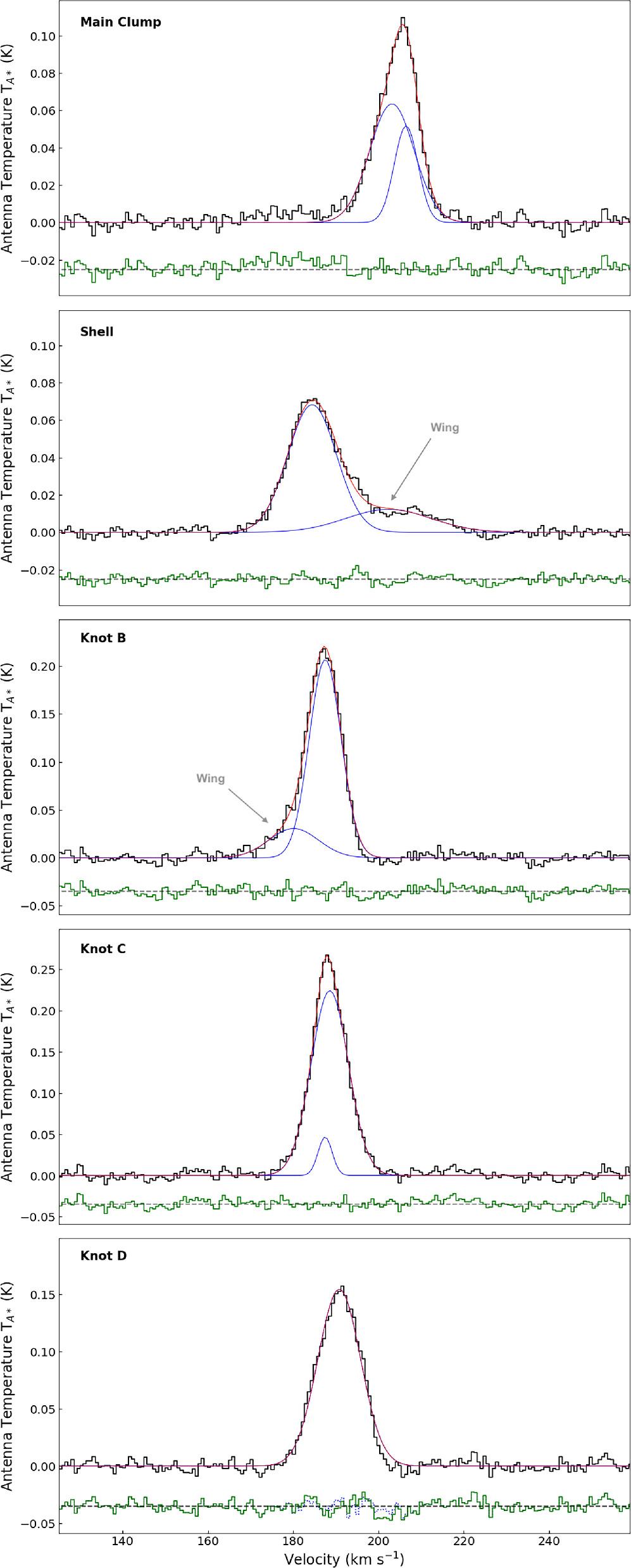
Figure 5. Fitted spectra of the NH3 (4,4) line. The red line shows the best Gaussian fit to the extracted spectra (black line). The green line shows the residuals from the best fit. The blue profiles show the individual Gaussian components. The fit parameters are presented in Table 2.
Download figure:
Standard image High-resolution imageThe hyperfine structure of NH3 molecular emission has been used in many studies to extract valuable information on the physical properties (primarily temperature and optical depth/column density) of the regions under examination (e.g., GAS, KEYSTONE, RAMPS; R. K. Friesen et al. 2017; J. Keown et al. 2019; T. Hogge et al. 2018, respectively). However, due to the line blending seen here, such analysis is particularly complicated and may even be impossible (or so degenerate as to be inconclusive). In this publication we are only focusing on the gas morphology and kinematics and will therefore not be using the hyperfine lines in our analysis. A follow-up publication will investigate the hyperfine lines in more detail. Thus, we have chosen to use the (4,4) transition as the primary line from which to extract the basic velocity parameters (e.g., vc, σ) of our observations.
Figure 5 shows the NH3 (4,4) line profile for these regions (black histogram), fit with 1–2 Gaussian components (blue profiles) using the python program pyspeckit. The parameters for these fit components are shown in Table 2. Most of the spectra are best fit with two Gaussian components with the exception of Knot D, for which a single component is optimal. The solid green line, offset at −0.025 K in all panels, shows the residual of the best-fit line profile, shown as the red line in Figure 5. A secondary residual (blue dotted line) is shown for Knot D, for which there is slight improvement in the fit if a secondary component is included. This improvement in the residuals is best seen around 200 km s−1. However, as this improvement is at the 1σ level of the noise, we will examine this source using the single Gaussian fit.
Table 2. Kinematics of the NH3 (4,4) Transition
| Parametera | Value |
|---|---|
| Main Clump | r ∼ 89 1 (3.46 pc) 1 (3.46 pc) |
| Ac | 64 ± 7 mK |
| vc | 203.1 ± 0.4 km s−1 |
| σ | 5.2 ± 0.1 km s−1 |
| Ac | 52 ± 8 mK |
| vc | 206.5 ± 0.2 km s−1 |
| σ | 2.8 ± 0.3 km s−1 |
| Shell | r ∼ 112 4 (4.36 pc) 4 (4.36 pc) |
| Ac | 68 ± 7 mK |
| vc | 184.4 ± 0.1 km s−1 |
| σ | 5.7 ± 0.1 km s−1 |
| Ac | 12 ± 1 mK |
| vc | 202.3 ± 1.5 km s−1 |
| σ | 10.0 ± 1.2 km s−1 |
| Knot B | r ∼ 39 0 (1.51 pc) 0 (1.51 pc) |
| Ac | 207 ± 26 mK |
| vc | 187.5 ± 0.2 km s−1 |
| σ | 3.7 ± 0.2 km s−1 |
| Ac | 31 ± 12 mK |
| vc | 180.1 ± 4.5 km s−1 |
| σ | 5.8 ± 2.1 km s−1 |
| Knot C | r ∼ 34 1 (1.32 pc) 1 (1.32 pc) |
| Ac | 224 ± 8 mK |
| vc | 188.6 ± 0.1 km s−1 |
| σ | 4.4 ± 0.1 km s−1 |
| Ac | 47 ± 8 mK |
| vc | 187.5 ± 0.2 km s−1 |
| σ | 1.7 ± 0.3 km s−1 |
| Knot D | r ∼ 51 1 (1.98 pc) 1 (1.98 pc) |
| Ac | 154 ± 2 mK |
| vc | 190.8 ± 0.1 km s−1 |
| σ | 5.0 ± 0.1 km s−1 |
Note. aAc is the amplitude of the fit, vc is the central velocity of the component, and σ is the velocity dispersion. The r parameter on the same line as each of the region names defines the radii value of that region. Region names are in bold.
Download table as: ASCIITypeset image
Most of the measured velocity dispersion values are between 2 and 5 km s−1 (Table 2). The largest velocity dispersion measured in our spectra is associated with the Shell (10.0 ± 1.2 km s−1). Knot D is best fit with a broadest single component spectrum (5.0 ± 0.1 km s−1). Knot C is the brightest of the five regions shown here. The offset in the secondary velocity component is the most extreme in the Shell and Knot B, with velocity offsets >5 km s−1. These lower-intensity velocity components, discussed previously as “wings,” are annotated in these two panels of Figure 5.
Due to the hyperfine structure of the NH3 molecule, analysis of the kinematics can be quite complex because of the satellite lines. These hyperfine lines become much more prominent at the lower transitions (e.g., Figure 4). Therefore, we will be using the NH3 (3,3) line for the kinematic analysis for the following arguments. First, the emission in the (3,3) line is relatively bright when compared with the (1,1) line (see Figure 2). Second, hyperfine satellite lines in the (3,3) transition are relatively faint compared to the main component. These strong hyperfine lines in the (1,1) and (2,2) transitions are visible in Figure 4. Although the hyperfine lines in the (3,3) transition are visible in Figure 4, the ratio of the hyperfine lines to the main component is lower than the (1,1) and (2,2) transitions. Third, the larger velocity offset between the satellite lines and the main component allows for better isolation of the main component in velocity space. We note in later sections where the analysis could be influenced by the lower-level hyperfine emission. And lastly, while the HC5N (9–8) transition would be an excellent candidate to use for kinematic analysis, due to the lack of hyperfine structure in the line profile, the relatively low SNR makes fitting the velocity components across the structure unfeasible. Although the NH3 (4,4) line was used for the spectral line analysis, discussed earlier in the section and shown in Figure 5, the relatively faint nature of this transition on a pixel-by-pixel analysis (e.g., see the maximum intensity emission shown in Figure 3) makes this transition unfeasible to use in the “moment” analysis in the following section.
3.2.1. Central Velocity and Velocity Dispersion
In this section, we use the NH3 (3,3) data to investigate the gas kinematics in the cloud by creating moment 0 (M0, integrated intensity), moment 1 (M1, central velocity), and moment 2 (M2, velocity dispersion) maps. These moment maps are defined by the following equations:


and

where  is the antenna corrected temperature of the data cube in kelvin, and v is the velocity in kilometers per second. These types of visualizations can illustrate velocity gradients across the source and can reveal regions with high velocity dispersion. However, care is needed when viewing these images—especially in cases where hyperfine lines are strong or multiple components are present. Figure 6 shows these three moment images, discussed above, for the NH3 (3,3) line.
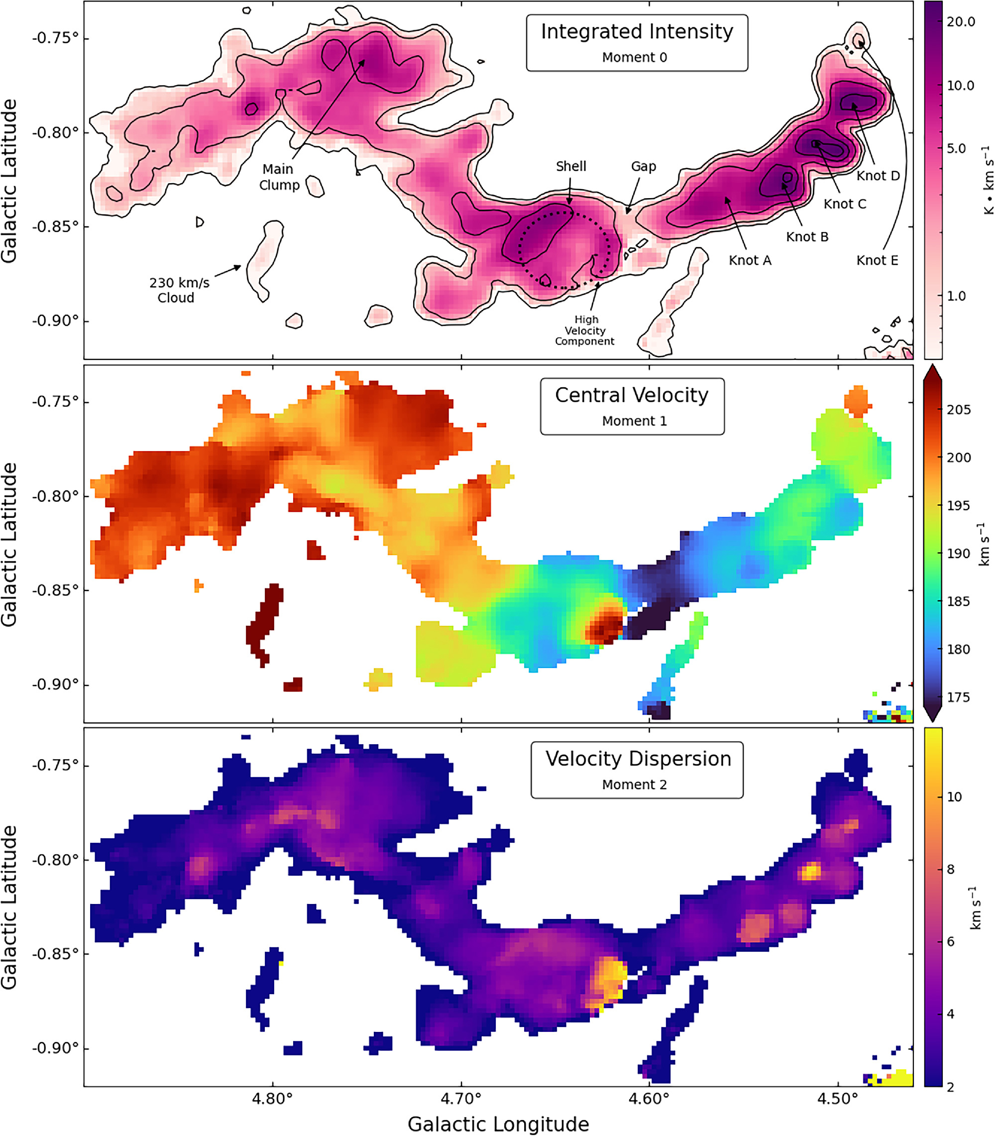
Figure 6. Integrated intensity (Moment 0; top panel), central velocity (Moment 1; middle panel), and velocity dispersion (Moment 2; bottom panel) for the NH3 (3,3) transition in the M4.7–0.8 cloud. Contours on the integrated intensity (top panel) show the 15, 25, 60, 120, and 175 × 10 mK peak intensity (rms noise). All three panels use a lower limit cutoff of 150 mk (15σ; lowest level contour in the top panel). Annotated in the top panel are the features discussed in Section 3.
Download figure:
Standard image High-resolution imageAll three moment maps shown in Figure 6, M0–M2, were created in CASA (CASA Team et al. 2022), using the immoments command. We used a robust lower limit cutoff of 150 mK (15σ) for all three moments to avoid fitting noise components in our integration. We used a velocity range of 146.4–257.8 km s−1 when making these images.
The NH3 (3,3) integrated emission (Moment 0; Figure 6, top) generally traces a distribution similar to that of the NH3 (3,3) peak intensity (Figure 2, bottom). As noted previously in Section 3.1, the elongation observed in the peak emission in Knots B–D is also observed to be present in the integrated emission as well. The NH3 (3,3) central velocity (Moment 1; Figure 6; middle panel) shows that velocities in the cloud generally range between 180 and 210 km s−1. This velocity range is consistent with values expected for the midpoint of the dust lanes (∼200 km s−1; see Figure 1(b)).
In general, the Nexus has slightly higher velocities, around 195−210 km s−1, when compared to most of the emission in the Filament (180−195 km s−1). This subtle velocity distribution (∼15 km s−1) across the broad ∼60 pc structure results in a large-scale velocity gradient across the M4.7–0.8 cloud of ∼0.25 km s−1 pc−1, from east to west.
Within the Nexus region of the M4.7–0.8 cloud, there are no broad-scale velocity gradients. There are a few localized gradients of a few kilometers per second associated with emission across adjacent cloud clumps. South of the bulk emission in the Nexus is an elongated vertical clump that is labeled as the 230 km s−1 cloud in the top panel of Figure 6. This feature is oversaturated in the M1 map (Figure 6, middle panel) and is a distinct component along our line of sight. This feature is also observed to be a discrete component in position–velocity space (see Figure B2 and Appendix B.3 ).
The Filament shows a more complex velocity structure compared with the Nexus. Toward the “Gap” in the Filament (annotated in Figure 6, top) we observe the lowest velocity across the entire cloud, with velocity values extending down to 175 km s−1. There is a generally increasing velocity gradient away from the “Gap” location in both directions along the Filament. Adjacent to the “Gap,” near the western rim of the “Shell,” we observe the highest velocity associated with the Filament (210–215 km s−1), which we have labeled as the “high-velocity component.” In the Moment 1 map, in the region between the high-velocity component and the Gap, we observed a sharp jump in the central velocity across a few pixels. This type of discontinuity in the velocity distribution typically occurs when two components are located along the same line of sight. In this case, the central velocity in the fitting algorithm is shifted by bright emission in one component compared with the other (see Equation (2)) across a few pixels. This higher-velocity emission appears to be constrained to the western rim of the Shell, suggesting this feature is likely a secondary component along the line of sight. Furthermore, the high-velocity component is observed to be a distinct feature in the position–velocity diagram (Figure B2) and in channel maps (Figure B3)—both of which are discussed in Appendix B. This high-velocity component is likely the secondary profile observed in the Shell spectrum (10 km s−1; Figure 5, Table 2). As the spectrum shown in Figure 5 is from the NH3 (4,4), and therefore from the same NH3 molecule shown in Figure 6, they are likely tracing the same velocity components.
The general velocity gradient in the Filament is clear, with an increasing velocity from Knot A (∼180 km s−1) to Knot E (200 km s−1).22 Knots B and C show a velocity gradient across the elongated knot substructure. In these two sources, we also observe a velocity gradient from the northeast to the southwest. In the northeast, the emission is higher, around 190 km s−1, whereas in the southwest the emission lower, around 183–185 km s−1. This results in a velocity gradient across the substructure of 2.5 km s−1 pc−1. Knot E is observed to have the highest velocity and appears distinct from its neighbor, Knot D.
The NH3 (3,3) velocity dispersion (Moment 2; Figure 6, bottom) in the M4.7–0.8 cloud is generally around 2–10 km s−1. The periphery of the cloud is observed to have lower velocity dispersion (≤2 km s−1), whereas the interior of the cloud is observed to have higher velocity dispersion (∼6 km s−1). There are a few clumps where the velocity dispersion exceeds 10 km s−1. The high-velocity component is observed to be one of these regions. This high velocity dispersion is consistent with the spectral fitting results for the secondary component in the Shell (Table 2).
However, many of these other clumps with large velocity dispersion values have prominent hyperfine lines. Due to the approach in which CASA calculates the velocity dispersion, by using a simple, single Gaussian fit, satellite lines can result in a broadening of the velocity dispersion in regions with relatively bright hyperfine lines. While the hyperfine lines are suppressed in the (3,3) transition when compared with the (1,1) line (see Figure 4), regions where the hyperfine line is quite strong can result in high apparent velocity dispersion values in Moment 2 maps. Knot C is one of these regions which shows relatively high velocity dispersion in the Moment 2 map, but an examination of the (3,3) profile for this region reveals relatively strong hyperfine lines that are likely causing the high dispersion values in this plot. Here we take the presented dispersion values, in Figure 6, as illustrative and reserve a full analysis of the individual hyperfine component velocity dispersions for a future publication.
3.2.2. Detection of a New NH3 (3,3) Maser
A narrow-line velocity feature is observed in the NH3 (3,3) spectral cube at l = 4 53, b = −0
 82 (see black “×” in Figure 2), and is clearly visible in Figure 4 (Knot B, NH3 (3,3) panel), and Appendix B Figures B2 and B3. The location of this narrow-line emission feature suggests it is associated with the northwestern region of Knot B. Bright, narrow-line profiles in the NH3 (3,3) are often indicative of maser emission (e.g., J. G. Mangum & A. Wootten 1994; K. E. Kraemer & J. M. Jackson 1995), supporting our identification of this feature as a new NH3 (3,3) maser detection.
For this analysis, we will be using an un-smoothed version of the data set. This data set was sampled at the native resolution of 0.07 km s−1, with no additional smoothing (see Section 2.3). This higher-resolution channel width is necessary to fully resolve and sample the narrow-line component associated with the maser emission. To better understand the nature of the source, we fit the NH3 (3,3) spectrum, shown in Figure 4, using the python program pyspeckit (A. Ginsburg et al. 2022). This package allows us to account for the prominent hyperfine components of the NH3 (3,3) transition when performing our fit. The raw NH3 (3,3) spectrum for Knot B is shown in Figure 7 as a black histogram. We fit this profile with a two-component fit, using similar central velocity and velocity dispersion values previously measured in the NH3 (4,4) data (see Table 2). We note that despite the higher spectral resolution of this data, compared with the spectrum used in Figure 5, we still recover the same components. The residuals from this two-component fit are shown as a dotted blue line at −0.25 K, in which the narrow-line feature is clearly detected. When adding an additional narrow-line component to our fitting algorithm, we can see that the residuals are greatly improved (solid green line at −0.25 K in Figure 7). The parameters of this three-component fit, with the combined fit shown as a red line in Figure 7, are presented in Table 3. The introduction of a fourth component, with a central velocity of 181 km s−1 and a broad velocity dispersion of ∼8 km s−1, can slightly improve the residuals in the fit around 180 km s−1. However, without additional evidence to support this fourth component, it is unclear whether this is an additional velocity component or the result of noise in the brightest emission channels. Higher-resolution observations are necessary to spatially disentangle these multiple components and determine whether a fourth component is indeed present in this region.
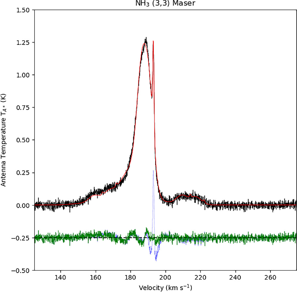
Figure 7. Spectrum showing the GBT NH3 (3,3) maser, using the native resolution data set (ΔV = 0.07 km s−1). The black line shows the raw data extracted from the Knot B region indicated in Figure 2. The red line shows the sum of the three components fitted with the ammonia wrapper in pyspeckit. The values for these three components are shown in Table 3. The solid green line shows the residuals from fitting all three components from Table 3. The dotted blue line shows the residuals of the fit excluding the narrow-line component (vc = 193.16 km s−1)—illustrating the maser line in the residuals.
Download figure:
Standard image High-resolution imageTable 3. Kinematics of the NH3 (3,3) Transition in Knot B
| Parametera | Value |
|---|---|
| Main Component | |
| vc | 188.42 ± 0.02 km s−1 |
| σ | 3.05 ± 0.03 km s−1 |
| Secondary Component | |
| vc | 181.88 ± 0.21 km s−1 |
| σ | 7.49 ± 0.09 km s−1 |
| Maser Component | |
| vc | 193.16 ± 0.01 km s−1 |
| σ | 0.37 ± 0.01 km s−1 |
Note. avc is the central velocity of the component, and σ is the velocity dispersion.
Download table as: ASCIITypeset image
4. Dust Emission in M4.7–0.8
In this section, we compare our NH3 radio observations (Section 3) to previous infrared and submillimeter survey data sets as a way of investigating the dust continuum emission associated with the dense molecular gas. Figure 8 shows the submillimeter (870 μm) continuum from the Apex ATLASGAL survey (F. Schuller et al. 2009). The blue NH3 (1,1) contours clearly trace a similar structure in the submillimeter emission indicating the 870 μm continuum emission is correlated with the ∼200 km s−1 gas. The Main Clump in the Nexus and Knot D in the Filament are relatively bright at 870 μm. We also observe a brighter feature located toward the lower right of the NH3 (3,3) maser (yellow ×), as highlighted by the red box in Figure 8 (this annotated region will also be highlighted in Figures 9–10). We will discuss a multiwavelength analysis of this source in Section 5.3.1.
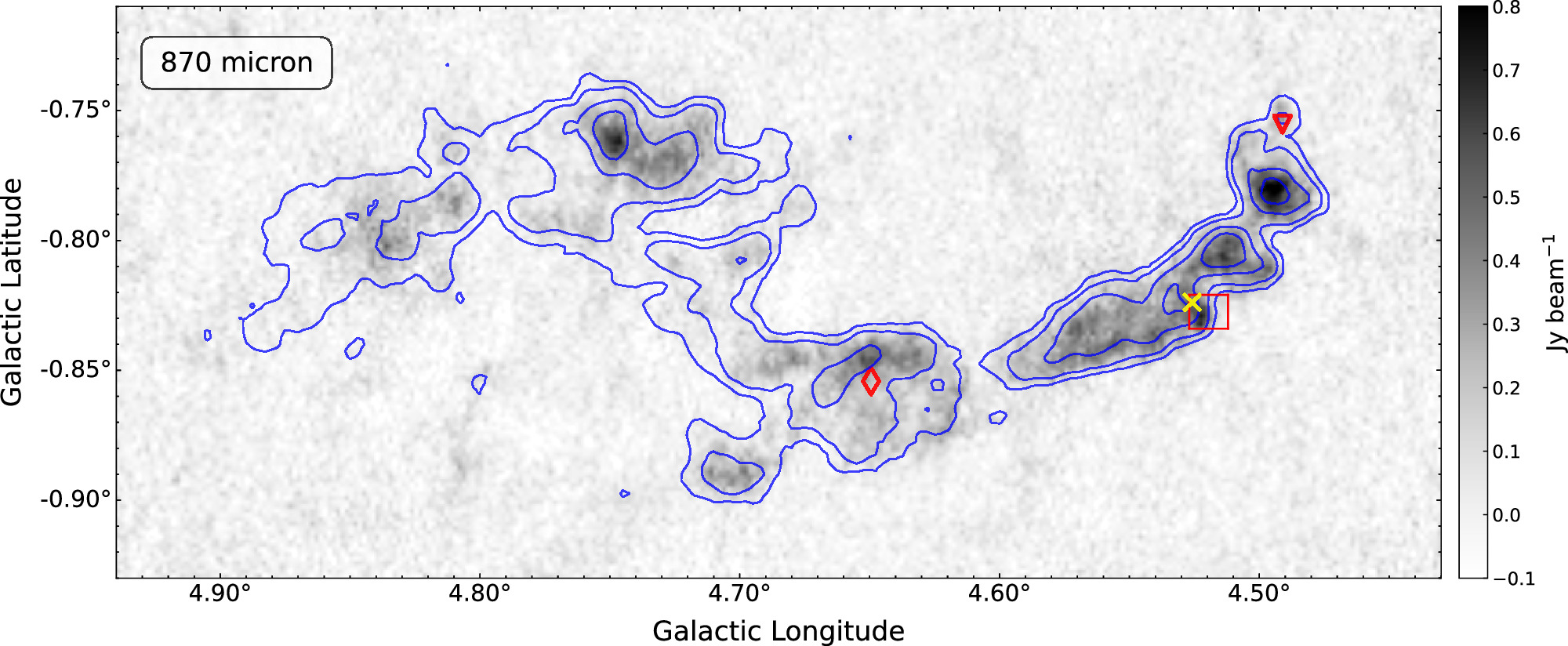
Figure 8. Submillimeter dust emission in the Midpoint cloud at 870 μm from ATLASGAL (18 2 resolution, 0.04 Jy beam−1 sensitivity; F. Schuller et al. 2009). Overlaid are the NH3 (1,1) peak emission at 0.15, 0.25, 0.5, and 0.75 K level contours (Figure 2). The yellow × symbol marks the location of the NH3 (3,3) maser (Section 3.2.2). The red diamond marks the location of the radio point source detected in the VLASS survey (M. Lacy et al. 2020; see Figure C1). The red triangle marks the location of the 70 μm point source from D. Elia et al. (2017). The red box shows the FOV region for the source targeted in Figure 14.
Download figure:
Standard image High-resolution image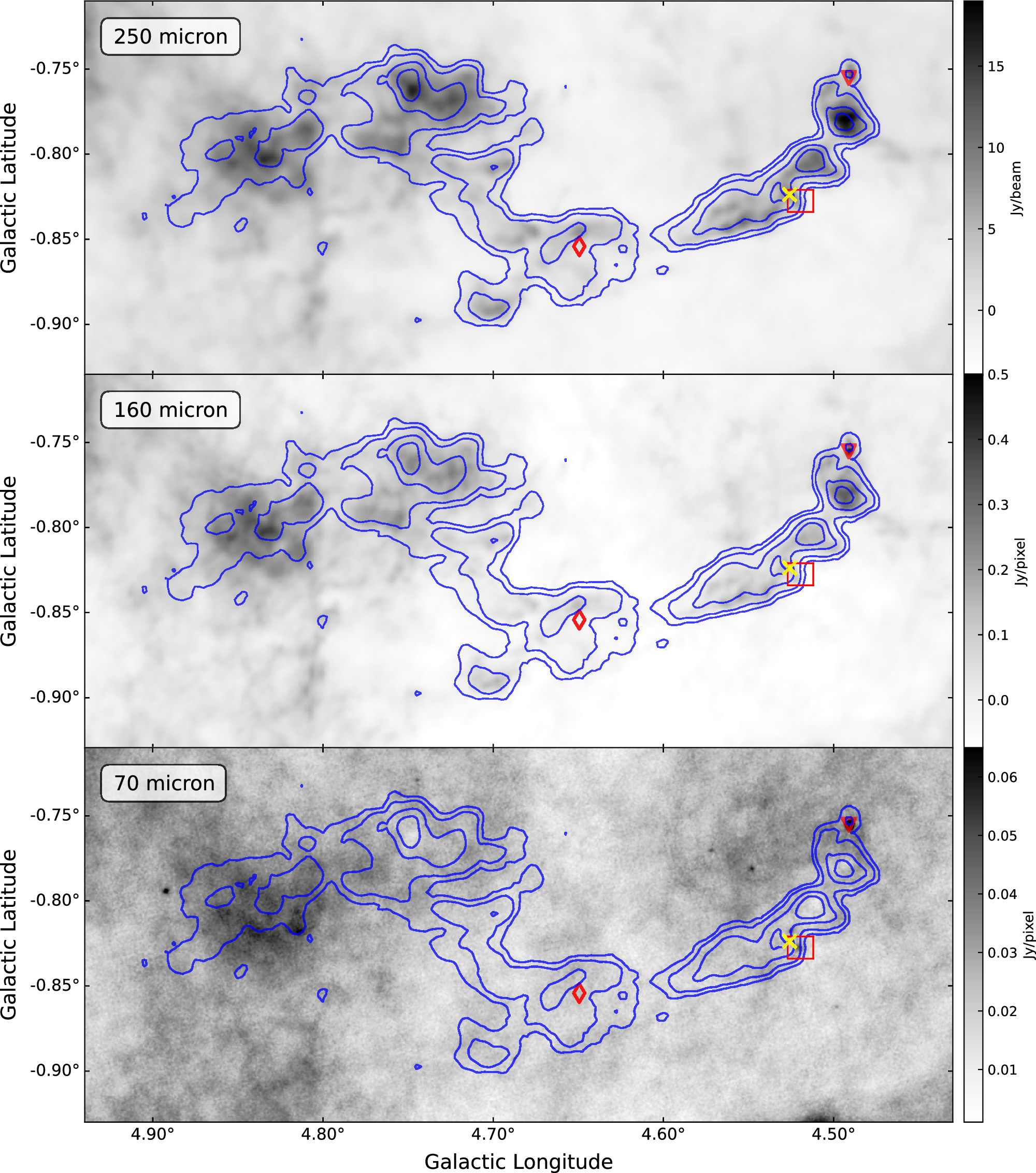
Figure 9. Far-infrared Herschel dust emission in the Midpoint cloud at 250 μm, 160 μm, and 70 μm (S. Molinari et al. 2016). The Herschel bands have a resolution of 6″, 3 2, and 3
 2 pixel−1 (top to bottom, respectively). The Herschel bands have a sensitivity of 0.2 Jy beam−1 (250 μm), 10 mJy pixel−1 (160 μm), and 4 mJy pixel−1 (70 μm). Overlaid are the NH3 (1,1) 0.15, 0.25, 0.5, and 0.75 K level contours from Figure 2. The yellow × symbol marks the location of the NH3 (3,3) maser, discussed in Section 3.2.2. The red diamond marks the location of the radio point source detected in the VLASS survey (M. Lacy et al. 2020; see Figure C1). The red triangle marks the location of the 70 μm point source from D. Elia et al. (2017). The red box shows the FOV region for the source targeted in Figure 14. A three-color image of these three data sets is shown in Appendix D (Figure D1).
Download figure:
Standard image High-resolution image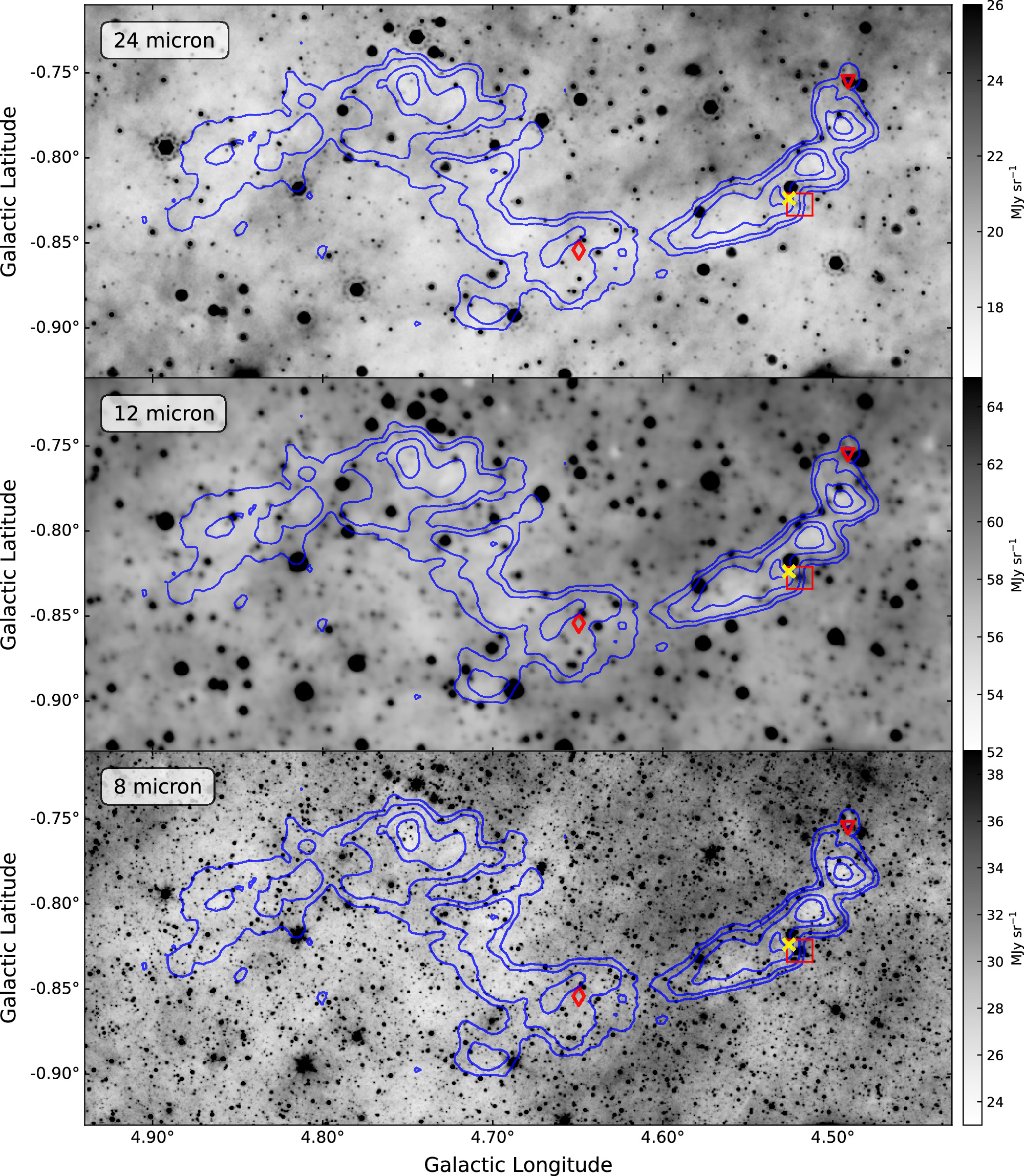
Figure 10. Mid-infrared Dust emission in the Midpoint cloud at 24 μm (MIPSGAL, 6″ resolution, 0.6 mJy beam−1; S. J. Carey et al. 2009), 12 μm (WISE, 6 5, 0.2 mJy beam−1; E. L. Wright et al. 2010), and 8 μm (IRAC-4, 1
 2, 0.4 mJy beam−1; E. Churchwell et al. 2009). Overlaid are the NH3 (1,1) at 0.15, 0.25, 0.5, and 0.75 K level contours from Figure 2. The yellow × symbol marks the location of the NH3 (3,3) maser, discussed in Section 3.2.2. The red diamond marks the location of the radio point source detected in the VLASS survey (M. Lacy et al. 2020; see Figure C1). The red triangle marks the location of the 70 μm point source from D. Elia et al. (2017). The red box shows the FOV region for the source targeted in Figure 14.
Download figure:
Standard image High-resolution imageFigure 9 shows the far-IR emission in three Herschel data sets from S. Molinari et al. (2016), at: 250 μm (top), 160 μm (middle), and 70 μm (bottom). The 250 and 160 μm emission show a somewhat similar emission distribution as the 870 μm emission (Figure 8), where we observe similar features (e.g., Main Clump in the Nexus, bright knots in the Filament). The 70 μm emission appears quite different from the 160 and 250 μm emission, with many of the extended emission features not detected at 70 μm.
The cloud appears to have two main dust components: one associated with the left side of the Nexus, and one associated with the Filament and the right side of the Nexus (see Figure D1). The left side of the Nexus is observed to be relatively faint in the 870 μm data (Figure 8) but increases in brightness toward the shorter IR wavelengths (Figure 9).
The right side of the Nexus and the region associated with the Filament are relatively bright in the 870 and 250 μm emission, but become relatively faint in the 160 μm emission, when compared with the left side of the Nexus. These emission regions are not observed in the 70 μm emission and in the case for the Main Clump and Knots C and D, they are observed to be somewhat extincted (Figure 9). The Gap in the Filament is also observed in the far-IR and submillimeter emission as well. As the Filament is not present in the 70 μm data, we do not detect the Gap in the 70 μm emission.
The 70 μm emission also appears to have several compact sources throughout the structure. The most notable of these is the compact source observed with Knot E (red triangle in Figure 8–10). This feature is discussed in more detail in Section 5.3.2. We also note a compact 70 μm source that coincides with compact emission observed in the 870 μm emission. This source is located in Knot B, near the NH3 (3,3) maser (yellow “ × ” in Figures 8 and 9). This compact feature does not appear to be detected in the 160 and 250 μm data sets. We will discuss this feature in more detail, later in this section.
Figure 10 shows the mid-IR wavelength emission at 24 μm (top; MIPSGAL), 12 μm (middle; WISE), and 8 μm (bottom; GLIMPSE). The mid-IR emission reveals the cloud to be an infrared dark cloud at short wavelengths due to the relatively low emission from within the cloud compared to the mid-IR background. Although this cloud is observed to be IR-dark, we can still observe hints of the same general structure as traced by the NH3 contours. This general structure is the clearest toward the Filament region, where we observe a sharp contrast between the Filament region and the background emission. The Nexus region shows a much more extended IR-dark region, indicating the dense gas, as traced by the NH3, is concentrated within this larger extinction feature. Furthermore, this extended region around the Nexus correlates with the bulk 12CO emission shown in Figure 1(c). We will discuss this extended component in the Nexus in more detail in Section 5.1.1. This lower-intensity mid-IR emission is strongest toward Knots C and D and the Main Clump of the cloud, indicating higher extinction in these regions. These are the same regions where we also observed 70 μm extinction (Figure 9, bottom). While this lower-level emission is the most extreme in these regions, all of the knots in the Filament show mid-IR extinction, including the most compact knot, Knot E. This higher extinction in these sources is likely due to the higher column densities in this region, which we discuss further in Section 4.1.
The compact region observed to the lower right of the NH3 (3,3) maser location (yellow ×), is also detected in the 8 μm emission, and faintly observed in the 12 and 24 μm emission. This source is discussed in more detail in Section 5.3.1.
4.1. Dust Properties in M4.7–0.8
Figure 11 shows the dust temperature (top) and N(H2) column density (bottom) from K. A. Marsh et al. (2017) for M4.7–0.8,23 based on the Herschel 70, 160, 250, 350, and 500 μm measurements. The dust temperature in the cloud is observed to be between 19 and 21 K (Figure 11, top). The morphology of the cooler dust component (Tdust < 20.5 K) appears to trace the M4.7–0.8 cloud (black contours; see Figure 2). The dust in the region surrounding the NH3 emission in the Nexus (∼20.25 K) is slightly cooler than the dust in the region around the Filament (∼20.75 K). This could be an indication that the environment around the two regions is different. The extended emission around the Nexus, discussed in Section 4, is also relatively cool and shows similar dust temperature values as the bulk M4.7–0.8 cloud. The region around the Filament is observed to be relatively warm compared with the colder interiors.
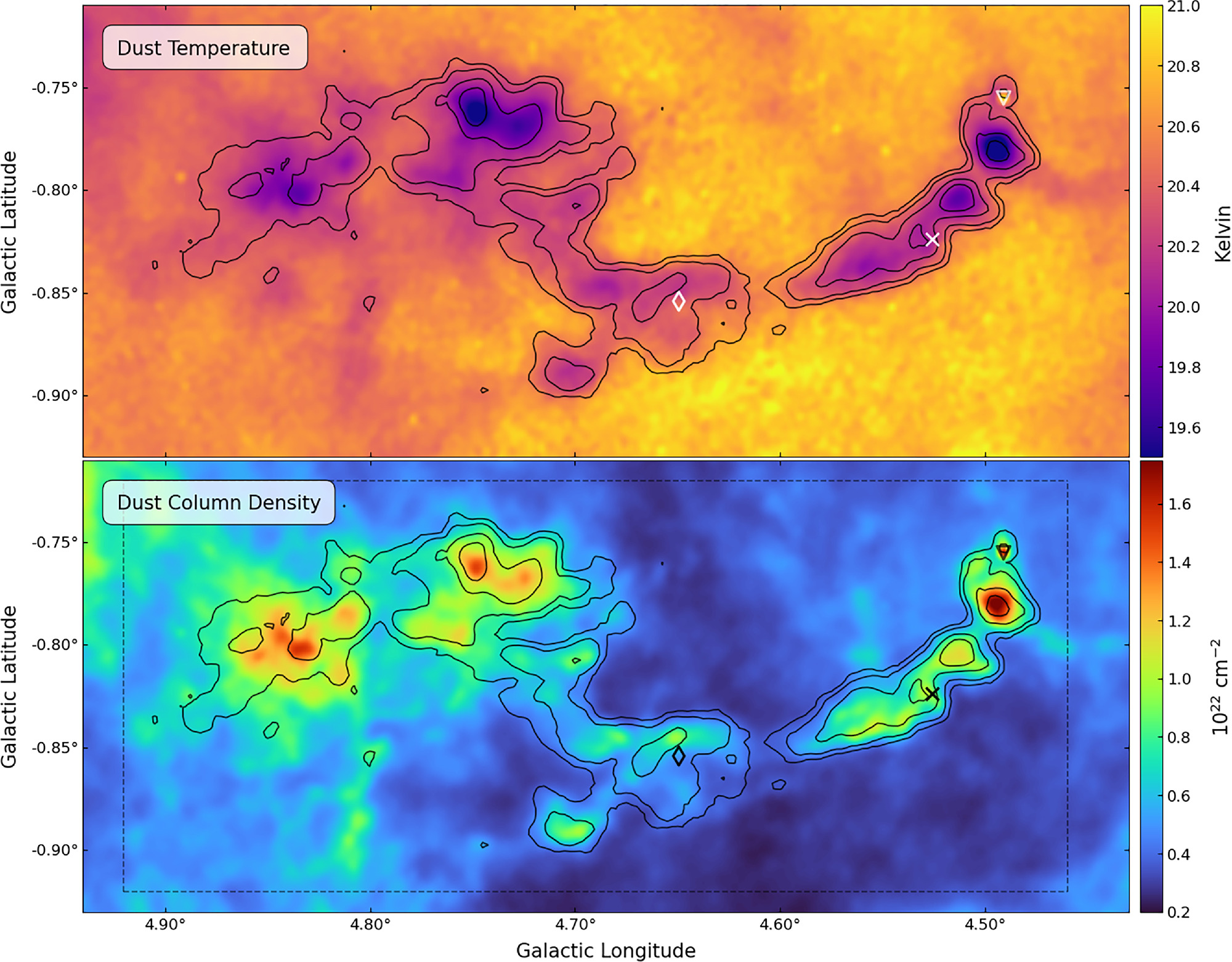
Figure 11. Dust temperature (top) and column density (bottom) of the Midpoint cloud from the K. A. Marsh et al. (2017) PPMAP data set. Both images have a resolution of 12″ and a sensitivity of ∼0.1 K (top) and 6 × 1019 cm−2 (bottom). Contours show the maximum intensity NH3 (1,1) emission at 0.15, 0.25, 0.5, and 0.75 K (see Figure 2). The × symbol shows the locations of the NH3 (3,3) maser from Section 3.2.2. The triangle marks the location of the 70 μm point source discussed in Section 5.3.2. The diamond shows the location of the radio point source discussed in Section 5.3.3. The gray dashed box, in the bottom panel, illustrates the region used to calculate the cloud mass—utilizing the column density data shown here.
Download figure:
Standard image High-resolution imageThe colder dust temperatures in the cloud (i.e., <20 K) are strongly correlated with the bright NH3 (1,1) regions, located in the innermost regions of the clumps and knots. The coldest of these is Knot D, with a measured dust temperature of 19.2 K. Knot E is observed to be hotter than all other NH3 peaks, with a temperature of 21 K. We note a slight positional offset between this hot dust core and the NH3 (1,1) peak of ∼10″. This offset is smaller than our GBT beam size (35″) and therefore could be caused by a pointing offset rather than a physical offset of the source. The emission surrounding Knot E appears to be slightly cooler (20.1 K) than the background emission (20.8 K), indicating this hot dust core could be embedded in a cooler envelope. We investigate this source, and the implication of an embedded core, in more detail in Section 5.3.2.
The N(H2) column density in the cloud is around 0.5–2.0 × 1022 cm−2 (Figure 11, bottom). The highest column densities in the region trace the NH3 emission morphology of M4.7–0.8. All of the knots located in the Filament show higher column densities in their interiors than the surrounding regions, with the highest column densities in M4.7–0.8 (1.82 × 1022 cm−2) associated with Knot D. Knot E also shows relatively high column densities (1.65 × 1022 cm−2), indicating that in addition to being quite compact (<10″; 0.4 pc), it is quite dense as well. We also note that these column density values are consistent with those in giant molecular clouds (GMCs; see Section 5.2).
The Nexus region of the cloud also shows moderately high column densities, with values around 1.0 × 1022 cm−2. There are two main high column density clumps in this region, the Main Clump (as annotated in Figure 2) and a secondary clump located in the Eastern region of the cloud (l = 4 84, b = −0
 80). This Eastern source does not appear to stand out in the NH3 emission nor the HC5N emission. However, this region does appear to be relatively bright in the 250 μm emission and in the Herschel short wavelength data sets (70 and 160 μm). This region of the cloud also appears to be quite large, extending well past the NH3 (1,1) contours and appearing to correlate with the IR-dark region around the Nexus, observed in the Spitzer 8 μm data (Figure 9, bottom).
The Gap region in the Filament also exhibits relatively low column density, with only a faint bridge connecting the eastern and western sides of the Filament. The low column density regime appears to be associated with a large cavity that extends toward the south, below the filament, and carves a lower-density region north, above the Gap. This lower column density at the location of the Gap could be an indication that feature is produced by nearby stellar feedback that has disrupted the Filament (e.g., C.-P. Zhang et al. 2016; X. Chen et al. 2023).
5. Discussion
In the following sections, we discuss the physical properties of the M4.7–0.8 cloud and the implications of our results from the previous section.
5.1. 3D Location of the Midpoint
Figure 12 shows the top-down geometry of the Milky Way Galactic Bar Dust Lanes from M. C. Sormani & A. T. Barnes (2019; see their Figure 2). The orientation and extent of the Galactic Bar Dust Lanes is marked with a dashed ellipse, with red and blue lines illustrating the near- and far-side Dust Lanes, respectively. The Galactic Bar Dust Lanes can roughly be divided into four main quadrants, labeled as Q1–Q4 in Figure 12. Quadrants 1 and 3 correspond to the near-side and far-side Dust Lanes, respectively. Quadrants 2 and 4 correspond to gas and dust that have “overshot” the GC (i.e., “spray”; T. Kim et al. 2024; see their Figure 1), from Quadrants 1 and 3, respectively, and are continuing to traverse the Bar. The gas and dust in these overshot regions can then interact with the approaching material on the opposing side to produce strong shocks from cloud–cloud collisions (M. C. Sormani et al. 2018a; M. C. Sormani 2021; S. R. Gramze et al. 2023). These shocks are visible as vertical features in position–velocity space (see Figure 1(b) and M. C. Sormani 2021).
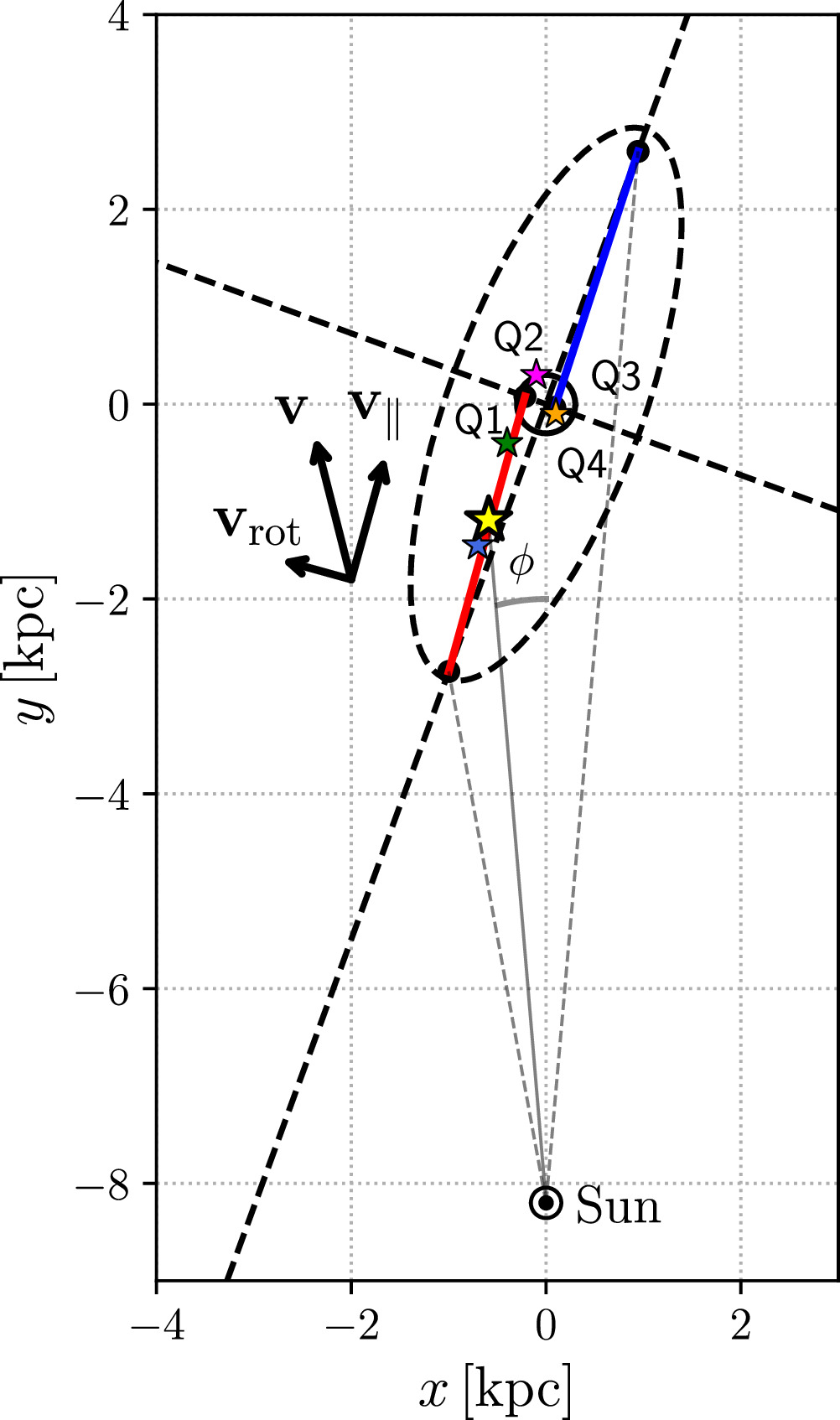
Figure 12. Top-down geometry of the Milky Way Galactic Bar Dust Lanes from M. C. Sormani & A. T. Barnes (2019; see their Figure 2). Here, the red and blue lines show the near-side and far-side Dust Lanes, respectively, matching the orientation shown in Figure 1(a). The yellow star shows the location of the midpoint cloud in this diagram at (−0.59, −1.19). Labeled are four quadrants of the Galactic Bar: Q1–Q4. Quadrant 1 (Q1) corresponds to gas and dust on the near side of the Galactic Bar Dust Lanes that is accreting into the Galactic Center (GC). Quadrant 2 (Q2) corresponds to matter from Q1 that has “overshot” the GC. Quadrant 3 (Q3) corresponds to the far-side Galactic Bar Dust Lanes that is accreting into the GC. Lastly, Quadrant 4 (Q4) corresponds to gas and dust that has “overshot” the GC from the far-side Dust Lane. ϕ shows an angle of 4 8, corresponding to the Galactic longitude of the cloud. The solid gray line shows the distance to the midpoint cloud at 7.035 kpc (yellow star; centered at x = −0.59, y = −1.19), while the dashed gray lines show the angular extent of the dust lanes (Figure 1(a)). The additional stars show the relative locations of G5 (blue), Bania’s clump (green), the Helix stream (pink), and Sgr E (orange).
Download figure:
Standard image High-resolution imageThe midpoint cloud is located at a Galactic longitude of roughly l ∼ 5° (angle ϕ in Figure 12). Based on the geometry shown in Figure 12, this suggests the cloud is located at (−0.59, −1.19), as marked by the yellow star. At this location, the cloud is calculated to be at a distance 7.035 kpc from the Sun. We also note the significantly low Galactic latitude of the cloud (b = −0 85), which suggests the cloud is below the midplane of the Milky Way. Using the geometry presented in A. A. Goodman et al. (2014; see their Figure 2), we calculate that M4.7–0.8 is located at 118.5 pc below the Sun, or 93.5 pc below the midplane (assuming the cloud has a distance of 7.0 kpc and the Sun has a positive z-height of 25 pc).
The cloud is also likely to be on the leading edge of the Dust Lanes. Orbital motions within the bar can create a shearing effect on the interstellar medium (ISM; E. Athanassoula 1992; E. Emsellem et al. 2015; F. Renaud et al. 2015). This strong shear can inhibit the formation of dense structures, such as clouds, which leads to low star formation within the bar, even in regions with relatively high densities. However, at the bar’s leading edge, supersonic turbulence, along with reduced shear and weaker tidal forces compared to the inner regions, promotes the formation and persistence of high-density structures (F. Renaud et al. 2015). The leading edges of the bar can also produce converging flows and large-scale shocks that promote the accumulation of dense gas into kiloparsec-scale structures (e.g., E. Athanassoula 1992).
5.1.1. Relative Location to Other Dust Lane Clouds
The connection between M4.7–0.8 and the Galactic Bar dust lanes, as indicated by the line-of-sight velocity, implies this cloud is part of a much larger structure of gas and dust. Part of this larger structure, in the region surrounding M4.7–0.8, is shown in Figure 1(c)—as highlighted by the 12CO contours. The Nexus region of the midpoint is located at a concentration of CO-rich gas and dust, with filamentary extensions toward the northeast, south, and west directions (see Figure 1(c)). The western filamentary extension, which we have labeled as the Filament, is the narrowest, and brightest, of these three in the 250 μm dust continuum. The southern and northeastern extensions appear to follow a larger, ∼20–30 pc wide, diffuse feature—as traced by 12CO emission. While the Filament may be too narrow to be resolved by the T. M. Dame et al. (2001) data set, southwest of the Filament is a large-scale structure in the dust continuum that appears to be traced by 12CO emission. The orientation of the Filament is similar to that of this western bridge, although follow-up spectral line observations of this region are necessary to confirm this possible association.24
Our observations of the Nexus reveal that the region contains numerous diffuse structures distributed throughout the region (Figure 2). Additionally, most of the dense gas in this region is located along the northern edge of the 12CO emission (see Figures 1(c)). However, we note that this offset could be the result of the low-resolution of the 12CO (0 125 pixel resolution). Follow-up observations of 12CO are necessary to confirm whether there is an offset between the 12CO and the dense gas, as traced by NH3.
Slightly “upstream” from the midpoint is the G5 complex (M5.4–0.4; N. J. Rodríguez-Fernández 2006; S. R. Gramze et al. 2023; A. Nilipour et al. 2024). G5 is suggested to be the result of a cloud–cloud collision (S. R. Gramze et al. 2023; see their Figure 15) from “spray” in Q4 that has overshot the CMZ and is colliding with accreting material in Q1 (see Figure 12). This results in the broad linewidths (i.e., “vertical feature”) observed in Figure 1(b) at l = 5 5 (N. J. Rodríguez-Fernández 2006; M. C. Sormani 2021). The 3D location of G5 is shown as a light-blue star in Figure 12. The location of the midpoint “downstream” from G5, in the direction of accretion, suggests M4.7–0.8 maybe the result of a prior interaction. If the locations of the “spray” are relatively constant, over a few Myr, the accretion time to traverse between the G5 and M4.7–0.8 locations, then M4.7–0.8 could be the result of a G5-like collision that has relaxed into a filamentary structure.
Further “downstream” from the midpoint, on the near-side Galactic Bar Dust Lane, is Bania’s clump (l = 3°; green star) and the Q1/Q2 transition (i.e., the x1 (Bar) and x2 (CMZ) intersection). The intersection of the CMZ and Bar are suggested to undergo strong shocks from cloud–cloud collisions (L. D. Anderson et al. 2020). Sgr E (orange star; Figure 12) is also suggested to be at the intersection between the x1 and x2 orbits and is argued to be undergoing intense star formation (L. D. Anderson et al. 2020). However, only ∼30% (0.8 M⊙ yr−1) of the mass is suggested to accrete into the CMZ (H. P. Hatchfield et al. 2021), indicating that a majority of the material overshoots the GC. The Helix stream is thought to be one of these regions (V. S. Veena et al. 2024; see the pink star in Figure 12). The Helix stream is argued to be associated with material that has overshot the CMZ from the near-side Dust lane and is continuing to traverse the Bar (V. S. Veena et al. 2024). The central velocities of this structure are quite high (100–200 km s−1), indicating that they are not likely associated with the x2 orbit.
5.2. Is M4.7–0.8 a GMC?
The leading edge of the Galactic Bar dust lanes tends to accumulate dense gas and promote the formation of overdense structures (E. Athanassoula 1992; F. Renaud et al. 2015). These overdense structures have the potential to form GMCs within the larger Dust Lane. The physical extent of the M4.7–0.8 cloud (∼60 pc) suggests this structure is likely a GMC within the leading edge of the near-side Dust Lane. GMCs are typically long (∼50–100 pc), dense (≳100 cm−3), massive (104–106 M⊙) clouds, often observed to be stellar nurseries (see M. Chevance et al. 2023, for a review of GMCs).
The observed length of the M4.7–0.8 cloud is consistent with many other GMCs observed in the Milky Way and other local GMCs in nearby galaxies (e.g., M. Chevance et al. 2023). These local GMCs tend to be filamentary in nature and have been argued to be the “bones” of the Milky Way spiral arms (e.g., A. A. Goodman et al. 2014; C. Zucker et al. 2015). Many of these GMCs also tend to have localized regions of higher densities (i.e., knots) where the gas has been concentrated by its self gravity. The M4.7–0.8 cloud also shows these types of localized knots that are observed in the Filament (Knots A–E).
In general, the N(H2) column densities in M4.7–0.8 (∼1022 cm−2; Figure 11, bottom) are similar to column density values measured in Disk GMCs (e.g., K. A. Marsh et al. 2017). However, when comparing our measured column density to values found in CMZ clouds, we find that CMZ clouds are an order of magnitude higher than those observed in M4.7–0.8 (∼1023 cm−2; C. Battersby et al. 2020). This suggests that the column density in the cloud will either likely increase during accretion into the CMZ or will coalesce with other clouds in the CMZ to result in the higher values observed in the inner region.
Using the column density data from K. A. Marsh et al. (2017), shown in Figure 11 (bottom), we can calculate a total mass for the M4.7–0.8 GMC. We used the PPMAP-MASS jupyter notebook, which calculates a cloud mass from the K. A. Marsh et al. (2017) column density data set (S. R. Gramze et al. 2023).25 This notebook first calculates an average column density over a specified region, which, in our case, uses the gray dashed box in Figure 11 (bottom). Using this average column density and area, with a set distance of 7.0 kpc (as calculated in Section 5.1), we estimate a cloud mass of 1.6 × 10⁵ M⊙. We note, however, that this cloud mass is lower than previous mass estimates calculated using the T. M. Dame et al. (2001) CO data set (M. C. Sormani & A. T. Barnes 2019).
M. C. Sormani & A. T. Barnes (2019) calculated a mass estimate of this region of roughly 105–106 M⊙ and used an XCO factor of 2 × 10²⁰(N(H2) cm−2)/(W(l, b) K km s−1) for their mass estimates (see their Figure 3). While this XCO factor, used in M. C. Sormani & A. T. Barnes (2019), represents the Galactic average, it is relatively high for CMZ clouds (A. D. Bolatto et al. 2013). Extragalactic studies of the CO-to-H2 conversion factor illustrate that this value tends to be lower in the inner region of galaxies when compared to the disk (e.g., Y.-H. Teng et al. 2023; I.-D. Chiang et al. 2024).
In the S. R. Gramze et al. (2023) mass calculation of the G5 GMC, they calculated a mass of 2 × 10⁵ M⊙—using an XCO factor of 1.5 × 1019 cm−2. However, in their PPMAP calculation, they are measuring a mass of 2 × 10⁴ M⊙. This order-of-magnitude increase in the XCO calculation, when compared with the PPMAP estimate, is similar to what we are observing in M4.7–0.8. This could be an indication that the XCO factor could be different from values used in the Disk and CMZ. Despite the range of mass estimates for this cloud (105–106 M⊙), which could be constrained in later publications, the estimated cloud mass falls well within the range for GMCs (104–106 M⊙; e.g., M. Chevance et al. 2023)—supporting our argument that M4.7–0.8 is a GMC.
Based on the large-scale velocity gradient of the near-side of the Galactic Bar Dust Lanes, shown in Figure 1(b), we would expect an increasing velocity gradient from east to west across the cloud of ∼+0.25 km s−1 pc−1. However, we instead observe a decreasing velocity gradient of −0.25 km s−1 pc−1 (see Section 3.2.1). We note that this is an average across the entire length of the GMC—where local velocity gradients in the Filament could be an order of magnitude higher (see Figure B2). This difference in the averaged velocity gradient across the cloud and the large-scale velocity gradient of the dust lanes could be an indication of some internal dynamics affecting the velocity structure of the GMC.
Velocity gradients across GMCs is not uncommon—as observed in E. Rosolowsky et al. (2003), who investigated the kinematics of 45 GMCs in M33 at 20 pc resolution (which would correspond to roughly 3 pixels beams−1 across M4.7–0.8). They observed, both positive and negative, velocity gradients across the GMCs in their sample that tend to be around 0.1 km s−1 pc−1 (see their Figure 7)—indicating that our measure velocity gradient across the entire GMC is slightly more extreme than their average. In 40% of their sample GMCs, E. Rosolowsky et al. (2003) saw counterrotation when compared with the disk rotation of M33. If M4.7–0.8 is the result of a previous cloud–cloud collision, as hypothesized in our previous section, then the resulting material could “decelerate,” resulting in this apparent counterrotation, as has been observed in previous simulations (R. G. Tress et al. 2020; see their Figure 16). Follow-up CO observations at <30″ resolution are needed to determine the kinematics of the extended region to ascertain whether the Filament is showing counterrotation relative to the bulk emission in the GMC. For this publication, we will limit our analysis to investigating the cloud kinematics and turbulence by using the spectral fitting information from Table 2 in the following section.
5.2.1. Elevated Turbulence in M4.7–0.8 When Compared to GMCs in the Disk
The CMZ is observed to have broader linewidths than the Galactic disk on similar size scales (e.g., R. Shetty et al. 2012). These broad lines are typically an order of magnitude greater than values measured in the disk. This increase is often attributed to turbulence; however, other possible scenarios include tidal shearing and feedback (e.g., J. D. Henshaw et al. 2023; see their Table 2). One method of understanding this turbulence is by plotting the measured linewidth against the physical radius of the region used to extract the line, also known as a Larson relationship (R. B. Larson 1981), defined as:

(see their Equation (1)). Here σ is the velocity dispersion in kilometers per second, and R is the radius of the cloud.
In Figure 13, we plot the R. B. Larson (1981) relationship for the cloud using the five spectra shown in Table 2 (shown as red “×” symbols) against other clouds in the CMZ (squares; T. Oka et al. 2001; J. Kauffmann et al. 2017; green and blue data points, respectively) and Galactic Disk GMCs (orange diamonds; M. Heyer et al. 2009). Data for these other clouds was pulled from J. S. Urquhart et al. (2015), who used NH3 (1,1) and (2,2) observations to target high-mass star-forming clumps in the Disk, shown as purple triangles. We also show data from V. S. Veena et al. (2024), who targeted the Helix stream (pink star in Figure 12) as light-pink circles. We note that NH3 (1,1) GBT observations of Sgr E exist (L. D. Anderson et al. 2020); however, these are single pointing spectra, and therefore, no radii information is available for this data set. We note, however, that the spectra were fit, and the measured values for Sgr E range from 1.3–40.3 km s−1.
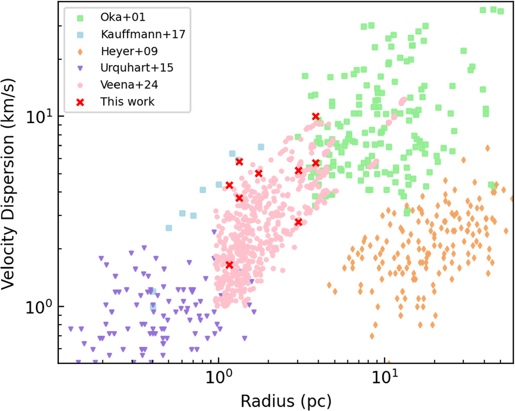
Figure 13. Larson linewidth–size relationship for the five regions shown in Figure 2 (marked as red × symbols here) compared with other survey data sets as labeled in the top-left legend. The velocity dispersion is measured from the spectral line fits shown in Figure 5. The values for the velocity dispersion and the radius are reported in Table 2. The green and blue squares show the GC data points from T. Oka et al. (2001) and J. Kauffmann et al. (2017), respectively. The orange diamonds show the Disk clouds from M. Heyer et al. (2009). The pink circles show the measurements from V. S. Veena et al. (2024), which is suggested to be downstream from the midpoint cloud. The purple triangles show the measured NH3 (1,1) linewidths of high-mass star-forming regions in the Disk (J. S. Urquhart et al. 2015).
Download figure:
Standard image High-resolution imageWe find that the measured velocity dispersion for the M4.7–0.8 cloud is fairly similar to values observed in the CMZ (green and blue squares), the Helix stream (pink circles), and high-mass star-forming regions (purple triangles) when compared with the Disk GMCs (orange diamonds). This similarity between the CMZ and Galactic Bar data points could be an indication that the turbulence observed in the CMZ is the result of infall to the gravitational potential. We note that the values measured in the midpoint cloud are fairly similar to those observed in the Helix stream (V. S. Veena et al. 2024). The Helix stream is argued to be “downstream” from the Midpoint and associated with material that has overshot the CMZ—indicating that it is likely located in Quadrant 2 (Figure 12). We note that this region is also “downstream” in the dust lanes from an “interaction location” (S. R. Gramze et al. 2023). Thus, the observed turbulence could be the result of a previous cloud–cloud collision. Results from M. Heyer et al. (2009) in Figure 13 represent GMCs in the Galactic Disk. Here we see that these GMCs have significantly lower velocity dispersions, while also presenting larger physical sizes, in comparison to our data and the results of V. S. Veena et al. (2024). This is not unexpected, due to the large (>10 pc) scale of the M. Heyer et al. (2009) sources. However, this is useful as a contrast. Further analysis of the structure of M4.7–0.8, with a focus on comparing cloud and clump properties to previously identified samples is beyond the scope of the current work and is planned for a follow-up investigation (L. K. Morgan et al. 2025, in preparation).
The higher linewidths observed in M4.7–0.8 are also consistent with the detection of the HC5N (9–8) transition. M. Chevance et al. (2023), and references within, noted that clouds that are rich, with complex molecules often displaying broader linewidths when compared with other clouds in the ISM. The detection of the HC5N (9–8) transition could be an indication that M4.7–0.8 is rich in other complex molecules, similar to other broad-line regions like the CMZ. Follow-up observations of additional complex molecules are currently underway with Atacama Large Millimeter/submillimeter Array (ALMA) to address this theory (N. Butterfield et al. 2025, in preparation).
5.3. Evidence of Star Formation at the Midpoint
Understanding star formation in barred spiral galaxies has been gaining momentum in recent years with the onset of high-resolution, high-sensitivity telescopes like ALMA and JWST (e.g., A. C. Phillips 1996; M. W. Regan et al. 1999; J. Neumann et al. 2019; K. Sheth et al. 2000; S. Verley et al. 2007; F. Renaud et al. 2015; A. Fraser-McKelvie et al. 2020; F. Maeda et al. 2023; L. Neumann et al. 2024). Bars within spiral galaxies are observed to contain abundant molecular material, which could potentially form stars (S. Díaz-García et al. 2021). This region of the galaxy also has a higher stellar density and is more metal-rich than the disk at similar radii (J. Neumann et al. 2024). These extragalactic studies of barred galaxies found that primarily low-mass galaxies host star formation in their bars and are typically usually on the leading edge of the bar (A. Fraser-McKelvie et al. 2020). Furthermore, these sites of star formation are regulated by shear forces, turbulence, and gas flows (F. Renaud et al. 2015; A. Fraser-McKelvie et al. 2020). In this section, we explore possible signs of star formation in the cloud by focusing on Knots B (Section 5.3.1) and E (Section 5.3.2) and investigate possible stellar feedback producing the Shell (Section 5.3.3).
5.3.1. Is There Star Formation in Knot B?
Knot B is observed to contain several tracers of possible star formation, including the new detection of an NH3 (3,3) maser (Section 3.2.2). Analysis of the dust continuum emission shows compact emission southwest of the (3,3) maser, near the observed edge of the knot, in the 8, 12, 24, 70, and 870 μm bands (red box in Figures 8–10). Figure 14 shows a higher-resolution image of the 8 μm data in this compact emission. Overlaid are contours showing emission at 870 μm (blue; Figure 8), 70 μm (yellow; Figure 9, bottom), and 24 μm (red; Figure 10, top).
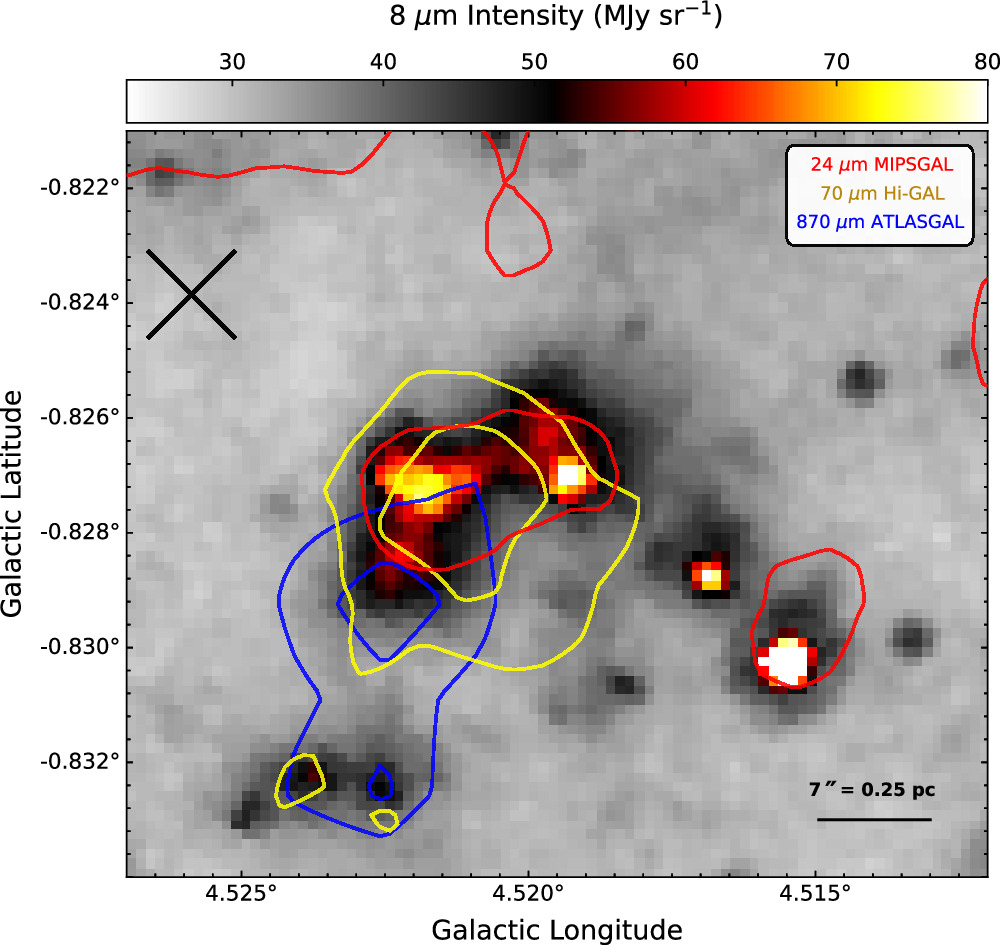
Figure 14. Shown here is 8 μm emission of the extended source located near the head of Knot B (red box in Figures 8–10). The blue contours trace the ATLASGAL 870 μm emission, from Figure 8, at 0.6 and 0.68 Jy beam−1. The yellow contours trace the Herschel 70 μm emission, from Figure 9, at 0.032 and 0.04 Jy pixel−1. The red contours trace the MIPSGAL 24 μm emission, from Figure 10, at 20.5 MJy sr−1. The black × symbol shows the central location of the NH3 (3,3) maser (Section 3.2.2). A scale bar of the region is shown in the bottom-right corner, assuming a distance of 7.0 kpc.
Download figure:
Standard image High-resolution imageThe 8 μm observations show this source is extended (∼0.5 pc) and contains several bright point sources. The 24 μm emission is closely associated with the bright emission observed in the 8 μm. The 70 μm emission is concentrated toward the bright, extended 8 μm structure near the center of the region. The 870 μm emission appears to be marginally offset from this central source and slightly elongated—extending away from the main concentration of mid-IR emission.
The detection of relatively compact emission at mid-IR (8, 12, 24, and 70 μm) and in the submillimeter (870 μm), with no compact emission detected at far-IR wavelengths (160 and 250 μm), could indicate that this source is an H ii region. The detection in the 8, 12, 24, and 70 μm bands is likely associated with the hot dust component. The compact emission observed in the 870 μm band could be associated with the tail end of the “free–free” Bremsstrahlung emission from radio and millimeter wavelengths. Both of these emission mechanisms, free–free emission at submillimeter and hot dust at the mid-IR, are observed to be associated with H ii regions (e.g., C. G. Wynn-Williams 1974).
Furthermore, the detection of an NH3 (3,3) maser may also support this argument of possible star formation in Knot B. NH3 (3,3) masers have been previously observed toward regions of high-mass star formation (e.g., K. E. Kraemer & J. M. Jackson 1995; Q. Zhang & P. T. P. Ho 1995). K. E. Kraemer & J. M. Jackson (1995) observed NH3 (3,3) masers near the ends of high-velocity molecular outflows as the results of shocks. The slight offset in the maser location could be due to the jets, from the massive star formation complex, interacting with the bulk emission in the filament.
While the mid-IR and submillimeter observations, combined with the maser detection, support this argument for an H ii region, we note that the source is lacking radio counterparts. We investigated the 2–3 GHz VLASS 3.0 data set (M. Lacy et al. 2020) for radio counterparts in the region and none were found above a 3σ level (<0.4 mJy beam−1). The GLOSTAR C-band (6 GHz) survey was also checked, and no detection was found above a 3σ level in the B-configuration data of this survey either (<0.3 mJy beam−1; A. Y. Yang et al. 2023). This nondetection at low radio frequencies could indicate that the turnover for the free–free emission in the radio spectrum is above this frequency range, or the emission is below the noise floor in the VLASS and GLOSTAR surveys. High-resolution radio and millimeter observations of this source are needed to determine (1) if this is indeed an H ii region by investigating the spectral energy distribution (SED) of the source, and (2) if the velocity of source is consistent with the GBT molecular emission, thereby confirming the association with the cloud.
5.3.2. Is Knot E a Free-floating Evaporating Gas Globule?
Free-floating evaporating gas globules (frEGGs) are small, dense, isolated dark clouds of gas and dust that are being eroded by nearby radiation (e.g., R. Sahai et al. 2012b,a; N. J. Wright et al. 2012). These sources tend to have a tadpole- or cometary-like structure, containing a bright head and a fainter extended envelope (e.g., B. Lefloch & B. Lazareff 1994; B. Lefloch et al. 1997; R. Sahai et al. 2012a). This fainter envelope is produced by the erosion of the globule by radiation, indicating the direction of the “tail” is oriented away from the ionizing source (F. Bertoldi & C. F. McKee 1990; N. J. Wright et al. 2012). These cometary globules are argued to form under the effects of radiative-driven implosion scenarios (e.g., F. Bertoldi & C. F. McKee 1990). The size of these frEGGs can be much larger (20,000–110,000 au; 0.1–0.5 pc) than their proplyd counterparts found in Orion (40–350 au; W. J. Henney & C. R. O’Dell 1999; N. J. Wright et al. 2012), as the size of the eroding source can depend on the distance to the ionizing source of radiation.
Knot E shows many characteristics that are in agreement with traits found in frEGGs. Located at the tail end of the Filament (see Figure 2), Knot E appears to be distinctly separated in both position and velocity from the neighboring Knot D and the rest of the Filament. Knot E is also observed to be relatively dense (N(H2) ∼1.5 × 1022 cm−2) and compact (d < 1 pc), suggesting the source is more similar to frEGGs than the proplyds found in Orion. Knot E also appears to be cometary in the dust continuum, containing a compact core with diffuse emission extended north of the compact source. This cometary structure is best observed in the three-color image (Figure D1), which shows a composite of the three Herschel bands from Figure 9. The orientation of the cometary tail, nearly directly north when viewed in Galactic coordinates, would suggest the source producing the radiation is located south of Knot E, and could possibly be associated with Knot D. We note that the direction of the tail is also perpendicular to the direction of accretion; therefore, the cometary morphology is not likely the result of the cloud’s movement through the Bar. The extended envelope is observed to be mid-IR dark, showing extinction in the 8–24 μm data, while the compact emission is observed to be mid-IR bright, showing bright compact emission in the 8–24 μm data set (Figure 10). B. Lefloch et al. (1997) saw a similar morphology in several cometary globules in IC 1848—which showed a bright head and dark tail.
The mid- and far-IR compact emission in Knot E was previously investigated in Hi-GAL survey work conducted by D. Elia et al. (2017; their catalog source ID 1948; marked with a red triangle in Figures 8–10). D. Elia et al. (2017) calculated a mass of 11.12 M⊙ and a dust temperature of 14.59 K for the 70 μm point source. We note, however, that this value of the dust temperature measured in D. Elia et al. (2017) is significantly lower than the temperature measured in K. A. Marsh et al. (2017; 20.8 K; see Figure 11, top). This discrepancy in the temperature is could be caused by the cometary structure of the source, which could contain a hot object embedded in a cooler envelope. Another alternative could be the inclusion of bremsstrahlung (free–free) emission in the longer wavelengths. D. Elia et al. (2017) used 870 μm emission in their dust temperature calculations, when available. Figure 8 shows 870 μm emission is present in this region. If, however, this emission is associated with free–free emission rather than the tail end of the Planck distribution at the longest wavelengths, this could then inflate the emission values at the longest wavelengths, resulting in a lower temperature measurement. K. A. Marsh et al. (2017) calculated their temperatures and column densities using a PPMAP technique, which calculates a column density per temperature “slice.” Slice 6 (18.4015 K) and slice 7 (21.7373 K) show a structure most similar to the emission distribution shown in Figure 9, suggesting the dust temperature is likely within this range—similar to the values shown in Figure 11.
If Knot E is being eroded by a nearby massive star (as is necessary for a frEGG source), then one would expect to see evidence of radio emission from the winds of these massive stars and free–free emission in Knot E. As mentioned in Section 5.3.1, the VLASS and GLOSTAR survey were checked, and no radio emission was observed in the region above a 3σ level (<0.4 mJy beam−1). We note, however, that we may be sensitivity limited to detecting these massive stars. Roughly 20% of the X. Lu et al. (2019) sample of point sources in the GC were below this 3σ level (<0.4 mJy beam−1), with at least one showing a positive spectral index, indicating the radio emission is likely thermal (e.g., see their source C86). Thus, without sensitive radio continuum observations (X. Lu et al. 2019 reported a sensitivity of 0.025 mJy beam−1 in their low-rms fields), we are unable to determine whether there are massive stars in the region.
5.3.3. Is the Shell Evidence of Feedback?
Feedback from evolved massive stars can influence their surrounding material by injecting energy and momentum into the nearby gas and dust. Most of this ejected material is generally modeled to be isotropic, resulting in the formation of bubbles and shells in the ISM (e.g., R. Weaver et al. 1977; A. T. Barnes et al. 2023; E. J. Watkins et al. 2023).
We observe a shell-like feature in the M4.7–0.8 cloud that may be associated with feedback, labeled as the “Shell” (see Figure 2). The Shell shows a hollow morphology both in the maximum intensity images (Figure 2) and in the channel maps (Figure B3). This morphology is also observed in the dust continuum as well (see Figure 9). Furthermore, the hollow morphology is also faintly visible in the position–velocity diagram (Figure B2). These signatures are typically characteristic of a bubble-like morphology. Along the eastern side of the shell, we observe an increase in the emission. This region also corresponds to the region of the shell with the highest column density (Figure 11).
The 2–3 GHz VLASS catalog was checked for possible radio counterparts, and a point source was detected within the region denoted as the Shell: l = 4 6492524, b = −0
 8542642 (marked with a red diamond in Figure 9). A figure showing the VLASS point source is included in the Appendix (Figure C1). A cross-examination of the location of radio point source with the far- and mid-IR data sets indicates this source is lacking an IR counterpart. As the nature of this radio point source is unknown, as well as the velocity of the point source, it is unclear if this source is interacting with the cloud or if this is a chance alignment.
However, we note that the location of the radio point source is nearest to the edge of the Shell with the highest emission. If this radio feature was interacting with the Shell, then we could see an increase in emission nearest to this interaction location. However, from these single survey observations, this possible interaction is speculative, at best. Therefore, high-resolution follow-up study of this region at radio wavelengths is necessary to determine (1) the nature of this radio point source, (2) the line-of-sight distance to the source to determine if it is in the dust lanes, and (3) if this point source is interacting with (or possibly creating) the Shell feature observed in the Filament.
The nature of the Shell is also unclear. We investigated several SNR catalogs, and no SNRs have been discovered in the region near the midpoint. With no evidence found for an ionizing influence upon the observed region, the Green SNR catalog (D. A. Green 2019),26 the Chandra SNR Catalog,27 and the SNRCat (G. Ferrand & S. Safi-Harb 2012)28 were searched for previous observations that might support an SNR-driven scenario. Additionally, the ATNF pulsar catalog29 was also searched for any coincident pulsars that might indicate the presence of a prior supernova in the region. All searches returned no likely candidates that could be associated with a driving dynamical force in this region. Higher-resolution observations of the Shell are needed to disentangle the kinematics at this location and calculate the momentum and energy of the possible expansion. These calculations would then give insight on the energy needed to power the expansion and the possible mechanisms that could be driving the expansion.
6. Conclusion
We report the detection of a previously unknown GMC located at the midpoint of the near-side Galactic Bar Dust Lanes (M4.7–0.8). In this publication, we present 25 GHz radio observations of dense gas that is associated with material accreting into the GC. In these observations, taken with the GBT, we targeted the NH3 (1,1)–(4,4), and the HC5N (9–8) transitions. These single-dish observations observed the main “Nexus” and “Filament” of the GMC (0 5 × 0
5 × 0 25 area) with 31″ angular resolution (∼1 pc at a distance of 7.0 kpc to the cloud). A comparison with IR survey data shows a far-IR dust component that is well correlated with the NH3 emission (Section 4). In addition to this dense gas detection, we also report the following results:
- 1.3D Location in the Dust Lane. Based on the observed Galactic longitude (l ≃ 5°) and velocity (v ∼ 200 km s−1), we argue that M4.7–0.8 is located on the near-side Dust Lane (Section 5.1). We compare the location of M4.7–0.8 to the M. C. Sormani & A. T. Barnes (2019) toy model of the Dust Lanes and argue the cloud is located at a distance of 7.0 kpc (Figure 12). The negative Galactic latitude of the cloud (b = −0
 85) also indicates that it is about 93.5 pc below the Galactic midplane, using the geometrical model presented in A. A. Goodman et al. (2014).
 - 2.Properties of the GMC. The M4.7–0.8 GMC has a length of roughly 60 pc in Galactic longitude and a vertical extent of ∼20 pc in Galactic latitude (assuming a distance of 7.0 kpc). Utilizing the K. A. Marsh et al. (2017) PPMAP survey data (shown in Figure 11), we measure high column densities (∼1022 cm−2) and cold dust temperatures (∼20 K) in the GMC (Section 4.1). Using the column density data, and the PPMAP-MASS jupyter notebook, we calculate a cloud mass of 1.6 × 10⁵ M⊙ (Section 5.2). Based on the size, mass, and column density of M4.7–0.8, all of which are typical of the properties of Galactic GMCs, we argue that M4.7–0.8 is a GMC. We also make a comparison of the cloud’s linewidths (reported in Table 2) to clouds in the Disk and CMZ, using the Larson relationship, and find relatively broad linewidths in M4.7–0.8 (Section 5.2.1). These broader linewidths are similar to values reported in CMZ clouds, indicating that M4.7–0.8 has elevated turbulence compared to Disk clouds and GMCs.
- 3.New NH3 (3,3) Maser Detection. We detect a previously unknown NH3 (3,3) maser in our data set (Section 3.2.2). This new NH3 (3,3) maser is located in Knot B (see black × symbol in Figure 2). The spectral analysis of this maser shows it has a central velocity of 193.16 ± 0.01 km s−1 and a narrow linewidth of 0.37 ± 0.01 km s−1.
- 4.New Sites of Star Formation. We observe two new sites of possible star formation in the cloud: Knots B and E. Knot B contains the newly detect NH3 (3,3) maser—a common tracer of shocks from outflows. This region also contains extended 8 μm emission (Figure 14) that also has 24, 70, and 870 μm emission—known tracers of star formation (Section 5.3.1). This region shows a brightening in the 870 μm emission, when compared with the extended structure and the 250 μm emission, indicating that we may be detecting free–free emission from a possible H ii region. However, sensitive radio observations are needed to confirm this. The other source, Knot E, displays a cometary-like structure in the dust continuum that is extended at far-IR wavelengths and compact in mid/near-IR wavelengths. Knot E is dense, showing extinction in the 8 μm Spitzer data (Figure 10, bottom) and a high column density in the K. A. Marsh et al. (2017) PPMAP data (Figure 11, bottom). This region also shows a relatively high dust temperature (∼21 K) compared to the cooler envelope. We further investigate Knot E as a possible free-floating evaporating gas globule (frEGG; see Section 5.3.2).
- 5.Evidence of Feedback in the GMC. The M4.7–0.8 cloud also contains what appears to be a shell-like structure that we label as “the Shell” (see Figure 2). This structure contains a brighter rim in the NH3 emission, with a cavity toward its center (Section 3.1). A radio continuum point source is observed within the Shell, but its relation to the Shell is uncertain without additional observations (Section 5.3.3).

Acknowledgments
The collaboration would like to thank the GBT operators for their assistance with these observations. N.B. would also like to thank Dr. Ryan Boyden (UVA) for his helpful discussion on frEGGS. M.C.S. acknowledges financial support from the European Research Council under the ERC Starting Grant “GalFlow” (grant 101116226) and from Fondazione Cariplo under the grant ERC attrattività No. 2023-3014. C.B. and H.W. were supported by the NSF REU program at the National Radio Astronomy Observatory and the Green Bank Observatory. The authors would also like to thank the anonymous referee for providing help in strengthening this publication.
This research has made use of the CIRADA cutout service at URL cutouts.cirada.ca, operated by the Canadian Initiative for Radio Astronomy Data Analysis (CIRADA). CIRADA is funded by a grant from the Canada Foundation for Innovation 2017 Innovation Fund (Project 35999), as well as by the Provinces of Ontario, British Columbia, Alberta, Manitoba and Quebec, in collaboration with the National Research Council of Canada, the US National Radio Astronomy Observatory, and Australia’s Commonwealth Scientific and Industrial Research Organization.
This work is based in part on observations made with the Spitzer Space Telescope, which is operated by the Jet Propulsion Laboratory, California Institute of Technology under a contract with NASA. Herschel is an ESA space observatory with science instruments provided by European-led Principal Investigator consortia and with important participation from NASA. The Green Bank Observatory is a facility of the National Science Foundation operated under cooperative agreement by Associated Universities, Inc. This publication is based on data acquired with the Atacama Pathfinder Experiment (APEX) under the ATLASGAL large program (F. Schuller et al. 2009). APEX is a collaboration between the Max-Planck-Institut fur Radioastronomie, the European Southern Observatory, and the Onsala Space Observatory.
Software: CASA (International Consortium Of Scientists 2011), pyspeckit (A. Ginsburg et al. 2022), spectral-cube, astropy, pvextractor, Jupyter.
Appendix A: NH3 (5,5) Observations
In our DDT observations of the Filament, we included a spectral window centered on the NH3 (5,5) line as a test to determine whether higher transitions of NH3 were present in the cloud. This spectral window replaced the HC7N (21–20) transition, which was observed to be a nondetection in all previous observations. While we do not include this transition in our analysis, due to the incomplete coverage of the cloud, we show the detection here for future analysis of the Filament.
Figure A1 shows the maximum intensity emission in the NH3 (5,5) transition— similar to the plots shown in Figures 2 and 3. The NH3 (5,5) para-line emission closely follows the (4,4) para-line emission. Knots A–D are clearly visible, with Knot C being the brightest emission in this field. Similar to the (4,4) line, the knots are more elongated than what is observed in the lower NH3 transitions, and Knot E is not detected in the (5,5) data cube.
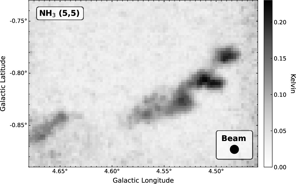
Figure A1. Peak antenna temperature for the NH3 (5,5) in the Filament. The beam size is shown in the bottom-right corner.
Download figure:
Standard image High-resolution imageAppendix B: Additional Kinematic Analysis
B.1. Moment 1 Map of the Filament
Figure B1 shows the Moment 1 map for the NH3 (3,3) emission in the Filament, constrained to the velocities in this region of the cloud (181–200 km s−1). The velocity gradients in the knots are slightly more prominent in this constrained velocity range.
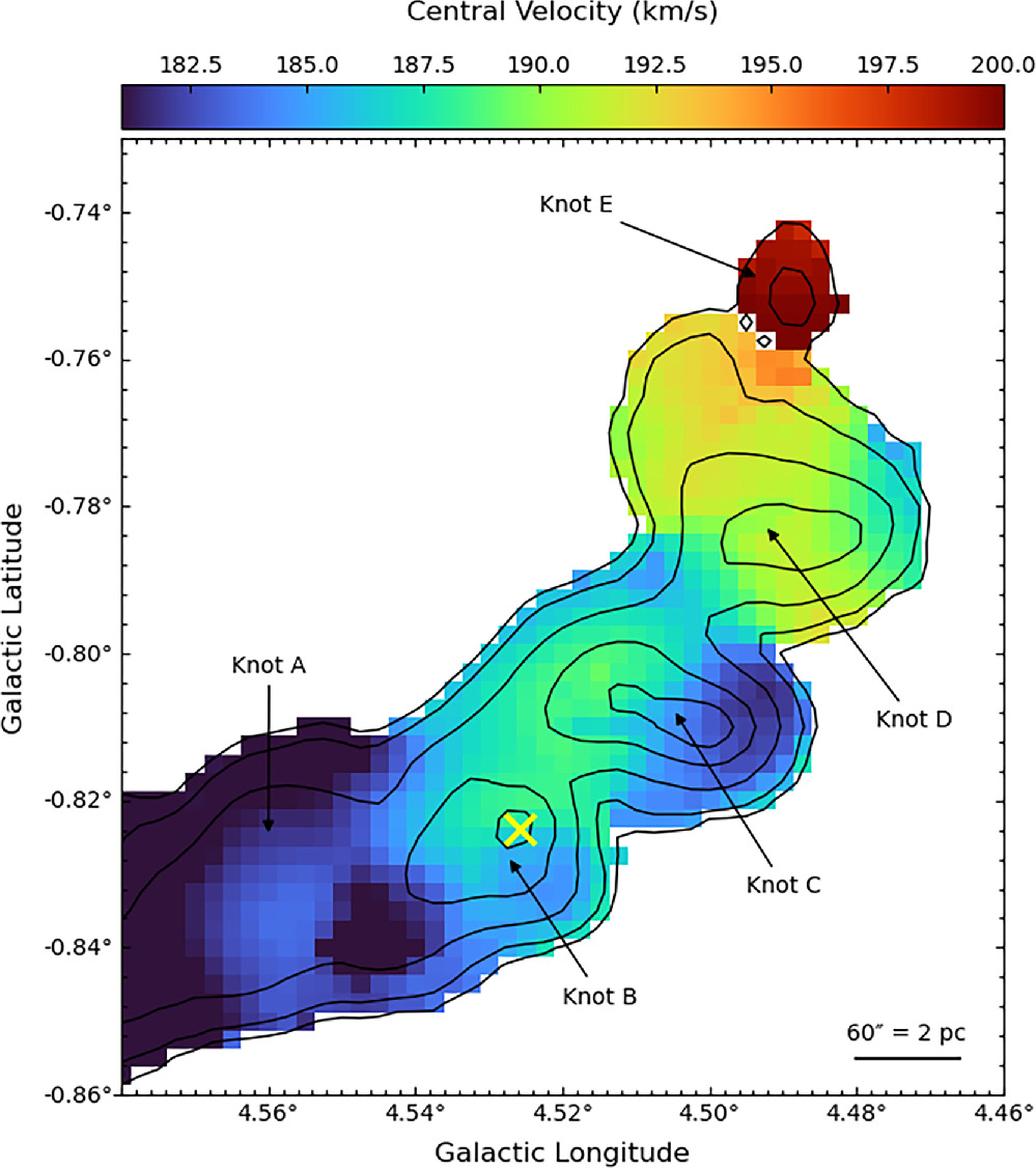
Figure B1. Central velocity (Moment 1) of the NH3 (3,3) emission in the Filament Knot’s A–E. This data, previously shown in Figure 6, is constrained both spatially and spectral to the region around the Filament. The location of the NH3 (3,3) maser, discussed in Section 3.2.2, is marked with a yellow “ × ” symbol.
Download figure:
Standard image High-resolution imageB.2. Position–Velocity Diagram
Figure B2 shows a position–velocity diagram for the M4.7–0.8 molecular cloud. This plot was made in python using pvextractor,30
with a slice width of 0 1625, centered at b = −0
 81, and covering a Galactic longitude from l = 4
 9 to 4
 46. Most of the emission in the cloud is between 170 and 220 km s−1 (solid black lines in Figure B2). The 230 km s−1 cloud, discussed in Section 3.2.1 and annotated in Figures 6 and B2, is observed to be a distinct feature in position–velocity space.
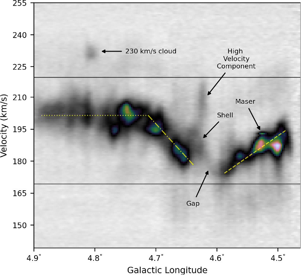
Figure B2. Position–velocity diagram of the NH3 (3,3) emission in M4.7–0.8 cloud from l = 4 9 to l = 4
 46, centered on b = −0
 81 with a width of 0
 1625. The horizontal black solid lines (at 170 and 220 km s−1) show the velocity range covered in the channel maps in Figure B3. There is a narrow velocity feature at l = 4
 52 that we are interpreting as maser emission. We discuss this feature in detail in Section 3.2.2. The yellow dashed and dotted lines show the velocity gradients.
Download figure:
Standard image High-resolution imageBetween l = 4 9 and l = 4
 7, the velocity in M4.7–0.8 is fairly constant—around 200 km s−1 (dotted yellow line). Most of this emission is associated with the region we are defining as the “Nexus.” At l = 4
 7, we observe a gradual decrease in the velocity from ∼200 to ∼ 180 km s−1 (dotted–dashed line). This Δv (∼20 km s−1) and Δl (∼0
 075, ∼10 pc) results in a velocity gradient of ∼2 km s−1 pc−1. Here, around l = 4
 6–4
6–4 65, we observe a gap in the structure, where the emission is relatively faint. This feature is associated with the “Gap” region annotated in Figures 2 and 6. At lower Galactic longitudes, we observe a second velocity gradient between 4
 6 and 4
 5, with velocity increasing from 170 at l = 4
 6 to 200 km s−1 at l = 4
 5 (dashed line), resulting in a velocity gradient of ∼2 km s−1 pc−1. Both of the nonzero velocity gradients are associated with the feature we are identifying as the “Filament.”
In addition to the “Gap” between the two velocity gradients, we also observe a feature at a higher velocity: 210 km s−1. This feature is associated with emission in the high-velocity component (as annotated in Figure 6, top), which shows high velocities and broad linewidths in that figure (middle and bottom panels, respectively). Lastly, we also observe a narrow velocity feature around l = 4 53 and v = 195 km s−1. We have marked this feature as possible maser emission in Figure B2, and will discuss this emission feature in more detail in Section 3.2.2. The hyperfine structure of the NH3 (3,3) line is also clearly visible in the Filament region of the cloud as faint emission that is ±20.7 and ±28.2 km s−1 from the main, bright peak.
B.3. Channel Maps
Figure B3 shows channels maps of the NH3 (3,3) emission, from 170–220 km s−1, for the M4.7–0.8 cloud. This velocity range contains all of the emission in M4.7–0.8, as observed in Figure B2, with the exception of the 230 km s−1 cloud and a portion of the high-velocity component. Each panel was made by integrating the emission over a Δv = 5 km s−1 velocity range, as specified in the bottom-left corner, essentially creating a Moment 0 map for each panel (Equation (1)).
The general, large-scale velocity gradient of 0.25 km s−1 pc−1, discussed in Section 3.2.1, is visible in this figure. Here, most of the higher-velocity emission (195–210 km s−1) is on the eastern side of the panels in the region associated with the Nexus. The lower-velocity emission (170–195 km s−1) is generally observed toward the western side of the panels in the region associated with the Filament. However, faint emission from the hyperfine lines is visible at ±20.7 km s−1 from the main emission features. In the 175–180 and 180–185 km s−1 panels, the Shell feature is quite prominent and shows an increase in brightness along the leftmost rim. The high-velocity component, discussed in Section 3.2.1, is also visible in this figure and is the brightest emission in the filament in the 200–215 km s−1 panels. The spatial location of the high-velocity component appears to coincide with an observed cavity visible in the 180–185 km s−1 panel.
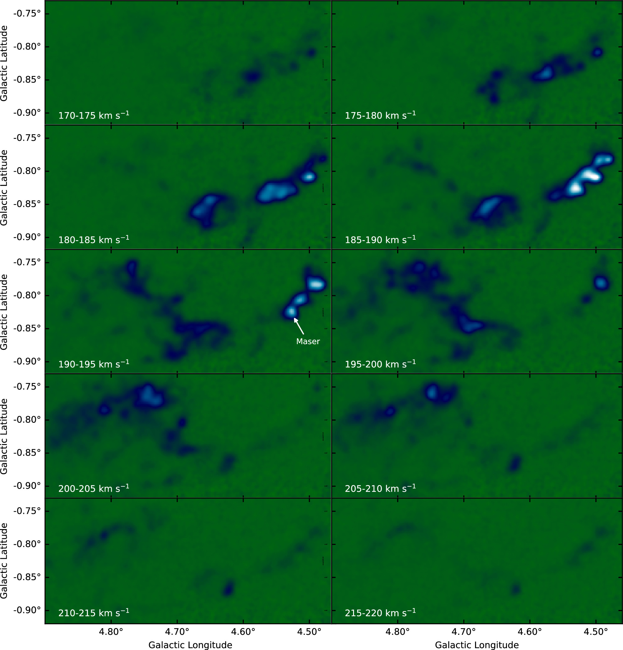
Figure B3. Integrated emission (moment 0) of the NH3 (3,3) line, binned by 5 km s−1, from 170–220 km s−1. The NH3 (3,3) maser location is marked in the 190–195 km s−1 channel. The noise floor is more prominent in the left side of each panel due to the lower time-on-source of the DDT observations.
Download figure:
Standard image High-resolution imageAppendix C: Radio Point Source
Figure C1 shows the radio point source detected in the vicinity of the Shell from the VLA Sky Survey (VLASS) data set (M. Lacy et al. 2020). This survey is an all sky survey at the S band (2–3 GHz) with 2″ resolution. Using this survey data, we detected a radio point source in the region denoted as “the Shell” (Section 3.1). The radio point source is detected at 1.95 mJy beam−1.
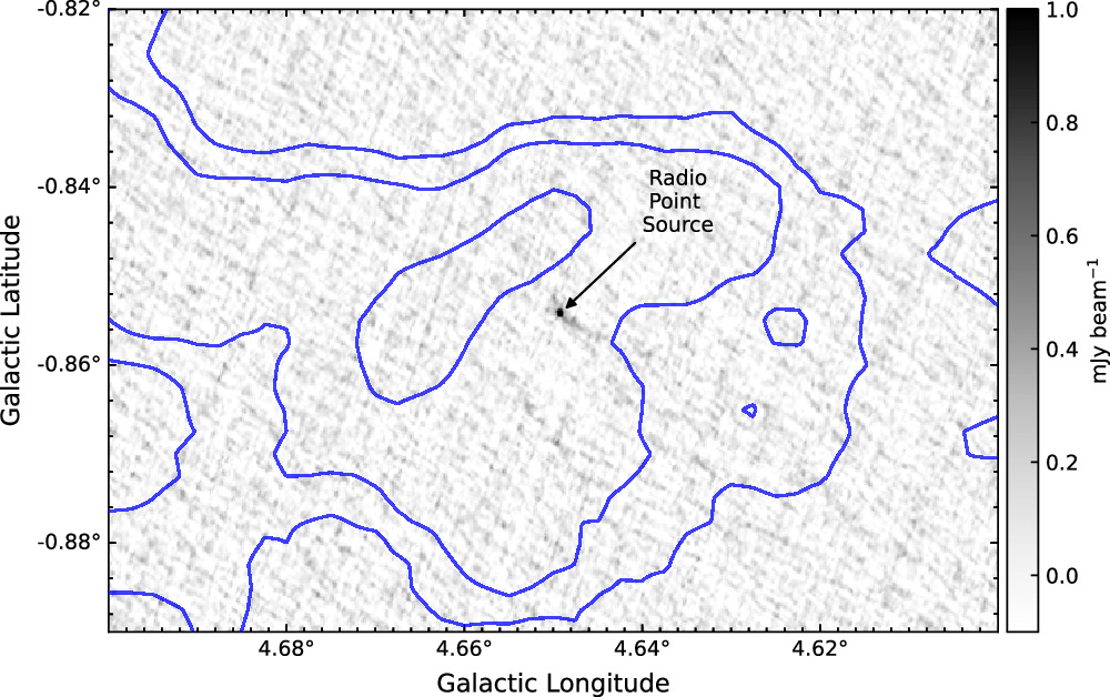
Figure C1. Shown here is 2–4 GHz radio emission from the VLASS data set showing the point-source detection toward the Shell (2 4, 120 μJy beam−1; M. Lacy et al. 2020). The blue contours show the NH3 (1,1) data at 0.15, 0.25, 0.50, and 0.75 K. While not shown, this point source is also detected in the 6 GHz GLOSTAR radio survey. This unresolved point source has a flux density of 1.95 mJy, assuming the source is unresolved in the VLASS data set.
Download figure:
Standard image High-resolution imageAppendix D: Three-color Dust Continuum
Figure D1 shows a three-color composite image of the Herschel bands shown in Figure 9, where 70 μm is blue, 160 μm is yellow, and 250 μm is red. The cometary structure of Knot E, discussed in Section 5.3.2, is visible in this three-color image.
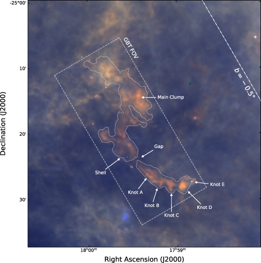
Figure D1. Three-color Herschel composite image of dust at the midpoint (M4.7–0.8) of the Galactic Bar Dust Lanes, showing PACS 70 μm (blue), PACS 160 μm (green), and SPIRE 250 μm (red). White contours show the 12CO emission associated with the Galactic Bar Dust Lanes (D. J. Marshall et al. 2008; M. C. Sormani & A. T. Barnes 2019). The dashed white box shows the FOV of the GBT observations (Figures 2, 3, and 6). The single contour traces the NH3 (1,1) peak antenna temperature at the 15σ level (150 mK; Figure 2, top). The dotted–dashed line shows b = −0 5.
5.
Download figure:
Standard image High-resolution imageFootnotes
- 12
https://greenbankobservatory.org/portal/policies/#publications. The National Radio Astronomy Observatory and Green Bank Observatory are facilities of the U.S. National Science Foundation operated under cooperative agreement by Associated Universities, Inc.
- 13
The NH3 (5,5) transition was not observed in the Nexus region.
- 14
The GBTIDL package can be found here: https://gbtidl.nrao.edu/.
- 15
The gbtgridder python program is available at https:// github.com/GreenBankObservatory/gbtgridder.
- 16
This issue was related to a deterioration in the telescope track foundation and has since been remedied (D. Frayer 2025, private communication).
- 17
The dataset presented in this publication is publicly available at https://www.gb.nrao.edu/GbtLegacyArchive/BARFLYS/Pilot_Study/Midpoint/.
- 18
- 19
A more detailed analysis on the clump structure in the cloud is underway and will be presented in a separate publication (L.K. Morgan et al. 2025, in preparation).
- 20
The SpectralCube python program is available at https://github.com/radio-astro-tools/spectral-cube.
- 21
The pyspeckit python program is available at https://github.com/pyspeckit/pyspeckit.
- 22
Figure B1 shows a scaled version of the moment 1 map for the knots associated with the Filament.
- 23
These data are publicly available: (http://www.astro.cardiff.ac.uk/research/ViaLactea/). M4.7–0.8 is located in field l004.
- 24
A follow-up program to study the entirety of the Dust Lanes using the GBT has been approved, for 200 hr, under the “Bar Ammonia Radiation in Lanes Filaments and YSOs Survey (BARFLYS; https://greenbankobservatory.org/science/gbt-surveys/barflys/)” large program, and will be carried out over the next 3 yr.
- 25
The jupyter notebook used to calculate the GMC mass from the K. A. Marsh et al. (2017) column density data set can be found here (https://github.com/SpacialTree/lactea-filament/blob/main/lactea-filament/notebooks/ppmap_mass.ipynb).
- 26
D. A. Green 2025, ‘A Catalogue of Galactic Supernova Remnants (2024 October version)’, Cavendish Laboratory, Cambridge, United Kingdom (available at https://www.mrao.cam.ac.uk/surveys/snrs/).
- 27
- 28
- 29
- 30
The pvextractor python program is available at https://github.com/radio-astro-tools/pvextractor.