Abstract
In this paper, we first investigate the equatorial circular orbit structure of Kerr black holes with scalar hair (KBHsSH) and highlight their most prominent features, which are quite distinct from the exterior region of ordinary bald Kerr black holes, i.e., peculiarities that arise from the combined bound system of a hole with an off-center, self-gravitating distribution of scalar matter. Some of these traits are incompatible with the thin-disk approach; thus, we identify and map out various regions in parameter space. All of the solutions for which the stable circular orbital velocity (and angular momentum) curve is continuous are used for building thin and optically thick disks around them, from which we extract the radiant energy fluxes, luminosities, and efficiencies. We compare the results in batches with the same spin parameter j but different normalized charges, and the profiles are richly diverse. Because of the existence of a conserved scalar charge, Q, these solutions are nonunique in the (M, J) parameter space. Furthermore, Q cannot be extracted asymptotically from the metric functions. Nevertheless, by constraining the parameters through different observations, the luminosity profile could in turn be used to constrain the Noether charge and characterize the spacetime, should KBHsSH exist.
1. Introduction
The last few years have been very exciting for black hole (BH) physics as new ways of observing them became reality. Since 2016, there have been over 40 confident BH–BH merging events detected (Abbott et al. 2020), and more recently, the first imaging of a BH contender has been realized (Akiyama et al. 2019), for the compact object powering M87. Moreover, hundreds of X-ray binaries, many of which have a BH candidate at the center, have been detected thus far, thanks to missions like RXTE and Suzaku, and two decades-long observations of stars moving at the center of our Milky Way indicate that a massive BH is dwelling there (Ghez et al. 2008; Genzel et al. 2010). While electromagnetic observations leave room for BH mimickers as viable alternatives, the waveforms obtained from gravitational wave detectors strongly support the existence of BHs. Despite all of this success, the question of whether general relativity (GR) is the most accurate classical theory of gravity, or whether astrophysically relevant BHs are uniquely described by the Kerr solution, is not yet fully answered.
Half a century ago, a series of theorems laid the ground for the Kerr hypothesis (Israel 1967; Carter 1971; Robinson 1975); according to these no-hair theorems, the only stationary, axisymmetric, asymptotically flat, regular outside of the horizon solution to four-dimensional GR when the matter fields feature the same isometries as the spacetime is the Kerr BH. Notwithstanding their significance, there are many ways with which to circumvent them and discover different solutions. Still, in four dimensions, hairy BHs have been described in different theories of gravity, such as Einstein–Yang–Mills (Bizon 1990; Künzle & Masood-ul-Alam 1990; Volkov & Galtsov 1990; Breitenlohner et al. 1992; Kleihaus & Kunz 1998, 2001; Kleihaus et al. 2004), scalar-tensor (Bocharova et al. 1970; Bekenstein 1974; Kleihaus et al. 2015; Collodel et al. 2020a), and Gauss–Bonnet theories (Kanti et al. 1996; Kleihaus et al. 2011, 2016; Antoniou et al. 2018; Doneva & Yazadjiev 2018; Silva et al. 2018; Cunha et al. 2019; Collodel et al. 2020b; Herdeiro et al. 2021; Berti et al. 2021). Remarkably, by dropping the assumption that the matter fields must be stationary and axisymmetric, Herdeiro and Radu found solutions in the context of GR where BHs have hair (Herdeiro & Radu 2014b, 2015), by minimally coupling to gravity a complex scalar field that depends on time and on the axial coordinate while its energy-momentum tensor still possesses the respective isometries; see Herdeiro et al. (2015, 2016a, 2016b), Brihaye et al. (2016), and Delgado et al. (2016) for generalizations. These are known as scalarized Kerr black holes (KBHsSH) and they are the object of study of this paper. In their domain of existence, they connect Kerr BHs (that is, with no hair) with pure solitonic solutions, also known as boson stars (BS), which are regular everywhere and feature no horizons. In this sense, one can think of the KBHsSH indeed as a combined system of a BS with a horizon at its center, and therefore it shares traits of both objects.
BSs are very peculiar stars that first appeared in the literature in the late 1960s (Kaup 1968; Ruffini & Bonazzola 1969), and they are the realization of a complex scalar field bound by its self-gravity. These objects are not enveloped by a defined surface where the pressure becomes zero. Instead, the field extends all the way to infinity with exponential decay. Because they only interact gravitationally with other matter fields, particles can freely move in their interior, where the curvature is large enough for them to fall under the category of compact objects (Kleihaus et al. 2012). Because there is no degenerate pressure for bosonic fields, the maximum mass BSs can achieve depends solely on their self-interaction potential. Similarly, their size spans from atomic (Friedberg et al. 1987) to galactic scales where they can in principle mimic BHs in active galactic nuclei (Vincent et al. 2016). When rotating, BSs have a quantized angular momentum proportional to their scalar charge (Schunck & Mielke 1996) and hence cannot spin slowly in a perturbative sense. Moreover, the topology of the scalar field’s profile changes upon rotation, and it distributes itself on a torus. Thereafter, rotating BSs have been extensively studied, along with their domain of existence, geometrical properties, stability, and formation (Kleihaus et al. 2005, 2008; Collodel et al. 2017, 2019; Sanchis-Gual et al. 2019). A necessary condition for KBHsSH is that the Lie derivative of the scalar field with respect to the Killing vector at the horizon disappears. In other words, the angular velocity of the horizon must be the same as the phase velocity of the scalar field, and therefore, this hair is synchronized, and there are no static KBHsSH. Geodesics around BSs have been reported in Grandclément et al. (2014), Meliani et al. (2015), and Grould et al. (2017), and are quite special due to the off-center energy density distribution for the spinning case and the test particles not being restricted to an exterior region. In particular, solutions without ergoregions feature a static ring in the equatorial plane where freely falling matter remains at rest with respect to a zero angular momentum observer at infinity (Collodel et al. 2018).
Theories of accretion disks are diverse with many different approaches; see Abramowicz & Fragile (2013) for a review. The thin-disk model was introduced in Shakura & Sunyaev (1973) with the so-called α disk and was shortly after given a relativistic description (Novikov & Thorne 1973; Page & Thorne 1974). It is built upon several simplifying, reasonable assumptions with which quantities of interest such as the radiant energy flux and the luminosity of the disk are given in integral form. Specifically, the disk is thin enough so that any function is evaluated on the equatorial plane; it is optically thick and radiation flowing within the disk is negligible; it is in thermal equilibrium and radiates as a blackbody; and particles move on almost circular geodesics until the innermost stable circular orbit (ISCO) where the plunging happens, but the radial velocity (and thus the accretion rate) is an ad hoc factor. The thin-disk model has been applied to BHs in various theories such as f(R) (Pun et al. 2008; Perez et al. 2013; also for neutron stars (Staykov et al. 2016)), Chern–Simons (Harko et al. 2010), scalar-tensor-vector (Pérez et al. 2017), and Einstein–Maxwell–Dilaton (Heydari-Fard et al. 2020), as well as for BSs in GR (Torres 2002; Guzmán 2006). Accretion disk theory is of great importance in astronomy as it serves as a template for parameter estimation via data fitting. For instance, thin-disk models are used in determining the angular momentum of a BH, either via the continuum-fitting method, or via X-ray reflection spectroscopy (Zhang et al. 1997; Brenneman & Reynolds 2006; McClintock et al. 2011, 2014; Reynolds 2014). It has recently been pointed out that there is a difference in this estimation when compared with results produced with slim disk (finite thickness) models, but small compared to the present observational uncertainties (Zhou et al. 2020). In the context of BH mergers, the spin of the final object can be estimated from the ISCO properties of the original holes (Buonanno et al. 2008; Jai-akson et al. 2017). The extraction of Kα iron line information also relies on thin-disk models and provides a framework with which to distinguish between different astrophysical objects (Bambi 2013; Bambi & Malafarina 2013; Johannsen & Psaltis 2013; Jiang et al. 2015; Cao et al. 2016; Bambi et al. 2017). In Ni et al. (2016), the authors explored the Kα iron line of a sample of three quite different solutions of KBHsSH to see if they could, as a template, fit the fabricated data produced by a Kerr BH and found that two of them performed well enough to be dismissed. Thick tori (a generalization of the Polish Doughnut) have also been constructed for KBHsSH (Gimeno-Soler et al. 2019) and BSs (Meliani et al. 2015; Teodoro et al. 2020a), which can be used as initial data for dynamical simulations as well as for modeling the imaging of a dark compact object. Dynamical simulations of accreting disks and disruption events around BSs in comparison to BHs have been considered in Olivares et al. (2020) and Teodoro et al. (2020b), while the possibility of constraining the gravitational theory and object via our current imaging capacities is the subject of study in Mizuno et al. (2018).
The paper is organized as follows. In Section 2, we revisit the general theory behind KBHsSH, circular orbits in the equatorial plane, and thin accretion disks. The structure of circular orbits in KBHsSH spacetimes is reported in Section 3, where the peculiarities arising from the system combination of a Kerr BH with a BS become apparent. The main results of applying thin disks to KBHsSH are given in Section 4, which is followed by our conclusions in Section 5. Unless otherwise specified, we employ units where c = G = ℏ = 1.
2. Theory
2.1. Kerr Black Holes with Scalar Hair
The spacetimes we investigate are described from first principles by minimally coupling a complex scalar field to gravity via the action

where R is the Ricci curvature, g is the metric determinant, and Φ is a complex scalar field whose mass and self-interaction are determined by the potential U. Therefore, the scalar field acts solely as a source field of nonbaryonic matter and the underlying theory is still GR. The Einstein field equations are obtained as usual by varying the action with respect to gμ ν ,

where the right-hand side is simply the energy-momentum tensor of the scalar matter. Varying the action with respect to Φ and Φ* yields a pair of Klein–Gordon equations,
to be solved simultaneously with the field equations. The system is invariant under U(1) transformations, Φ → Φei α , and therefore possesses a conserved Noether current,

which, when projected over the future timelike normal direction nμ
and integrated over the spacelike three-volume bounded by the horizon surface and infinity  , gives a conserved charge,

where dV is the volume element.
We are interested in stationary and axisymmetric solutions, and choose a metric form in adapted spherical coordinates {t, r, θ, φ} given by

for which {F0, F1, F2, ω} is the set of functions dependent on both r and θ that we solve for, and  , where rH
is the coordinate size of the horizon. In these coordinates, the Killing vector fields are ξμ
=
∂
t
and χμ
=
∂
φ
, corresponding respectively to stationarity and axisymmetry. The chosen aesthetics of the line element is not of importance for the work developed here, but the choice of coordinates is. Therefore, we will refer to the metric functions written in a more general way,
, where rH
is the coordinate size of the horizon. In these coordinates, the Killing vector fields are ξμ
=
∂
t
and χμ
=
∂
φ
, corresponding respectively to stationarity and axisymmetry. The chosen aesthetics of the line element is not of importance for the work developed here, but the choice of coordinates is. Therefore, we will refer to the metric functions written in a more general way,

The underlying mechanism to give rise to scalarization is a superradiant instability that only occurs for rotating systems. To level the scalar field with a fluid it is necessary to assign to it a four-velocity, and therefore, it must depend on all four spacetime coordinates. Stationarity and axisymmetry, however, require that the field’s dependence on t and φ be given in an explicit way such that

where ωs is its natural frequency and m is the winding number, belonging to the integer set. A further criterion for scalarization is obtained by evolving the linearized version of Equation (3) on a fixed Kerr background and observing where the threshold between stable and unstable modes lies, i.e., where ωs is real, which is demanded for stationary solutions. This occurs only when the scalar field’s angular velocity matches that of the horizon, explicitly

As for the potential, we consider noninteracting fields

where μ is the mass of the boson, which scales the equations through the transformations

which are implied in the rest of the text.
The Arnowitt–Deser–Misner mass and angular momentum can be extracted asymptotically from the metric functions’ leading terms at infinity,

and can also be calculated through the Komar integrals defined with the spacetime Killing vector fields, which, after explicitly breaking down to the contributions given by the hole itself (MH , JH ) and the scalar hair (Mϕ , Jϕ ), give
where  is the horizon surface, dAH
its area element, and σμ
a spacelike vector perpendicular to it such that σμ
σμ
= 1.
is the horizon surface, dAH
its area element, and σμ
a spacelike vector perpendicular to it such that σμ
σμ
= 1.
The angular momentum stored in the hair can be expressed as an integer multiple of the total charge, Jϕ = mQ. It is useful then to define a normalized charge as a measure of how hairy a particular solution is, q ≡ Jϕ /mJH . The higher the winding number m is, the more angularly excited the solutions become. Hence, we restrict our analysis to, the case m = 1.
2.2. Circular Orbits on the Equatorial Plane
In the thin-disk approach, each volume element of the fluid moves freely in a circular orbit on the equatorial plane, while the vertical profile of the disk and the accretion process itself are taken in a phenomenological fashion; e.g., see Section 2.3. Hence we revisit next the equations describing this kind of geodesic motion and how the physical quantities are related. On the equatorial plane θ = π/2, d θ = 0 and the line element reads simply
Each constituent of the fluid is a timelike particle in circular motion whose four-velocity is uμ = ut (ξμ + Ωχμ ), where Ω:=uφ /ut is the orbital velocity. Due to stationarity and axisymmetry, the particle’s normalized energy E = − pt and angular momentum L = pφ are conserved. Therefore, we have

The four-velocity norm uμ uμ = −1 can be used to derive the equation of motion for the radial coordinate, and it gives
where we define the effective potential Veff in terms of the potentials V±

This differential equation can be solved with a suitable initial condition for pairs of energy and angular momentum to describe geodesics on the equatorial plane. Circular orbits, characterized by a fixed radius, demand that both Veff and ∂r Veff be zero. Thus, with these two constraints, there is a fixed pair of energy and angular momentum for each circular orbit radius. Using the angular velocity as a constraint, we can write


The ISCO dwells at the smallest radius for which the orbit is marginally stable, meaning  . Thus, the equation
together with the aforementioned constraints, is satisfied at r = rISCO.
2.3. Thin Disks
The thin-disk approach was developed in relativistic form in the early 1970s (Novikov & Thorne 1973; Page & Thorne 1974). The equation governing the phenomenon are derived from a series of simplifying, yet fairly reasonable assumptions. For the characteristic timescale of the physical process, the background spacetime is unchanged, being stationary, axisymmetric, asymptotically flat, and even with respect to reflection onto the equatorial plane. The disk has negligible self-gravity, its central plane lies precisely in the equatorial plane, and it is thin, i.e., the height of the accreting disk is negligible compared to its horizontal extension at any given radius, h ≪ r. Furthermore, radiation is only emitted perpendicularly to the disk’s plane, namely, it is optically thick. The particles that constitute the fluid are in Keplerian motion and the infalling matter is therefore treated phenomenologically with a mass-accretion rate  and four-velocity radial component ur
placed in an ad hoc manner. The inner edge of the disk is given by the radius of the ISCO, and we impose no restriction on the outer boundary other than convergence for the quantities of interest. In this context, the system is in a steady state, hence
and four-velocity radial component ur
placed in an ad hoc manner. The inner edge of the disk is given by the radius of the ISCO, and we impose no restriction on the outer boundary other than convergence for the quantities of interest. In this context, the system is in a steady state, hence  is independent of the radial coordinate. The radiation energy F emitted by the disk’s surface is given by
and some of the steps necessary for deriving it are recalled in the Appendix. Because the system is in steady state, it must be in thermodynamical equilibrium emitting as a blackbody whose temperature profile obeys the law F = σ
T4, where σ is the Stefan–Boltzmann constant. Because for Kerr BHs the flux scales with the BH’s mass and accretion rate, we define a normalized flux  to better compare profiles yielded from spacetimes of different spin parameters via

where Mg = GM/c2.
The amount of gravitational energy converted into radiation as a particle falls down from infinity all the way to the BH can be quantified in terms of the efficiency of the central body in doing so. If all photons can escape to infinity, the efficiency can be measured as the difference between the normalized energy measured at infinity and at the ISCO,

The efficiency for the Schwarzschild BH is just below 6%, while for Kerr BHs it increases with the spin parameter reaching 42% in the extremal case. The observed luminosity for the frequency ν is
where I is the Planck’s distribution function, h is the Planck constant, kB is the Boltzmann constant, γ is the disk’s inclination and νe is the emitted frequency that gets redshifted on its way to the observer, who measures ν = νe /(1 + z), where

The expression between the equality signs in Equation (25) above contains a d2 factor, where d is the spatial distance between the source and the observer. Nevertheless, the final expression at the right-hand side of the second equality sign is independent of it for the original element of the solid angle that enters the integral is proportional to d−2, e.g.,  , Bhattacharyya et al. (2001). Note, also, that we ignore any bending of light and assume the observer is at the asymptotic flat region. Even though light bending produces large discrepancies with respect to this approach near the ISCO in the general case, the approximation is well justified for very small inclination angles where these effects stop being predominant Luminet (1979). Hence, we shall only work with a face-on configuration, namely γ = 0.
3. Equatorial Metric Structure and Special Features
3.1. Domain of Existence
On the equatorial plane of most of the studied stationary spacetimes, especially in general relativity, and constraining the analysis to the regions exterior to a horizon (if there is any), the three metric functions that appear in these equations are monotonic, with the clear exception for manifolds with naked singularities. As a consequence, one might intuitively and naively take for granted that
- 1.For all r > rISCO, there exists a circular orbit and it is stable.
- 2.For all circular orbits, Ω+ > 0 while Ω− < 0, and therefore, they correspond to the angular velocities of corotating and counterrotating orbits, respectively.
Complex scalar fields are angularly excited upon rotation, in a very similar fashion to the hydrogen atom with increasing magnetic quantum number from zero to one. Thus, the field distributes itself in a torus, with its energy density behaving the same way. This off-center energy configuration causes the spacetime to warp in unusual ways and, in the presence of a BH at the center, the metric functions might feature different local maxima and minima. The listed items above then fail to be true for a set of solutions, and other peculiar features arise, which we shall discuss in detail below. They include, for example, regions where, for a fixed radius, there are two prograde orbits with different angular velocities and regions where no (inertial) circular orbits are possible at all.
The existence domain of KBHsSH is displayed in Figure 1 in an M versus ωs diagram. The region is bounded by three qualitatively different sets of solutions. The blue curve corresponds to the clouds, namely Kerr BHs with a marginally bound scalar cloud beyond which the instabilities grow and stationary scalarized solutions appear in the nonlinear regime. On this curve, the scalar cloud is not backreacting, and therefore, the charge is zero, q = 0. The red curve features no horizon, i.e., it is the set of pure solitonic solutions where q = 1. Finally, the green curve represents the extremal hairy solutions and one expects it to join the solitonic curve after swirling around each other, in a point near the region in the graph where both stop (Herdeiro & Radu 2014b, 2015; Collodel et al. 2020a). Accessing it numerically is notoriously difficult, though. Kerr BHs exist from the solid black curve (extremal holes) below, where the parameters obey
Within the scalarized solutions, there are four overlapping shaded regions where circular orbits on the equatorial plane show unusual features. The grayish area encloses the solutions for which gtt has a local maximum outside an ergoregion, and hence, there is a ring of points where Ω− = 0 called the static ring. In the greenish region, which overtakes the whole static ring area, lie the solutions that contain an interval of r with degenerate prograde stable orbits, i.e., BHs that at certain distances of the horizon have Ω− > 0 and both orbits are stable. The next shaded region in pink features solutions where not all corotating circular orbits for r > rISCO are stable. The last particular set of solutions, in orange, consists of those for which, in certain places (again for r > rISCO), an inertial circular trajectory is not possible. These traits can be readily understood from the equatorial profile of the metric functions, as analyzed below.
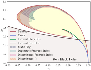
Figure 1. Domain of existence for KBHsSH.
Download figure:
Standard image High-resolution image3.2. Shaded Areas in Detail
3.2.1. Static Ring
On the equatorial plane, if gtt has a local extreme in a region where it is negative (with the metric signature here adopted), then it is clear from Equation (20) that Ω− = 0 at these points. We remark that if gtt > 0, this is an ergoregion, and static orbits are then only possible for spacelike particles. Indeed, the lower boundary of this region in Figure 1 is characterized by the appearance of this second ergoregion with toroidal topology (in addition to the S2 one in the vicinity of the horizon), where the solutions feature an ergo-Saturn as discussed in Herdeiro & Radu (2014a). The transition solutions, i.e., those for which the local maximum of gtt occurs for gtt = 0, contain a ring where massless particles of zero energy can be found inertially at rest, the so-called light points (Grandclément 2017). In Figure 2, we depict the profiles of gtt and gt φ for a solution with such a feature. In these spacetimes, there is both a local minimum and maximum for gtt , and it is possible for a test particle to remain at rest in these regions with respect to a static observer at infinity.
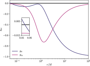
Figure 2. Metric components gtt and gt φ as functions of the normalized radial coordinate r/M for a solution in the gray hatched region for which rH = 0.05. The inset provides a closer look near the horizon marking the existence of an ergoregion, present in every solution for which q < 1.
Download figure:
Standard image High-resolution image3.2.2. Degenerate Prograde Stable Orbits
As discussed above, there are certain KBHsSH for which on the equatorial plane there exists a region with no retrograde orbits, i.e., Ω− > 0. According to Equation (20), if the slope of gtt is positive, then the quantity in the square root will always be less than ∂r gtt , because the slope of gφ φ (which is monotonic) is always positive. Observing gtt in Figure 2, its slope is positive between the two local extrema where the static rings live. Furthermore, it is possible that in some interval of the radial coordinate, both prograde orbits are stable. Therefore, there are degenerate prograde stable orbits, a feature worth discriminating in the parameter space of Figure 1. To better illustrate this behavior, we provide an example in Figure 3 where both Ω± are plotted (only the positive values) and the stable regions are displayed. In this particular case, most of the radial interval with no retrograde orbits is characterized by stable orbits for both Ω±.
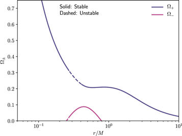
Figure 3. Degenerate prograde stable orbits (Ω− > 0) and stability discontinuity illustrated.
Download figure:
Standard image High-resolution image3.2.3. Discontinuous Prograde Stable Orbits
This region contains solutions for which prograde orbits given by Ω+ suffer from stability discontinuities and is also featured in the example in Figure 3. Specifically, not all orbits are stable for r > rISCO, but instead, there is a region starting and ending with marginally stable orbits where all orbits are unstable. This property is not exclusive to these spacetimes and has previously been reported for axionic solitons (Delgado et al. 2020a) and more recently for Kerr BHs with axion hair (Delgado et al. 2020b), which are a broader class of BHs that includes the set of KBHsSH in the limit of self-interaction coupling.
3.2.4. Discontinuous Existence of Circular Orbits
The three particular cases investigated above arise from the fact that gtt is not monotonic as it usually happens in the exterior region of BHs, that is, it can interchange between negative and positive slopes. Things can get even more interesting when the slope is sufficiently positive such that the square root of Equation (20) becomes zero. This equality occurs when the dragging of the spacetime hits a local extreme and at this point Ω± = ω and locally gt φ ∝ gφ φ . An inertial observer that rotates along with the dragging of the spacetime must have zero angular momentum (L = 0) and therefore is called a zero angular momentum observer (ZAMO). Usually, ZAMOs have nonzero radial velocity and are therefore not in circular motion. In contrast, as can be seen from Equations (17) and (16), in order for them to be in a circular orbit, their energy must be zero. One should also note that ω is the minimum and maximum value that Ω+ and Ω− can achieve, respectively. After this point, Ω± becomes complex and circular orbits are no longer possible for inertial particles until the slope of gtt becomes small enough for yet another point of circularly orbiting ZAMOs to appear. Again, this phenomenon is due to the off-center energy density distribution of the scalar hair. There is a gravitational potential well for each hole and hair, and angular momentum only contributes to a centrifugal force that prevents the particle from maintaining itself at a fixed radius without accelerating. Figure 4 depicts such interrupted existence of circular orbits. Regions where retrograde circular orbits cease to exist have also been found for axion BSs (Delgado et al. 2020a) and Kerr BHs with axion hair (Delgado et al. 2020b).
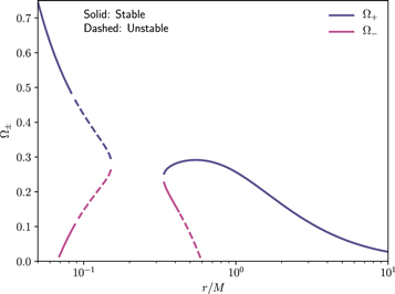
Figure 4. Inertial circular orbits cease to exist whenever  .
.
Download figure:
Standard image High-resolution image4. Results
The thin-disk approach is employed for the solutions lying outside the shaded areas displayed in Figure 1, where the orbital velocity and angular momentum of prograde moving test particles are continuous. Solutions inside the shaded area require a more careful investigation, which might only be possible through dynamical simulations in some cases. For instance, if Ω is discontinuous, the flux is badly defined. Moreover, it would not be reasonable to assume that accreting particles would remain on near-Keplerian orbits in regions of instability or of degenerate prograde stable orbits. One could, however, assume that the ISCO dwells at the radius of the last marginally stable circular orbit, after which all orbits are stable and not degenerate. But such an approach ignores all of the dynamical processes occurring between the horizon and this newly defined ISCO radius, which could host interesting and rich physics whose outcome could possibly be strong enough to shadow the observables extracted from this outer disk. Therefore, a proper investigation of these peculiar solutions will be carried out in future work.
4.1. Radiant Energy Flux
The nonuniqueness of the scalarized solutions for a pair of mass and angular momentum is reflected on the profile of the radiant energy flux for a fixed value of j. In what follows, we present several cases specified by a certain spin parameter and plot it within the flux for BHs of different normalized charges. Although it is not possible to find a general pattern, some particular traits appear in each set. Near the marginally bound clouds, the maximum of the flux decreases with increasing charge, while the opposite is seen in regions far from the clouds in the M versus ωs diagram. The solutions span a large interval of j, but a more prominent set of qualitatively different solutions is concentrated at values slightly lower than the Kerr bound j = 1. In Figure 5, we offer a general view of the maximum value of the normalized flux in the same mass versus ωs diagram we displayed before. Some curves of fixed j are shown for illustration purposes, and we note that for any value j ≤ 1, there will be a small sample of solutions starting at the clouds that are not depicted because they require much higher resolution. Clearly, their sequences are not connected to their respective (same j) sets displayed in different regions above the extremal Kerr line. The exception happens for the particular case of j = 1 that forms two curves connected at the intersection of three points, namely where the lines of extremal Kerr, extremal KBHsSH, and clouds meet. Another interesting case shown here is that of j = 0.8, where far from the clouds the solutions lie somewhat diffusely on a certain region rather than forming a curve. Thus, for a chosen value of the spin parameter, there might be solutions severely different from one another, which can result in radiant energy fluxes of different orders of magnitude. On the lower-left corner of the diagram, the normalized flux for Kerr BHs is shown, and as it is known, it increases monotonically with the spin parameter, e.g., see Equation (27). From the figure, we observe that the maximum normalized flux for KBHsSH can be an order of magnitude higher than that of extremal Kerr BHs.
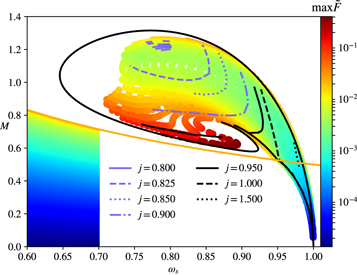
Figure 5. Color plot for the maximum of the normalized flux in the mass vs. ωs diagram. Some solutions of the specific spin parameter are highlighted. On the bottom-left corner, a sample for Kerr black holes is displayed.
Download figure:
Standard image High-resolution imageThe set of solutions starting at the clouds display a profile with decreasing maximum of the flux for increasing charge, and in this case, the bald Kerr BHs feature the strongest radiant energy flux. Sets of lower values of the spin parameter exist only in this region, and an example with j = 0.75 is given in Figure 6, where, as the charge grows larger, the profile flattens out.
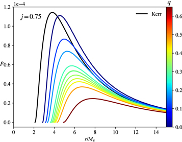
Figure 6. Radiant energy fluxes for j = 0.75 solutions. The color scheme indicates the value of q and therefore how hairy a solution is.
Download figure:
Standard image High-resolution imageThis behavior changes in other regions of the parameter space, as can be seen from Figure 7 where six different examples are given. The top-left panel displays the flux for solutions featuring j = 0.8, which are far from the clouds. As mentioned above, this is a special case where the set does not form a curve crossing a large area of the parameter space in Figure 5 but is concentrated in a more limited region where the solutions are quite similar. Hence, a single behavior is observed in the flux profile as the normalized charge varies, i.e., the larger it is, the higher the peak of the flux gets. The top-right and middle-left panels show solutions for which j = 0.90 and 0.95, respectively. Here we enter the regime where a wider region of the parameter space is crossed by a curve of fixed j. As we notice from the pictures, there is not a unique way of how the flux profile scales with the scalar charge. In the panel for j = 0.90, we display an inset to show the flux corresponding to Kerr, along with those solutions close to the cloud for which the maximum of the flux decreases with increasing charge. More importantly, we notice that the highest flux peak found is over two orders of magnitude greater than the Kerr peak. The middle right panel depicts solutions for which j = 1, a quite special case because here the curve lying near the clouds is connected to the one existing above the extremal Kerr line. Furthermore, we observe that the fluxes are of the same order of magnitude. The bifurcation from the extremal Kerr is made clear: for the solutions lying above this line, the peak of the flux increases with the scalar charge, whereas for those below it, the peak decreases with increasing charge. Nevertheless, we remark that, interestingly, the radius of the ISCO increases in both cases. Finally, in the bottom panel, we show fluxes for solutions with a spin parameter above the Kerr bound, which never approach the clouds but remain mainly in a narrow region of the parameter space for high values of ωs . In these cases, the peak increases with the charge, and we note that, albeit hard to establish numerically, the higher j > 1 is, the larger is the lowest charge found in the solution set.
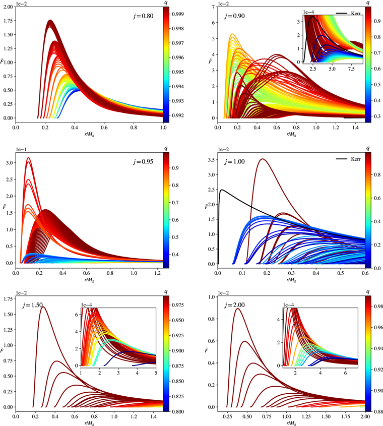
Figure 7. Radiant energy fluxes for solutions of fixed j.
Download figure:
Standard image High-resolution image4.2. Efficiency
BHs offer the most efficient mechanism for converting rest energy into radiation. As stated earlier, this parameter is given by the difference between the particle’s normalized energy at infinity—which is one—and the energy at the ISCO, see i.e., Equation (24). Figure 8 offers the efficiency of KBHsSH against j, where the limiting cases of Kerr BHs and solitons are highlighted in two different curves. Heeding the peculiarities discussed in Section 3, we consider only regular solutions, those lying outside the shaded region of Figure 1. This parameter space is not unique and several solutions can be found for a given pair of (j, ).
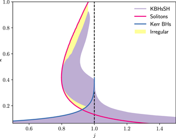
Figure 8. Efficiency vs. j. Note that there is no uniqueness in this domain, i.e., for a pair (j, ).
Download figure:
Standard image High-resolution imageGiven a specific value of j < 1, KBHsSH can always be found below the Kerr curve. At the Kerr bound (and above), all solutions are less efficient than the bald Kerr, in agreement with Figure 7, as the radius of the ISCO increases with the scalar charge. However, for the interval j ∈ (0.8, 1.0), we find a range in the diagram well above the Kerr line, and the highest efficiency found exceeds 90%. This is only possible for BHs with a very small horizon radius and very large scalar charge as they behave more strongly as solitons than BHs, and the ISCO is found at very small radii.
4.3. Luminosity
Let us now evaluate the observed luminosity for a few scalarized BHs. We assume the central object to be a supermassive BH of M = 2.5 × 10⁶
M⊙ and  yr−1, with the plane of the disk oriented at zero degrees with the Euclidean line path to the observer. These values are chosen for illustration purposes only, but we stress that they are fairly conservative (much below the Eddington limit) and reasonable for representing supermassive BHs. We also consider four different cases of fixed spin parameters separately, i.e., j ∈ {0.75, 0.9, 1.0, 2.0}. The results are displayed in Figure 9, together with the curves corresponding to the respective Kerr BH (when applied). For the chosen mass scale and accretion rate, the luminosity peaks at the visible–UV interface part of the electromagnetic spectrum, while stellar-mass BHs with similar mass-accretion rate ratio
  would lie on the X-ray band. In all cases below the Kerr bound, some solutions naturally show negligible differences with the bald BH case (also part of the solution set). As we get farther away from the clouds in the parameter space, though, observable discrepancies arise.
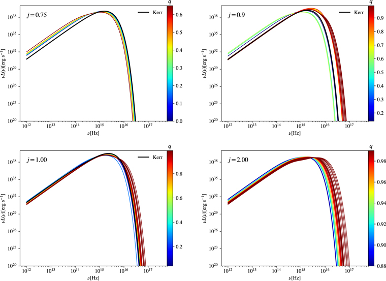
Figure 9. Luminosities for solutions of fixed j.
Download figure:
Standard image High-resolution imageThe particular case of j = 0.75 has a peak in luminosity for q = 0.0 (Kerr BHs). Recall that the efficiency for this spin parameter decreases with the charge, and so does the radiant energy flux. The luminosity curves intersect each other, increasing and decreasing faster for larger charges as the frequency increases. Therefore, at lower frequencies, ν L is higher for larger charges and at higher frequencies, ν L is higher for lower charges. The largest difference in the peak of luminosity between the curves is 36.7% whereas for the peaking frequency, it is 31.6%.
As previously shown, there are many qualitatively different solutions with fixed spin parameters in the interval j ∈ (0.8, 1.0). This is apparent in the luminosity profile as curves can fall either below or above the Kerr case. For j = 0.9 in the examples depicted in the figure, the peak of the luminosity is highest for q = 0.91 and lowest for q = 0.55, with a relative difference of 77.2%, and of 53.3% in the peaking frequency. Extremal Kerr displays the highest luminosity peak among the curves of j = 1.0, but interestingly not the highest-peaking frequency, which is offset by 14.4%. The largest relative difference in the peak of luminosity is of 49.4%. Above the Kerr bound, most solutions are highly scalarized and much closer to a solitonic star than to a bald BH. For j = 2.0, the peak of the luminosity is proportional to the charge, while the peaking frequency decreases with it. In all cases, the differences are much higher at the end of the observed spectrum, and the interval for the cutoff frequencies (where ν L = 0) grows consistently with j, with an interval of 1.25 × 10¹⁶ Hz for j = 0.75 and of 1.5 × 10¹⁷ Hz for j = 2.0.
5. Conclusions
In the present article, we analyzed some features of circular orbit geodesics around KBHsSH and calculated the radiant energy flux and luminosity for several solutions through the thin accretion disk approach. We showed that due to the nonmonotonic behavior of the metric function on the equatorial plane, some peculiar traits appear for a subset of the solutions and categorized them accordingly. Specifically, some solutions feature a static ring, where one of the eigenvalues for the orbital velocity is null; some contain regions where both eigenvalues are positive and the orbit is stable; some contain disconnected regions of stable orbits for the eigenvalue, which is everywhere positive; and finally, some for which there is a region where no real-valued eigenvalues exist and hence no inertial circular orbits are possible. It is unclear how accretion would take place in those backgrounds, and the thin-disk approach is certainly not suitable for most of them, where discontinuities appear for both the orbital velocity and the angular momentum.
The regular solutions, i.e., the set that does not suffer from such discontinuities, were normalized with respect to their masses and analyzed in bundles of the same spin parameter, but with different charges. Wherever j ≤ 1.0, we also computed the quantities that matter for the corresponding Kerr BH. Concerning the flux and luminosity, because of the nonuniqueness of the solutions for any chosen j, many different profiles appear, and although we observe some pattern in their dependence on the scalar charge for smaller or higher j, in the interval j ∈ (0.8, 1.0), large differences appear even for solutions of similar q. The ratio between the largest and smallest peak of the normalized flux is about  .
.
The efficiency of KBHsSH is much varied and always below that of Kerr with the same spin parameter for j < 0.8, and below that of extremal Kerr for j > 1.0. In the interval in between, however, it takes various values, reaching over 90% for some of the hairiest solutions where the ISCO radius approaches that of the horizon, which is already quite small.
The luminosity profiles do not differ strongly enough to peak at different bands of the spectrum or to be over many orders of magnitude apart, but the differences are still significant to be measured. While many results depart very slightly from what is obtained from a Kerr BH (which is part of the solution set), others can peak at lower or higher frequencies, as well as be more or less luminous for some fixed νe and j.
Even though Kerr models fit the data well, the existence of an extra parameter q describing KBHsSH offers a manifold extension in the solution set, which makes it hard to verify, constrain, or dismiss their existence solely based on this kind of observation. On the other hand, once the mass, accretion rate, and angular momentum are well constrained, it is possible to infer from accretion disk observations what the scalar charge of the BH is. Such indirect measurement is fundamental in order to specify a particular compact object because Q cannot be extracted asymptotically from the metric as there is no Gauss law associated with it. By combining the luminosity with other observations such as from the iron Kα line and shadows, one could strongly narrow down the possible solutions with a good enough fit, and assess how KBHsSH performs in contrast to bald Kerr. More stringent constraints are definitely to be expected from future measurements of the geodesic motion of nearby stars. As we have shown with the peculiar structure of circular orbits on the equatorial plane for a subset of solutions, the growth of a massive hair with off-center energy distribution can cause the metric functions to behave nonmonotonically, as opposed to what happens for GR BHs outside the event horizon.
L.C. and D.D. acknowledge financial support via an Emmy Noether Research Group funded by the German Research Foundation (DFG) under grant No. DO 1771/1-1. S.Y. would like to thank the University of Tuebingen for the financial support. S.Y. acknowledges financial support by the Bulgarian NSF Grant KP-06-H28/7. Networking support by the COST Actions CA16104 and CA16214 is also gratefully acknowledged.
Appendix: Radiant Energy Flux in Adapted Spherical Coordinates
The equations describing thin accretion disks widely used in the literature were first derived in Novikov & Thorne (1973), Page & Thorne (1974), where the authors employed adapted cylindrical coordinates near the equatorial plane. Some of these equations are revisited here for a metric written over adapted spherical coordinates because there are a few subtleties one needs to heed. The end result, though, is exactly the same in this approximation regime.
As in the original paper, quantities written inside brackets are averaged over time and the axial coordinate:

The four-velocity of the fluid in its local rest frame,  , is averaged also over the height of the disk and weighted by its rest mass density ρ0,

where Σ is the averaged surface energy density at a certain point:

The energy-momentum tensor of the fluid is written in terms of the averaged four-velocity in general form as

where tμ ν is the averaged energy-momentum tensor in the rest frame and is orthogonal to uμ , and qμ is an energy flux vector field, also orthogonal to the four-velocity.
Among all of the assumptions made and used to derive the equations is the assertion that the disk is optically thick, i.e., the radiation emitted along the disk’s plane is negligible, and one considers only the flux orthogonal to its face (hence, qμ uμ = 0). Thus, the averaged flux of radiant energy is given by
which is simply the tensor transformation from the original vertical flux qz when z ≪ r or θ0 ≈ π/2. Finally, the explicit form of the flux is derived from the conservation laws, yielding