Abstract
We present geometric and dynamical modeling of the broad line region (BLR) for the multi-wavelength reverberation mapping campaign focused on NGC 5548 in 2014. The data set includes photometric and spectroscopic monitoring in the optical and ultraviolet, covering the Hβ, C iv, and Lyα broad emission lines. We find an extended disk-like Hβ BLR with a mixture of near-circular and outflowing gas trajectories, while the C iv and Lyα BLRs are much less extended and resemble shell-like structures. There is clear radial structure in the BLR, with C iv and Lyα emission arising at smaller radii than the Hβ emission. Using the three lines, we make three independent black hole mass measurements, all of which are consistent. Combining these results gives a joint inference of  . We examine the effect of using the V band instead of the UV continuum light curve on the results and find a size difference that is consistent with the measured UV–optical time lag, but the other structural and kinematic parameters remain unchanged, suggesting that the V band is a suitable proxy for the ionizing continuum when exploring the BLR structure and kinematics. Finally, we compare the Hβ results to similar models of data obtained in 2008 when the active galactic nucleus was at a lower luminosity state. We find that the size of the emitting region increased during this time period, but the geometry and black hole mass remained unchanged, which confirms that the BLR kinematics suitably gauge the gravitational field of the central black hole.
1. Introduction
Broad emission lines in active galactic nuclei (AGNs) are thought to arise from the photoionization of gas in a region surrounding a central supermassive black hole. The geometry and dynamics of this so-called broad line region (BLR), however, are not well understood. Since a typical BLR is only on the order of light days in radius, this region nearly always cannot be resolved even in the most nearby AGNs, with rare exceptions (e.g., 3C 273, Gravity Collaboration et al. 2018). Emission-line profiles can provide some information about the line-of-sight (LOS) motions of the gas, but more data are required to extract the BLR structure and dynamics.
The technique of reverberation mapping (Blandford & McKee 1982; Peterson 1993, 2014; Ferrarese & Ford 2005) utilizes the time lag between continuum fluctuations and emission line fluctuations to extract a characteristic size of the BLR. Paired with a velocity measured from the emission-line profile, these data provide black hole mass measurements to within a factor, f. This factor, of order unity, accounts for the unknown BLR structure and dynamics. Velocity-resolved reverberation mapping takes this one step further by breaking up the line profile into velocity bins and studying how each part responds to the continuum. This method has found results that are consistent with gas in elliptical orbits for some objects, while others indicate either inflowing or outflowing gas trajectories (e.g., Bentz et al. 2009; Denney et al. 2009; Barth et al. 2011a, 2011b; Du et al. 2016; Pei et al. 2017). With a similar goal, the code MEMEcho (Horne et al. 1991; Horne 1994) has been used to recover the response function, which describes how continuum fluctuations map to emission-line fluctuations in LOS velocity−time-delay space. Comparing these velocity–delay maps to those produced by various BLR models has pointed toward a similar range of BLR geometries and dynamics (e.g., Bentz et al. 2010; Grier et al. 2013b).
In this work, we utilize an approach to directly model reverberation mapping data using simplified models of the BLR, first discussed by Pancoast et al. (2011, 2012) and Brewer et al. (2011). The goal of this approach is not to model the physics of the gas in the BLR, but rather to obtain a description of the geometry and kinematics of the gas emission. The processes at work within the BLR are likely very complex, and an exhaustive BLR model including numerical simulations would be computationally expensive and time consuming. By using a simple, flexibly parameterized model with a small number of parameters, one can quickly produce emission-line time series and use Markov chain Monte Carlo methods to put quantitative constraints on the kinematic and geometrical model parameters. Realistic uncertainties can still be estimated by inflating the error bars on the spectra with a parameter T, accounting for the limitations of a simplified model.
The dynamical modeling codes described by Pancoast et al. (2014a), used in this work, and Li et al. (2013) have so far been applied to 17 AGNs (Pancoast et al. 2014b, 2018; Grier et al. 2017; Li et al. 2018; Williams et al. 2018). Each BLR in this sample is best fit with models resembling thick disks that are inclined slightly to the observer, despite there being no preference for this geometry built into the modeling code, and all MBH measurements are consistent with those of other techniques. The flexibility of the model is apparent in other parameters, such as model kinematics ranging from mostly inflow to mostly outflow. These applications of dynamical modeling have been limited, however, to a single emission line, Hβ λ4861. Studies of the higher-ionization lines have not been possible due to the lack of the high-quality UV data required for such modeling.
The applications of the modeling approach have all used the optical continuum as a proxy for the ionizing continuum, as all ground-based reverberation mapping studies must do. Recent work monitoring continuum emission at a range of wavelengths has shown a measurable lag between the UV fluctuations and the optical continuum fluctuations (Edelson et al. 2015; Fausnaugh et al. 2016), raising the question of whether the optical continuum is a suitable proxy for the ionizing continuum. In the case of black hole mass measurements based on a scale factor f, the lag is, to first order, removed in the calibration of f with the MBH − σ* relation. This is not the case for the dynamical modeling approach, however, and it is unclear how the continuum light curve choice affects the modeling results.
The AGN Space Telescope and Optical Reverberation Mapping (AGN STORM) Project provides a unique data set that can allow us to address some of the modeling assumptions and extend the modeling approach to higher-ionization portions of the BLR. The AGN STORM Project was anchored by nearly daily observations of the Seyfert 1 galaxy NGC 5548 for six months in 2014 with the Hubble Space Telescope (HST) Cosmic Origins Spectrograph (COS) (De Rosa et al. 2015). Concurrent UV and X-ray monitoring was provided by Swift (Edelson et al. 2015). Ground-based photometry (Fausnaugh et al. 2016) and spectroscopy (Pei et al. 2017) were carried out at a large number of observatories and the UV–optical data were used to study the structure of the accretion disk (Starkey et al. 2017). The UV spectra revealed both broad and narrow absorption features of unusual strength compared to historical UV observations of NGC 5548 and this required careful modeling of the emission and absorption features (Kriss et al. 2019) that will be essential for this paper. These models were also used to recover velocity–delay maps (Horne et al. 2020) for the strong emission lines that are the subject of this paper. Much of the analysis of the AGN STORM data has been with the aim of understanding an anomalous period during the middle of the observing campaign when the emission and absorption lines at least partially decoupled from the continuum behavior, the so-called “BLR holiday” (Goad et al. 2016; Mathur et al. 2017; Dehghanian et al. 2019). In this work, we use both the UV and optical continuum light curves to examine the effect of continuum wavelength choice on the modeling results, and we model the BLRs for three emission lines: Hβ, C iv, and Lyα.
In Section 2 we provide a brief overview of the data we use for the modeling, and in Section 3 we summarize the modeling method used. In Section 4 we present the modeling results for the Hβ, C iv, and Lyα BLRs, and in Section 5 we combine the results to make a joint inference on the black hole mass in NGC 5548. In Section 6 we discuss how the continuum light curve choice affects the modeling results, compare the Hβ results to previous modeling, and discuss the similarities and differences of the three line-emitting regions. Finally, we conclude in Section 7.
2. Data
2.1. Continuum Light Curves
We fit models to the data using two separate continuum light curves. We use a UV light curve to fit models for all three of the emission lines, plus a V-band light curve to fit models to the Hβ light curve. Since the UV light curve is a closer proxy to the actual ionizing continuum, we expect this to be the more realistic physical model. However, the UV is inaccessible to ground-based reverberation mapping campaigns targeting Hβ, and an optical continuum is typically used in its place. Using both continuum light curves allows us to study the effect this has on modeling results.
The UV continuum light curve is constructed by joining the HST 1157.5 Å light curve with the Swift UVW2 light curve. Including the Swift data allows us to extend the light curve back in time to explore the possibility of longer emission line lags. Details of the HST and Swift campaigns can be found in the papers by De Rosa et al. (2015, Paper I) and Edelson et al. (2015, Paper II), respectively. To combine the light curves, we scale the Swift UVW2 light curve to match the HST flux where data overlap in time, and shift the scaled Swift light curve by 0.8 days, the time lag between the Swift UVW2 and HST 1157.5 Å light curves as measured by Fausnaugh et al. (2016, Paper III). The final UV light curve is then the portion of the Swift light curve that lies before the start of the HST campaign, plus the full HST light curve.
The V-band light curve data consist of approximately daily observations obtained with several ground-based telescopes between 2013 December and 2014 August. The details of the optical continuum observing campaign are described by Fausnaugh et al. (2016).
2.2. Emission Lines
We model the line-emitting regions producing three lines—Lyα, C iv, and Hβ. The raw data for Lyα and C iv were obtained using HST COS (Green et al. 2012) from 2014 February 1 to July 27. Due to the strong absorption features in the UV lines that can influence our modeling results, we use the broad emission-line models of Lyα and C iv from Kriss et al. (2019, Paper VIII). The emission lines we use in this paper are the sum of several Gaussian components, namely components 30–38 for C iv and components 5–9 for Lyα. The uncertainties are then calculated following the prescription of Kriss et al. (2019).
The ∼15,000 resolving power of HST COS renders modeling the UV lines at full resolution computationally infeasible given our current BLR model. We therefore bin the Lyα and C iv spectra by a factor of 32 in wavelength to reduce this computational load. Since we are only interested in the larger-scale features of the BLR and emission-line profile, no relevant information is lost in this step. For C iv (Lyα), we model the spectra from 1500.8 to 1648.6 Å (1180.7–1278.8 Å) in observed wavelength, giving 95 (80) pixels across the binned spectrum. In LOS velocity, this is −14,000 to 13,900 km s−1 (−13,600 to 10,100 km s−1).
The optical spectroscopic observing campaign is described in detail by Pei et al. (2017, Paper V) and is summarized briefly here. The Hβ spectra were obtained from 2014 January 4 through July 6 with roughly daily cadence using five telescopes. The resulting spectra were decomposed into their individual components to isolate the Hβ emission from other emission features in the spectral region. Pei et al. (2017) fit models using three templates for Fe ii, but found the template from Kovačević et al. (2010) provided the best fits. We therefore use this version of the spectral decomposition for this work. To produce the spectra used in this work, we take the observed spectra and subtract off all modeled components except for the Hβ components. There are strong [O iii] residuals at wavelengths longer than 5010 Å, so we only model the spectra from 4775.0 to 5008.75 Å in observed wavelength, totaling 188 pixels across the emission line. In LOS velocity, this is −10,300 to 3900 km s−1. While this means we do not use the information contained in the spectra redward of 5008.75 Å to constrain the BLR model, the model still produces a full emission-line profile including the red wing.
2.3. Anomalous Emission-line Behavior
As discussed in several of the papers in this series, the broad emission lines appear to stop tracking the continuum light curve part way through the observing campaign (Goad et al. 2016; Mathur et al. 2017; Dehghanian et al. 2019). Our model of the BLR assumes that the BLR particles respond linearly and instantaneously to all changes in the continuum flux. Since the anomalous behavior of NGC 5548 is a direct violation of this assumption, we fit our models using only the portion of the spectroscopic campaign in which the BLR appears to be behaving normally. For this work, we use a cutoff date of THJD = 6743 (THJD = HJD − 2,450,000), as determined for Hβ by Pei et al. (2017). The time of de-correlation was measured to be slightly later at THJD = 6766 for C iv, but for continuity we use the THJD = 6743 cutoff for all three lines. In the case of Hβ, we also attempt to model the full spectral time series, but these models fail to converge.
3. The Geometric and Dynamical Model of the BLR
We fit the same BLR model to all three emission lines, allowing us to directly compare the parameters for each line-emitting region. A full description of the BLR model is given by Pancoast et al. (2014a), and a summary is provided here.
3.1. Geometry
The BLR is modeled as a distribution of massless point-like particles surrounding a central ionizing source at the origin. These are not particles meant to represent real BLR gas, but rather a way to represent emission-line emissivity in the BLR. The point particles are assigned radial positions, drawn from a Gamma distribution
and shifted from the origin by the Schwarzschild radius Rs = 2G MBH/c2 plus a minimum radius rmin. To work in units of the mean radius, μ, we perform a change of variables from (α, θ, rmin) to (μ, β, F)


where β is the shape parameter and F is the minimum radius (rmin, typically a few light days) in units of μ. We assume that the observing campaign is sufficiently long enough to measure time lags throughout the whole BLR, so we truncate the BLR at an outer radius  , where Δtdata is the time between the first continuum light-curve model point and the first observed spectrum. Note that this is not an estimate of the outer edge of BLR emission, and for all cases with campaigns of sufficient duration, the emission trails to near-zero at much smaller radii than rout. The values of rout are reported in Table 1.
Table 1. BLR Model Parameter Values
| Parameter | Brief Description | Lyα | C iv | Hβ versus UV | Hβ versus V-band |
|---|---|---|---|---|---|

|
Black hole mass |

|

|

|

|
 ( ( ) ) |
Mean line emission radius |

|

|

|

|
 ( ( ) ) |
Median line emission radius |

|

|

|

|
 ( ( ) ) |
Minimum line emission radius |

|

|

|

|
 ( ( ) ) |
Radial width of line emission |

|

|

|

|
 ( ( ) ) |
Mean lag in observer frame |

|

|

|

|
 ( ( ) ) |
Median lag in observer frame |

|

|

|

|
| β | Shape parameter of radial distribution (Equation (3)) |

|

|

|

|
 ( ( ) ) |
Half-opening angle |

|

|

|

|
 ( ( ) ) |
Inclination angle |

|

|

|

|
| κ | Cosine illumination function parameter (Equation (6)) |

|

|

|

|
| γ | Disk face concentration parameter (Equation (5)) |

|

|

|

|
| ξ | Mid-plane transparency |

|

|

|

|

|
Elliptical orbit fraction |

|

|

|

|

|
Inflow/outflow flag |

|

|

|

|
 ( ( ) ) |
Angle in  plane plane |

|

|

|

|

|
Turbulence (Equation (7)) |

|

|

|

|
 
|
Outer line emission radius (fixed parameter) | 145 | 145 | 81 | 80 |
| T | Temperature (statistical) | 5000 | 500 | 300 | 200 |
Note. Median and 68% confidence intervals for the main BLR model parameters. Note that rout is a fixed parameter, so we do not include uncertainties, and we also include the temperature T used in post-processing.
Download table as: ASCIITypeset image
Next, the full plane of particles is inclined relative to the observer’s LOS by an angle θi, such that a BLR viewed face-on would have θi = 0 deg. The particles are distributed around this plane with a maximum height parameterized by a half-opening angle θo. The angle above the BLR midplane for an individual particle as seen from the black hole is given by

where U is drawn from a uniform distribution between 0 and 1 and γ is a free parameter between 1 and 5. In the case of γ = 1, the point particles are evenly distributed between the central plane and the faces of the disk at θo, while for γ = 5, the particles are clustered at θo.
The emission from each individual particle is assigned a weight between 0 and 1 according to

where ϕ is the angle measured between the observer’s line to the origin and the particle’s line to the origin, and κ is a free parameter between −0.5 and 0.5. For  , particles preferentially emit back toward the ionizing source, and for
  , particles preferentially emit away from the ionizing source.
Additionally, we allow for the presence of an obscuring medium in the plane of the BLR, such as an optically thick accretion disk, that can block line emission from the far side. The mid-plane can range from transparent to opaque according to the free parameter ξ, ranging from 0 (fully opaque) to 1 (fully transparent). To improve computation time, this is achieved by reflecting a fraction of the particles across the BLR midplane from the far side to the near side.
3.2. Dynamics
The wavelength of emission from each particle is determined by the velocity component along the observer’s LOS. To determine the velocities, we first split the particles into two subsets. A fraction fellip are set to have near-circular elliptical orbits around the black hole, with radial and tangential velocities drawn from Gaussian distributions centered on the circular velocity in the vr − vϕ plane. Since the circular velocity depends on the particle position and the black hole mass, MBH enters as a free parameter in this step.
The remaining 1 − fellip particles are assigned to have either inflowing or outflowing trajectories. In this case, the velocity components are drawn from a Gaussian centered on the radial inflowing or outflowing escape velocity in the vr − vϕ plane (see Pancoast et al. 2014a, Figure 2, for an illustration). Inflow or outflow is determined by the binary parameter fflow, where fflow < 0.5 indicates inflow and fflow > 0.5 indicates outflow. Additionally, we rotate the velocity components by an angle θe in the vr − vϕ plane toward the circular velocity, increasing the fraction of bound orbits as θe increases toward 90°.
We include a contribution from macroturbulent velocities with magnitude

where  is the circular velocity and
  is the normal distribution with mean 0 and standard deviation σturb, a free parameter. This value is calculated for each particle and added to its LOS velocity.
Doublet emission lines are accounted for by producing flux shifted in wavelength relative to both doublet rest wavelengths. Thus, the particles in the C iv λλ 1548,1550 BLR model use both 1548 Å and 1550 Å as the reference wavelength.
3.3. Producing Emission-line Spectra
The ionizing source is assumed to be a point source at the origin that emits isotropically and directly follows the AGN continuum light curves described in Section 2.1. This light propagates out to the BLR particles which instantaneously reprocess the light and convert it into emission-line flux seen by the observer. There is a time lag between the continuum emission and the line emission determined by the particles’ positions, and the wavelength of the light is Doppler shifted from the central emission-line wavelength based on the particle’s LOS velocity. In the case of C iv, both components of the doublet emission line are included.
Since the BLR particles can lie at arbitrary distances from the central ionizing source, we need a way to calculate the continuum flux at arbitrary times. We use Gaussian processes as a means of flexibly interpolating between points in the observed continuum light curve as well as extending the light curve to times before or after the start of the campaign to explore the possibility of longer lags. The Gaussian process model parameters are included in our parameter exploration which allows us to include the continuum interpolation uncertainty in our inference of the other BLR model parameters.
3.4. Exploring the Model Parameter Space
For each set of model parameters, we use 4000 BLR test particles to produce an emission-line time series with times corresponding to the actual epochs of observation. We can compare the observed spectra with the model spectra using a Gaussian likelihood function and adjust the model parameters accordingly. To explore the BLR and continuum model parameter space, we use the diffusive nested sampling code DNest4 (Brewer & Foreman-Mackey 2016). Diffusive nested sampling is a Markov chain Monte Carlo method based on nested sampling that is able to efficiently explore high-dimensional and complex parameter spaces.
DNest4 allows us to do further analysis in post-processing through the introduction of a temperature T, which softens the likelihood function by dividing the log of the likelihood by T. The temperature in this case is not a physical temperature, but rather a parameter commonly used in optimization algorithms such as simulated annealing (Kirkpatrick et al. 1983). In the case of a Gaussian likelihood function, this is equivalent to multiplying the uncertainties on the observed spectra by  . This factor can account for under-estimated uncertainties on the spectra or the inability of the simplified model to accurately fit the complexities of the real data.
The value of T is determined by examining the sample distributions at increasing levels of likelihood and choosing the largest T for which the distributions remain smooth and do not contain several local minima. The choices of T for each run are listed in Table 1. In the cases of Lyα and C iv, we required very large temperatures due to the inability of the simple model to fit the level of detail present in the high signal-to-noise ratio HST data.
Convergence of the modeling runs was determined by ensuring that the parameter distributions for the second half of each run matched the parameter distribution for the first half of the run.
4. Results
In this section, we describe the results of fitting our BLR model to the data. For each emission line, we give the posterior probability density functions (PDFs) for the model parameters and use these to draw inferences on the structural and kinematic properties of the BLRs. From the posterior samples, we show one possible geometric structure of the BLR gas emission, selected to have parameter values closest to the median inferred values. We also show the transfer function, Ψ(λ, τ), which describes how continuum (C) fluctuations are mapped to emission-line (L) fluctuations as a function of wavelength and time delay:

The functions shown are calculated by producing transfer functions for 30 random models from the posterior and calculating the median value in each wavelength–delay bin. Table 1 lists the inferred model parameters for each line-emitting region.
4.1. Hβ
Multi-wavelength monitoring campaigns have shown that longer continuum wavelengths tend to lag behind shorter wavelengths (e.g., Edelson et al. 2015, 2017; Fausnaugh et al. 2016, 2018), indicating that the UV is a closer proxy to the ionizing continuum than the V band. Additionally, the shorter-wavelength continuum variations show more short-timescale structure than longer wavelengths. Since the emission lines respond to the short-timescale ionizing continuum variations, one could observe higher-frequency emission-line variability than is present in the smoothed V-band continuum light curve. Complicating matters even further, recent studies have shown that diffuse continuum emission arising in the BLR gas can be strong enough to significantly enhance continuum lags, especially at optical wavelengths (Korista & Goad 2001, 2019; Cackett et al. 2018; Lawther et al. 2018).
When the V band is used, these combined effects can lead to shorter Hβ–optical lags and may result in MBH underestimates if not accounted for. However, since the UV is not available for ground-based reverberation mapping campaigns, the V band is very often used as a proxy for the ionizing continuum. Since both light curves are available in the AGN STORM data set, we have a unique opportunity to compare the modeling results using each continuum light curve. We run our modeling code with the Hβ emission-line data using both the UV and V-band light curves as the driving continuum to study potential systematics introduced by the choice of continuum wavelength.
4.1.1. Hβ versus UV Light Curve
For the first Hβ modeling tests, we use the HST 1157.5 Å plus Swift UVW2 light curve as the driving continuum. The data require a temperature of T = 300, equivalent to increasing the spectral uncertainties by a factor of  . As shown in Figure 1, our model fits the rough shape of the emission-line light curve, but there is clear structure in the residuals near the line peak. Additionally, there is a small trough in the emission-line data at wavelengths just short of the line peak that the models are unable to reproduce. Looking at the integrated Hβ flux light curve, we see that the models can reproduce the general structure of the variations, but the full amplitude of variations is not perfectly matched. In particular, the fluctuations in the first half of the Hβ light curve are larger than those predicted by the models, while the same models are able to reproduce the larger-scale rise and fall in the second half of the light curve.
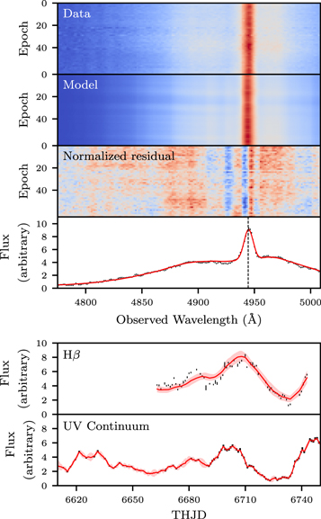
Figure 1. Numbered 1–6 from top to bottom, panels 1–3: observed Hβ emission-line profile by observation epoch, the profiles produced by one possible broad line region model, and the normalized residual (![$[\mathrm{Data}-\mathrm{Model}]/\mathrm{Data}\,\mathrm{uncertainty}$](https://content.cld.iop.org/journals/0004-637X/902/1/74/revision1/apjabbad7ieqn102.gif) ). Panel 4: observed Hβ profile of the 10th epoch (black) and the emission-line profile produced by the model shown in panel 2 (red). The vertical dashed line shows the emission line center in the observed frame. Panel 5: time series (
). Panel 4: observed Hβ profile of the 10th epoch (black) and the emission-line profile produced by the model shown in panel 2 (red). The vertical dashed line shows the emission line center in the observed frame. Panel 5: time series ( ) of the integrated Hβ emission line data (black) and the integrated Hβ model shown in panel 2 (red). Panel 6: same as panel 5, but with the continuum flux rather than integrated Hβ flux. In panels 4–6, the light red band shows the 1σ scatter of all models in the posterior sample.
Download figure:
Standard image High-resolution imageGeometrically, we find a BLR with a thick disk structure that is highly inclined relative to the observer (Figure 2). The opening angle posterior PDF has a primary peak at 35° and a small secondary peak near 90° (Figure 3, blue lines). Similarly, the inclination angle posterior PDF has a primary peak at 45° and a small secondary rise toward 80°. Simply taking the median and 68% confidence intervals for these parameters gives  deg and
  deg.
deg.
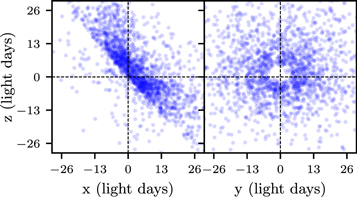
Figure 2. Possible geometry for the Hβ-emitting broad line region (BLR), when modeled using the UV light curve. The left-hand panel shows an edge-on view with the observer on the positive x-axis, and the right-hand panel shows a face-on view of the BLR, as seen by the observer. The size of the circles represents the relative amount of emission from the particles, as seen by the observer. This value is determined by the particle’s position and the parameter κ (Equation (6)). Note that few particles are shown in the bottom-left portion of the left-hand panel due to how the code handles an opaque mid-plane.
Download figure:
Standard image High-resolution image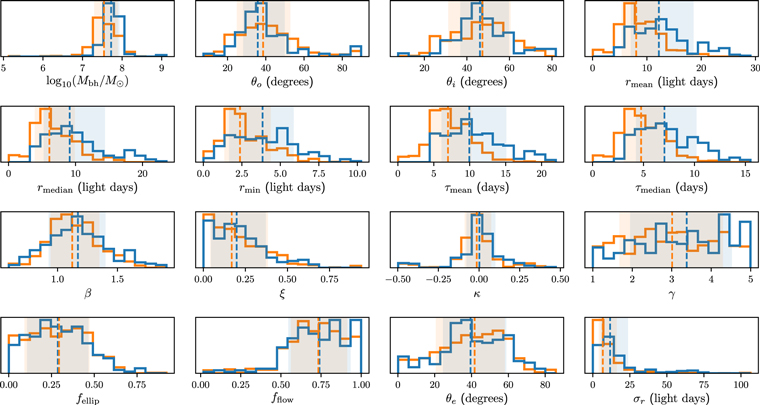
Figure 3. Comparison of the posterior probability density functions for the BLR model parameters obtained when using the UV (blue) and V band (orange) as the continuum light curve driving the Hβ variations. The vertical dashed lines show the median parameter values, and the shaded regions show the 68% confidence intervals.
Download figure:
Standard image High-resolution imageThe median radius of the BLR is  lt-days with an inner minimum radius of
  lt-days. The radial width of the BLR is
  lt-days, and the radial distribution of BLR particles is close to exponential with
  . The relative distribution of particles within the disk (either uniformly distributed or concentrated near the opening angle) is not constrained (
 ). We find a preference for isotropic emission from all BLR particles, rather than emission back toward or away from the ionizing source (
 ). In previous modeling of the Hβ BLR in other AGNs (Pancoast et al. 2014b, 2018; Grier et al. 2017; Williams et al. 2018), nearly every object in which κ is well determined has
  at the 1σ level or greater. This is also the result that is predicted from photoionization models, so we discuss the value from this work further at the end of the section. Finally, models with an opaque midplane are preferred over those without, with
  .
.
Kinematically, the data prefer models in which a third of the BLR particles are on elliptical orbits ( ). The remaining particles are mostly outflowing, with
  , although some of these may still be on bound, highly elliptical orbits, with
  deg. We find little contribution from macroturbulent velocities, with
  ). Finally, we measure the black hole mass in this model to be
  .
.
The Hβ versus UV lag one would measure from the models is  days. This agrees with the Pei et al. (2017) measurements of
  days from cross-correlation and
  days from JAVELIN (Zu et al. 2011). Both of these measurements used the
  light curve as the driving continuum and the Hβ spectra up to THJD = 6743, the same dates used to fit our models. To measure a black hole mass, (Pei et al. 2017) use the cross-correlation lag between Hβ and the 5100 Å continuum, and calculate
  (
(![${\mathrm{log}}_{10}[{M}_{\mathrm{BH}}/{M}_{\odot }]={7.88}_{-0.13}^{+0.10}$](https://content.cld.iop.org/journals/0004-637X/902/1/74/revision1/apjabbad7ieqn124.gif) ), which is consistent with our measurement.
), which is consistent with our measurement.
Horne et al. (2020) find velocity–delay maps that they interpret as indicating a BLR with inclination angle i = 45 degrees, a 20 lt-day outer radius with most response between 5 and 15 days, and black hole mass 
 ]. Our black hole mass and inclination angle measurements agree with these values, but we do find models with BLR emission extending to radii greater than 20 lt-days. We remind the reader that rout in our model is a fixed parameter determined by the campaign duration and should not be interpreted as a measurement of the BLR outer radius.
The transfer function produced by our model (Figure 4(a)) shows that the emission is enclosed within a virial envelope, similar to the maps of Horne et al. (2020). There is a slight angle to the transfer function, showing more emission at short lags and bluer wavelengths, which can be interpreted as an outflow. This agrees with the  and fflow values in the model. Compared with the velocity-resolved measurements of Pei et al. (2017, Figure 10), our plot of the mean delay is noticeably lacking the distinct “M” shape with short lags at the core of the emission line. One way to achieve such a shape is if the far side of the BLR does not respond to the continuum, possibly due to an obscurer. Our simple model is unable to produce such an asymmetric effect, so it is possible that the κ parameter was pushed to greater values in order to dampen the response of the far side.
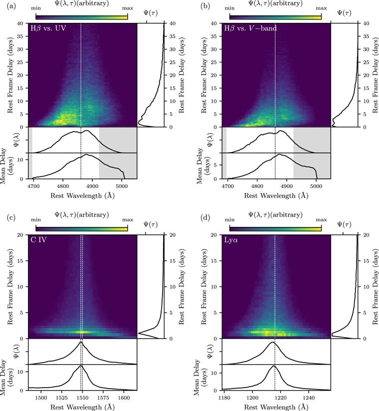
Figure 4. Median transfer functions for each BLR, calculated by producing transfer functions for 30 random models from the posterior and calculating the median value in each wavelength–delay bin. The bottom panels show the lag-integrated transfer function, Ψ(λ), and the mean rest frame lag as a function of wavelength. The right-hand panel shows the velocity-integrated response, Ψ(τ), as a function of rest frame lag. The grayed-out regions indicate the wavelength range that was not modeled for Hβ, and vertical dashed lines show the emission line center.
Download figure:
Standard image High-resolution image4.1.2. Hβ versus V-band Light Curve
For the second Hβ modeling tests, we use the V-band light curve as the driving continuum, with the same Hβ spectra up until the Pei et al. (2017) cutoff. We use a temperature T = 200, corresponding to an increase in spectral uncertainties of a factor  . Similar to the Hβ versus UV models, the Hβ versus V-band models are able to reproduce the large-scale shape of the emission-line profile, but they are unable to fit the smaller-scale wiggles (Figure 5). Again, the amplitude of fluctuations in the Hβ light curve is not fully reproduced in the V-band-driven models, although the general structure is still well captured. In general, the V-band-driven models produce integrated emission-line light curves that are smoothed compared to the UV-driven counterparts.
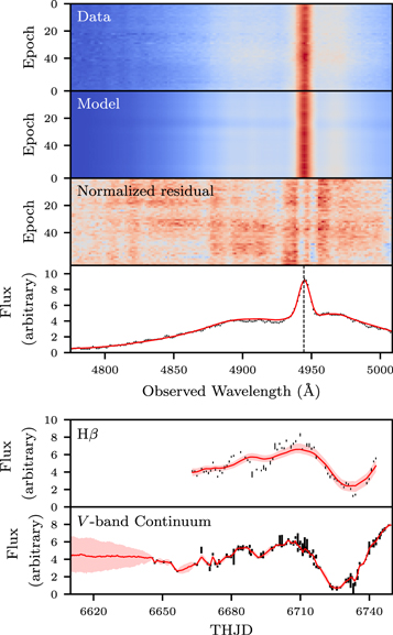
Figure 5. Same as Figure 1, but for the Hβ models using the V band as the driving continuum. The large scatter in modeled continuum light curves before THJD ∼ 6650 is due to extrapolation to times before the monitoring campaign started.
Download figure:
Standard image High-resolution imageGeometrically, models with an inclined thick disk structure are preferred, with  deg and
  deg (Figure 6). The median radius is
  lt-days, the minimum radius is
  lt-days, and the radial width is
  lt-days. The radial distribution is close to exponential with
  and the distribution of particles within the disk is not constrained (
 ). The BLR particles emit isotropically (
 ), and there is a preference for an opaque midplane (
 ).
).
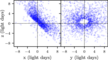
Figure 6. Same as Figure 2, but for the Hβ-emitting BLR modeled using the V-band light curve as the driving continuum.
Download figure:
Standard image High-resolution imageDynamically, models with roughly a third of the particles on elliptical motions are preferred ( ), and the remaining particles are outflowing
  , although many may be on highly elliptical bound orbits (
 degrees). There is little contribution from macroturbulent velocities, with
  . The black hole mass in this model is
  . The transfer function for this model is very similar to those of the models that use the UV light curve as the driving continuum, but the preference for outflow is slightly more pronounced.
The emission line lag one would measure from the models is  days. Within the uncertainties, this agrees with the cross-correlation and JAVELIN measurements of
  and
and  days from Pei et al. (2017). Our black hole mass is formally consistent with their measurement of
  , but slightly smaller for the reason described below.
If  and
and  are the masses measured using the UV and V-band continua, respectively, we expect to find
  . Since the lag between the UV and V-band continua is
  , we can write
Using  days from Fausnaugh et al. (2016) and
  , we expect a difference in
  measurements
  solely due to the UV–optical continuum lag. Our measurements are consistent with this difference.
4.2. C iv (versus UV Light Curve)
The C iv emission line has many absorption features that can affect the modeling results. We therefore use the models from Kriss et al. (2019), using the components corresponding to the C iv emission line. Due to the high spectral resolution of the data, we also bin the emission-line spectra by a factor of 32 in wavelength. This decreases the run-time of the modeling code not only by reducing the number of data points, but also by reducing the number of BLR test particles that would be required to fit such high-resolution data. We use a temperature of T = 500, which is equivalent to increasing the uncertainties by a factor of  .
.
Figure 7 shows the model fits to the C iv emission-line data. Note that while the emission line appears to be single-peaked in the figure due to the binning, both peaks are accounted for in the modeling code. Since the UV emission-line light curves are shorter than the ground-based optical emission-line light curves, there are fewer features allowing the code to determine the time lag and hence the radius of the BLR. The one strong up-and-down fluctuation in the C iv light curve is well captured by our model.
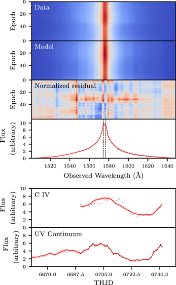
Figure 7. Same as Figure 1, but for the C iv BLR models.
Download figure:
Standard image High-resolution imageGeometrically, the C iv BLR has a thick disk structure ( degrees, Figure 8) that is inclined relative to the observer’s LOS (
 deg), similar to the results for Hβ (Figure 9). The radial distribution, however, has a shape parameter of
  , indicating a very steep drop-off in the density of BLR emission close to rmin. The median radius of the BLR is
  lt-days with an inner minimum radius of
  lt-days. Formally, the standard deviation of the radial distribution of particles is
  lt-days, although this is likely biased high due to the long tails of the distribution. There is a slight preference for the particles to be concentrated near the opening angle, but this parameter is not well determined (
 ). There is a strong preference for emission back toward the ionizing source with
  , and there is no preference for an opaque or transparent midplane (
 ).
).
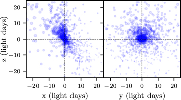
Figure 8. Same as Figure 2, but for the C iv-emitting BLR.
Download figure:
Standard image High-resolution image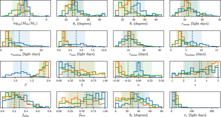
Figure 9. Comparison of the posterior probability density functions for the parameters of the Hβ (blue), C iv (orange), and Lyα (green) BLR models, all using the UV light curve as the driving continuum. The vertical dashed lines show the median parameter values, and the shaded regions show the 68% confidence intervals.
Download figure:
Standard image High-resolution imageThe data prefer models in which roughly a quarter of the BLR particles are on elliptical orbits ( ). Perhaps surprisingly, C iv shows the weakest evidence for outflow, with
  . This can be seen in the transfer functions in which there is a weak preference for inflow, with shorter responses at longer wavelengths. There is little contribution from macroturbulent velocities, with
  ). From this model, we obtain a black hole mass of
  .
.
The C iv emission-line lag is  days. This is consistent with the Kriss et al. (2019) cross-correlation measurement of
  days, measured using the same C iv emission-line models. We should note that they use a slightly longer campaign window ending at THJD = 6765 rather than 6743, but this is unlikely to introduce a large change in the lag measurement.
Compared to the results of Horne et al. (2020), we find a smaller C iv BLR inclination angle ( deg versus i = 45 deg), but we note that Horne et al. (2020) do not estimate uncertainties in their inclination angle fits. We also find a stronger C iv response at shorter delays (<5 days) in our models. This is evident in the velocity-integrated transfer function (Figure 4(c), right panel) with the sharp peak in response at 1–2 days.
4.3. Lyα (versus UV Light Curve)
As with C iv, we use the models from Kriss et al. (2019) for our Lyα data, binned by a factor of 32. The model is able to fit the overall shape of the emission line quite well. The overall shape of the emission line light curve is captured, but many of the models are unable to reproduce the amplitude of the emission line fluctuations (Figure 10, panel 5). In order to fit the data without falling into local maxima in the likelihood space, we soften the likelihood with a temperature of T = 5000, which is equivalent to increasing the uncertainties on the spectra by a factor of  . Including such a high temperature allows us to measure realistic uncertainties on the model parameters.
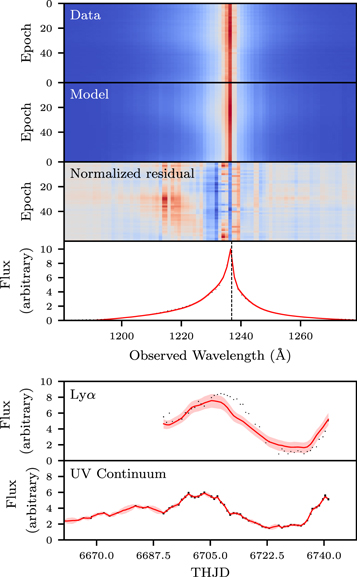
Figure 10. Same as Figure 1, but for the Lyα BLR models. The residuals at 1216 Å are likely due to geocoronal Lyα emission.
Download figure:
Standard image High-resolution imageWe find a Lyα BLR structure that is an inclined thick disk, with  deg and
  deg (Figure 11). The radial distribution of particles drops off very quickly with radius, with
  . The median radius of the BLR particles is
  lt-days, the minimum radius is
  lt-days, and the radial width is
  lt-days. There is a small preference for emission back toward the ionizing source, with
  . There is little preference for the particles to be either uniformly distributed within the thick disk or located near the opening angles (
 ), nor is there a significant preference for either a transparent or opaque midplane (
 ).
).
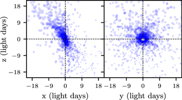
Figure 11. Same as Figure 2, but for the Lyα-emitting BLR.
Download figure:
Standard image High-resolution imageDynamically, most of the particles are on either inflowing or outflowing trajectories ( ), but it is not determined which direction of flow dominates (
 ). As with the models of the BLRs of the other lines, there is little contribution from macroturbulent velocities, with
  . The black hole mass based on the Lyα BLR models is
The models produce an emission-line lag of  days, which is consistent with the Kriss et al. (2019) cross-correlation measurement of
  days. Similar to C iv, we find a smaller Lyα BLR inclination angle than Horne et al. (2020) (
 deg versus i = 45 deg), but the values are still consistent due to the large uncertainty on our measurement and the lack of error bars by Horne et al. We also find a shorter response than Horne et al. for Lyα, with our model response peaking within 5 days, but the significance is difficult to asses without uncertainty estimates.
5. Joint Inferences on the BLR Model Parameters
Ideally, our BLR model would reproduce all three emission lines and we would calculate the likelihood over all three data sets and adjust the model parameters for each region simultaneously. Since we do not know which model parameters should be tied together, modeling each region individually provides a check on the consistency of the modeling method. While the driving continuum used for each BLR model is the same, the spectra are all independent, and we can use the results from the three emission lines to put joint constraints on the model parameters.
5.1. Black Hole Mass
Of all the BLR model parameters, we know that the black hole mass should be the same for all three emission lines. Assuming that the three emission-line time series are independent, we can write

where  ,
,  ,
,  are the data for Hβ, C iv, and Lyα, respectively. We use the Hβ BLR models fit with the UV continuum light curve so that the continuum data are the same for each emission line. The BLR model uses a uniform prior in the log of
  , so
, so
In practice, we estimate the posterior PDFs for the three emission lines using a Gaussian kernel density estimate (KDE) and multiply the three KDEs to obtain a joint constraint on the black hole mass. The resulting joint posterior PDF is shown in Figure 12. The individual  measurements are all consistent with each other, and together provide a joint measurement of
  .
.
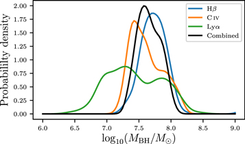
Figure 12. Joint inference on  from combining the posterior probability density functions for the three emission-line region models.
Download figure:
Standard image High-resolution imageUsing our joint constraint on the black hole mass, we can use the method of importance sampling (see, e.g., Lewis & Bridle 2002) to further constrain the other parameters of our BLR models. Importance sampling is a technique that allows one to sample an unavailable distribution P2 via a distribution P1 that can be more easily sampled. By writing  , we simply need to determine the weighting factor
  . In our case, P2 is the posterior PDF for the BLR parameters for, say, Hβ, given all emission-line data:

and P1 is the posterior PDF given only the Hβ data:

Here,  are the Hβ BLR model parameters not including the black hole mass. The weight
  is simply the ratio of our joint PDF on
  to the PDF based on the individual lines.
The result of this method is that the posterior samples with  in regions of high density in the joint PDF will be weighted higher than those with MBH in regions of lower density. This can be useful to exclude regions of parameter space that might fit the emission-line time series well, but with an incorrect black hole mass. Gaussian KDE fits to the original and importance sampled posterior PDFs are shown in Figures 13–15.
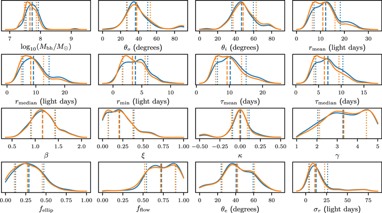
Figure 13. Gaussian kernel density estimate fits to the weighted (orange) and unweighted (blue) posterior probability density functions for the Hβ BLR model parameters with the UV light curve as the driving continuum. The weighting scheme used is the one described in Section 5.1 in which the black hole masses for all three BLR models are forced to be the same. The vertical dashed lines show the median value and the dotted lines show the 68% confidence interval.
Download figure:
Standard image High-resolution image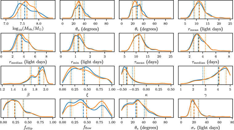
Figure 14. Same as Figure 13, but for the C iv BLR models. The weighting scheme used is the one described in Section 5.1 in which the black hole masses for all three BLR models are forced to be the same.
Download figure:
Standard image High-resolution image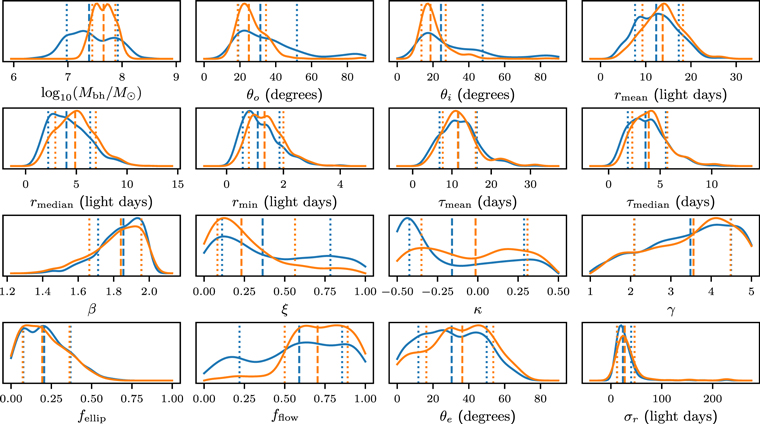
Figure 15. Same as Figure 13, but for the Lyα BLR models. The weighting scheme used is the one described in Section 5.1 in which the black hole masses for all three BLR models are forced to be the same.
Download figure:
Standard image High-resolution imageExamining the weighted results, we find little change to the Hβ BLR parameters, other than a slight decrease in the parameters indicating the size of the BLR. The joint constraint on the black hole mass is slightly lower than the individual Hβ constraint, so this results in preferring BLR geometries that are slightly smaller. The C iv BLR parameters also show almost no change. The posterior PDFs for the Lyα BLR parameters show the largest change due to the largest difference between the Lyα-only MBH PDF and the joint PDF. The solutions with low MBH are essentially excluded, resulting in a very slight increase in radius, and a more robustly determined low inclination angle. Additionally, the kinematics go from being relatively undetermined toward a preference for outflow.
5.2. Black Hole Mass and Inclination Angle
We can also examine the scenario in which both the black hole mass and the inclination angle are assumed to be the same for each line-emitting region. We follow the same methods discussed in Section 5.1, except in this case we examine the 2D posterior PDF for  . Figure 16 shows the Gaussian KDE fits to the 2D posterior PDFs, as well as the joint posterior PDF. From the figure, we see that there is little overlap between the Hβ model parameters and the C iv and Lyα model parameters. Thus, when we calculate the weights to importance sample the Hβ BLR posterior PDFs, only a very small portion of the parameter space receives a significant weight.
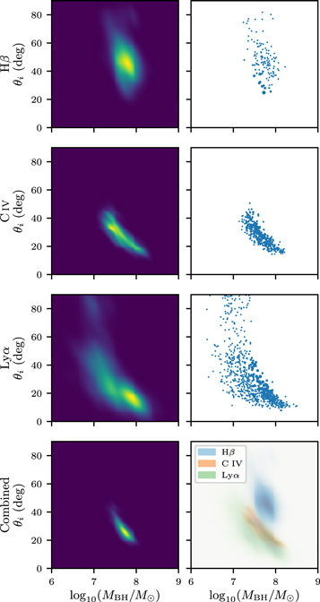
Figure 16. Left: Gaussian kernel density estimates for the 2D posterior probability density functions (PDFs) for  in each BLR model as well as the joint constraint (bottom). Right: weighted posterior samples for the three BLR models (top 3), and the region of overlap of the PDFs in the left column (bottom). The size of each point corresponds to the sample’s weight. The weighting scheme used is the one described in Section 5.2 in which the black hole masses and inclination angles for all three BLR models are forced to be the same.
Download figure:
Standard image High-resolution imageExamining the weighted posterior PDFs in Figure 17, we see that only models with extremely small Hβ BLRs are not excluded. In fact, for the Hβ BLR inclination angle to match that of C iv and Lyα, the Hβ-emitting BLR would need to be smaller than the C iv- and Lyα-emitting BLRs. This directly contradicts the plentiful studies showing ionization stratification within the BLR (e.g., Clavel et al. 1991; Reichert et al. 1994). Additionally, this would require an Hβ lag of  days, which is significantly shorter than the measurements of
  days and
  days by Pei et al. (2017). Given these contradictions as well as the clear offset in the
  posterior PDFs, we conclude that the assumption of identical
  must be faulty.
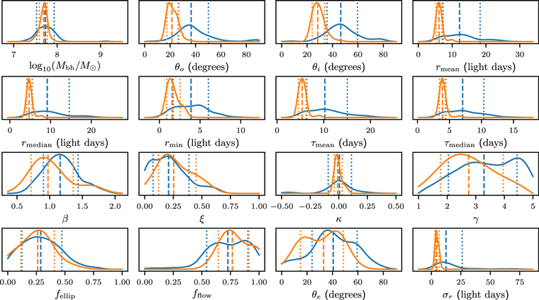
Figure 17. Same as Figure 13, for the Hβ BLR models, but when both MBH and θi are forced to be the same as those inferred by the Lyα and C iv models (described in Section 5.2).
Download figure:
Standard image High-resolution image6. Discussion
6.1. Effect of the Continuum Light Curve Choice on Modeling Results
For most reverberation mapping data sets suitable for dynamical modeling, the only continuum light curve we have access to is the optical light curve, so we treat this as a proxy for the ionizing continuum light curve. In reality, these are not the same light curves and arise in different locations both in space and time. The optical continuum light curve is a delayed and smoothed version of the ionizing continuum light curve with an additional contribution from diffuse continuum emission, so short-timescale variability information is lost. The UV continuum is closer to the ionizing continuum, and is thus closer to the assumptions of our model. With these data, we have access to both light curves, so we can examine how the choice of continuum affects the modeling results.
Figure 3 shows the model parameter posterior PDFs for the two versions plotted on top of each other. Comparing the two sets of results, we find that the continuum light curve choice primarily affects the parameters dictating the scale of the BLR, but not the parameters that describe the shape. The median radius of the BLR is found to be roughly 3 lt-days smaller when the V-band light curve is used instead of the UV light curve, although the results still agree to within the uncertainties. Similarly, the minimum radius is 1.5 lt-days smaller, but is again in agreement to within the uncertainties. Fausnaugh et al. (2016) measure a 1.86 day lag between the HST λ1157.5 Å and V-band light curves, which is consistent with the differences in the BLR model size parameters.
Since the black hole mass measurement depends on the scale of the BLR, it is important to note that this parameter will be affected by the choice of the continuum light curve. In black hole mass measurements based on the use of the scale factor f, this issue is mitigated by the fact that f itself is calibrated using the same light curves that exhibit the delay (e.g., Onken et al. 2004; Collin et al. 2006; Woo et al. 2010, 2013; Grier et al. 2013a; Batiste et al. 2017). Since the dynamical modeling approach treats the black hole mass directly as a free parameter, the under-estimate of the BLR size leads to under-estimating the black hole mass. In particular, MBH as measured by the model with the V-band light curve should be smaller than that measured with the UV light curve by a factor of τV/τUV, where τV (τUV) is the lag between the V-band (UV) continuum fluctuations and emission line fluctuations. For this data set, this is a factor of ∼2/3 (0.18 in ![${\mathrm{log}}_{10}[{M}_{\mathrm{BH}}/{M}_{\odot }]$](https://content.cld.iop.org/journals/0004-637X/902/1/74/revision1/apjabbad7ieqn209.gif) ), which is consistent with our model masses. However, NGC 5548 deviated significantly from the typical rBLR−LAGN relation during this campaign, with an Hβ BLR size smaller than expected by a factor of ∼5 (Pei et al. 2017). It is possible that for most AGNs, the BLR is significantly larger than c × τV so that τUV/τV is closer to unity and the effect of using the V band as a proxy is mitigated. Unfortunately, the UV−optical lag is typically not available for the campaigns in which the V band is used, which makes finding a MBH correction factor complicated. Further research will be required to understand how to make such corrections to models of these data.
), which is consistent with our model masses. However, NGC 5548 deviated significantly from the typical rBLR−LAGN relation during this campaign, with an Hβ BLR size smaller than expected by a factor of ∼5 (Pei et al. 2017). It is possible that for most AGNs, the BLR is significantly larger than c × τV so that τUV/τV is closer to unity and the effect of using the V band as a proxy is mitigated. Unfortunately, the UV−optical lag is typically not available for the campaigns in which the V band is used, which makes finding a MBH correction factor complicated. Further research will be required to understand how to make such corrections to models of these data.
We should also note that, based on the Hβ BLR size and the UV-optical lag, the optical light curve we measure arises in a region that is spatially extended as seen by the BLR. However, this alone does not significantly affect the point-like continuum assumption of our model as long as the true ionizing source is still close to point-like. Rather, the only effects are the shortened time lags discussed above and a smoothing of features in the continuum light curve. Reassuringly, we find that no other parameters in the BLR model are affected.
6.2. Comparison with Previous Hβ Modeling
NGC 5548 was also monitored as part of the Lick AGN Monitoring Project 2008 (LAMP; Walsh et al. 2009), and those data were modeled using the same code as in this paper. The AGN was at a lower-luminosity state during the LAMP 2008 campaign, with a host-galaxy + AGN flux density of ![${f}_{\lambda }[5100\times (1+z)]$](https://content.cld.iop.org/journals/0004-637X/902/1/74/revision1/apjabbad7ieqn210.gif) =
=  (Bentz et al. 2009). Comparatively, Pei et al. (2017) measure
  for the portion of the campaign before the BLR holiday. While the exact host-galaxy correction depends on the slit sizes and position angles for the two campaigns, the
 ![${f}_{\lambda ,\mathrm{gal}}[5100\,\times (1+z)]$](https://content.cld.iop.org/journals/0004-637X/902/1/74/revision1/apjabbad7ieqn213.gif) =
=  measurement from Bentz et al. (2013) means that the AGN was roughly four times brighter in 2014 than in 2008. From the
  relation (e.g., Bentz et al. 2013), we would expect the BLR size to be smaller during the LAMP 2008 campaign than in the 2014 campaign by a factor of ∼2.
Pancoast et al. (2014b) found a BLR structure in NGC 5548 that was also an inclined thick disk with  deg and
  deg. The mean and minimum radii were
  and
and  lt-days, respectively, and the radial width was
  lt-days. They found a radial distribution between exponential and Gaussian with
  and a spatial distribution described by
  . Finally, they found a preference for emission back toward the ionizing source (
 ) and a mid-plane that is mostly opaque (
 ).
).
Dynamically, they found a BLR that is mostly inflowing ( ) with the fraction of particles on elliptical orbits only
  . Of the inflowing orbits, most are bound with
  deg. They did not find a significant contribution from macroturbulent velocities (
 ). The black hole mass Pancoast et al. (2014b) measured is
  .
.
Figure 18 shows the change in model parameters from Pancoast et al. (2014b) and the Hβ versus V-band modeling results from this paper. As expected, the parameters describing the size of the BLR increase from the 2008 campaign to the 2014 campaign.
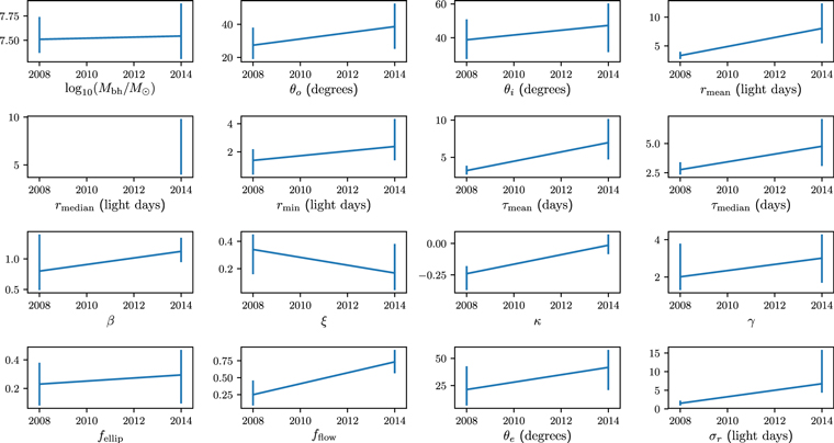
Figure 18. Change in the Hβ BLR model parameters from the LAMP 2008 campaign to the AGN STORM campaign. The vertical bars indicate the posterior PDF median and 68% confidence intervals for the two campaigns. The value of rmedian is missing for the 2008 campaign since it was not reported by Pancoast et al. (2014b).
Download figure:
Standard image High-resolution imageOther parameters that changed from the 2008 campaign to the 2014 campaign were  and κ. The change in
  indicates a switch from net-inflowing gas to net-outflowing gas. If true, this could suggest a significant change in the kinematics of the BLR that might be connected with the increase in AGN luminosity. However, we should note that with
  degrees for the AGN STORM campaign, the outflowing particles could be on highly elliptical bound orbits rather than on pure radial outflowing trajectories. The parameter κ shows a preference for Hβ emission from BLR clouds back toward the ionizing source in the 2008 campaign, but indicates a preference for isotropic emission in this data set.
Reassuringly, the black hole mass, opening angle, and inclination angles all remain consistent for the two data sets, as we would not expect these to change on a six-year timescale. Additionally, ξ remains the same, indicating a mostly opaque mid-plane. The parameters γ and  were not well constrained in either the 2008 or 2014 campaign models. Finally, the β parameter of the Gamma distribution was poorly constrained with the 2008 campaign data but is better determined with the 2014 campaign data.
This comparison of modeling results of a single AGN over multiple campaigns represents the second of its nature, with the first being Arp 151, presented by Pancoast et al. (2018).
6.3. Comparison of the Three Line-emitting Regions
The AGN STORM data set is the first data set in which this modeling technique can be applied to multiple emission lines for the same AGN. This gives us a unique opportunity to examine how the structure and kinematics of the three line-emitting regions are the same and how they differ. In Figure 9, we compare the posterior PDFs for the three BLR models. Each model used the same UV light curve as the driving continuum.
Examining the differences in model parameters, we clearly see radial ionization stratification (see, e.g., the rmedian distributions). Additionally, the radial distribution of particles is significantly different, with the C iv and Lyα BLRs having β close to 2 while the Hβ BLR has β ∼ 1. This also becomes clear when we show possible geometries of the three BLRs plotted on top of each other in Figure 19. There is clear radial structure in the three line-emitting regions, with C iv and Lyα emission coming from a very localized portion of a shell, while the Hβ region is much more spread out in the radial direction. The models displayed in the figure show the C iv BLR with a smaller minimum radius than the Lyα BLR, but the ordering of these two lines is not well constrained by the posterior parameter distributions.
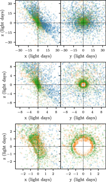
Figure 19. Possible geometries of the three line-emitting regions, with Hβ, C iv, and Lyα in blue, orange, and green, respectively. All panels show the same three geometries from different angles and different distance scales. Note that each model displayed is only one possible model from the posterior distribution, selected to have parameters closest to the median values reported in Table 1, and the exact radial ordering of C iv and Lyα is not constrained.
Download figure:
Standard image High-resolution imageWhile the rmin parameter is not well constrained for the Hβ versus UV models, the median value suggests that there is a ∼2.5 lt-day region between  and
and  in which there is Lyα emission but no Hβ emission. It is likely that there is still Hβ emission in this region, but in order to fit the stronger emission at larger wavelengths, the rmin parameter is shifted to larger radii. We discuss the possibility of tying the line emission to the underlying BLR gas distribution in Section 6.4.4.
The opening angle is surprisingly consistent between the three line-emitting regions. The inclination angle, on the other hand, shows some discrepancy. While it does not appear to be a huge difference, the discrepancy is at the  level, with
  (Hβ),
(Hβ),  (C iv),
  (Lyα). We examine this further in Section 5.2 and find that enforcing θi to be equal for all three regions leads to unphysical results in the radial ionization stratification of the BLR. Given that the Hβ BLR extends to a much larger radius than the C iv and Lyα BLRs, it is possible that they may lie at slightly different inclinations. For instance, a warped disk geometry would show a different inclination angle near the center than at larger radii. Since our model does not fit the underlying BLR gas, it is unclear whether the discrepancy arises from the gas distribution itself or is an effect only present in the gas emission.
6.4. Systematic Uncertainties and Model Limitations
6.4.1. A Simple Physical Model
When interpreting the results, it is important to keep in mind that we are using a simple model to describe what is likely a very complex region of gas. The current implementation of the code is not intended to explain the exact physical processes within the BLR, but rather to describe the overall size and shape of the BLR emission. It would be computationally infeasible to explore the parameter space of a full physical model of the BLR, so we neglect the details of, e.g., photoionization physics and radiation pressure and instead use a simple, flexible model that is designed to account for a wide range of possible BLR gometries and kinematics, while keeping the number of parameters and computational speed tractable. While these simplifications allow us to constrain the overall BLR structure and velocity field, there are certain details of the BLR that go un-modeled (see Raimundo et al. 2020, Section 2.2 for a discussion).
A blind test of reverberation mapping techniques found that for a mock data set, the inferred model parameters were in excellent agreement with the input BLR model, even though the details of the transfer function and rms profile were not fully captured (Mangham et al. 2019). Efforts are currently underway (P. R. Williams et al. 2020, in preparation) to include a more physically realistic description of the photoionization physics in the BLR. These additions to the model will provide the flexibility to fit more variability features in the emission line, and will naturally allow for effects such as “breathing” of the BLR.
6.4.2. Correlations among Model Parameters
With the high dimensionality of the BLR model parameterization comes a number of correlations between the model parameters. Grier et al. (2017) discuss in detail a degeneracy between the opening angle and inclination angle, pushing these two parameters toward similar values. In essence, in order to produce the single-peaked emission-line profiles we observe, θo ≳ θi, effectively putting a prior on the opening angle from θi to 90°. Therefore, it is possible that the BLRs actually have θo < θi, but have a structure and kinematics that cannot be reproduced by the current version of the model.
Additionally, given the parameterization of the model, there are multiple ways to combine model parameters to produce the same BLR model. For instance, as  , nearly all particles are placed in near-circular orbits, regardless of the value of
  or fflow. Similarly, a model with
  and
and  produces a line of particles perpendicular to the observer’s line of sight. However, this is equivalent to a face-on disk since rotations in the plane of the sky cannot be resolved with reverberation mapping data. These situations can increase the uncertainty on individual model parameters even if the particle distributions are very well determined.
6.4.3. Emission-line Model
When modeling a BLR, we assume that we can accurately isolate the broad emission line from contaminant features in the region of the line. If the contaminants are left in, the model will try to compensate by adjusting the parameters to fit this extra emission. Williams et al. (2018) show that the choices made when modeling an emission line, such as choice of Fe ii template, may influence the line profile enough to have an effect on the resulting model parameters. Pei et al. (2017) discuss the issues in decomposing the optical spectra for NGC 5548, including degeneracies between weak Fe ii and the continuum light as well as weak He i emission blended with Hβ. Similarly, the Lyα and C iv raw spectra have significant amounts of broad and narrow absorption which must first be modeled, making our resulting BLR models inherently dependent on the emission-line models.
6.4.4. Underlying BLR Gas
It is important to understand that the model use in this work is fitting the BLR gas emission and not the gas itself. There is, of course, gas elsewhere in the BLR that we do not see either because it is not emitting or because the emission is obscured. For instance, the fact that we see Lyα emission within  shows that emitting hydrogen gas is present in this region, yet we are unable to detect sufficiently strong Hβ emission.
Given a distribution of gas around the central BH and an ionizing spectrum, photoionization calculations are able to predict line emissivities through the BLR. Future dynamical modeling implementations can use these calculations to determine the distribution and motions of the underlying gas in the BLR, as well as the line emission. This will help shed light on some of the effects we see, such as the different inclination angles for C iv, Lyα, and Hβ emission.
Although the model used here does not have these features, its current aim is not to provide a full physical description of the BLR. Rather, we wish to describe the overall structure and motions of the BLR emission, and use this as a tool to measure black hole masses. Despite its limitations, the simple model achieves these goals, as evidenced by the consistent black hole mass measurements, agreement with cross-correlation lag measurements, and similar geometries to those inferred from the velocity−delay maps of Horne et al. (2020).
7. Summary
We have fit dynamical models of the BLR to three emission lines using the AGN STORM data set. This is the first time the modeling approach has been used to fit multiple emission lines for the same AGN, and is the first time it has been used with UV emission lines. Additionally, we fit the Hβ emission-line time series using both the UV light curve and V-band light curve as the driving continuum. This has allowed us to better understand the systematics involved in other modeling results when only the optical continuum is available (e.g., ground-based campaigns).
The main results of our analysis can be summarized as follows.
- 1.Modeling of Hβ, C iv, and Lyα provides three independent black hole mass measurements that are in good agreement. A joint inference combining all three lines gives
 . This is consistent with cross-correlation- and MEMEcho-based measurements with these data.
 - 2.
- 3.The different line-emitting regions do not need to lie in the same inclination plane. In NGC 5548, the C iv and Lyα BLRs share the same inclination angle, while the more extended Hβ BLR lies at a slightly higher inclination.
- 4.When the optical light curve is used as the driving continuum, the model parameters describing the Hβ BLR size (rmean, rmedian, rmin) are smaller by an amount comparable to the UV−optical lag, as opposed to when the UV light curve is used, and the black hole mass is under-estimated by a factor of τV/τUV. The parameters describing the BLR geometry and kinematics, however, are not significantly affected. This indicates that the V-band continuum is a suitable proxy for the ionizing continuum when studying the BLR structure and kinematics, but the UV−optical lag must be considered when measuring the BLR size.
- 5.The radius of the Hβ-emitting BLR increased by a factor of ∼3 between the 2008 LAMP campaign and the 2014 AGN STORM campaign, but the measured black hole mass remained constant. The other geometric parameters remained consistent in this time frame. There may have been a change in the BLR kinematics from inflow to outflow, although this is not robustly determined.
With the exquisite data analyzed in this paper, we have challenged the modeling method to recover the same black hole mass given three sets of data and to provide BLR properties using multiple light curves as the driving continuum. The consistent results have demonstrated that the modeling approach is a robust method of determining the BLR structural and kinematic properties, and reliable black hole mass measurements can be extracted from Lyα and C iv in addition to Hβ. Further, we have shown that the V-band continuum is a suitable proxy for the ionizing continuum for measuring BLR structural and kinematic properties, and reliable black hole mass estimates can be made provided the UV−optical lag is accounted for. The findings have provided insights into how the different line-emitting portions of the BLR fit together and how they evolve over time, and will help inform future improvements to the BLR model.
Support for HST program No. GO-13330 was provided by NASA through a grant from the Space Telescope Science Institute, which is operated by the Association of Universities for Research in Astronomy, Inc., under NASA contract NAS5-26555. Research by P.R.W. and T.T. is supported by NSF grants AST-1412315 and AST-1907208. T.T. and P.R.W. acknowledge support from the Packard Foundation through a Packard Fellowship to T.T. Research by AJB was supported by NSF grant AST-1907290. G.F. and M.D. acknowledge support by NSF (1816537, 1910687), NASA (17-ATP17-0141, 19-ATP19-0188), and STScI (HST-AR-15018, HST-AR-14556). M.I. acknowledges the support form the NRF grant, No. 2020R1A2C3011091, funded by the Korea government (MSIT). M.V. gratefully acknowledges support from the Independent Research Fund Denmark via grant No. DFF 8021-00130. C.S.K. is supported by NSF grants AST-1908952 and AST-1814440. V.N.B. acknowledges assistance from a NASA grant associated with HST proposal GO 15215, a NASA ADAP grant (grant # 80NSSC19K1016) and a National Science Foundation (NSF) Research at Undergraduate Institutions (RUI) grant (AST-1909297). Note that findings and conclusions do not necessarily represent views of the NSF. D.J.S. acknowledges funding support from the Eberly Research Fellowship from The Pennsylvania State University Eberly College of Science. The Center for Exoplanets and Habitable Worlds is supported by the Pennsylvania State University, the Eberly College of Science, and the Pennsylvania Space Grant Consortium. A.V.F.'s group at U.C. Berkeley is grateful for the financial support of NSF grant AST-1211916, the TABASGO Foundation, the Christopher R. Redlich Fund, and the Miller Institute for Basic Research in Science (U.C. Berkeley). Research at Lick Observatory is partially supported by a generous gift from Google.