Abstract
We present photometric and spectroscopic observations of the nearby (D ≈ 28 Mpc) interacting supernova (SN) 2019esa, discovered within hours of explosion and serendipitously observed by the Transiting Exoplanet Survey Satellite (TESS). Early, high-cadence light curves from both TESS and the DLT40 survey tightly constrain the time of explosion, and show a 30 day rise to maximum light followed by a near-constant linear decline in luminosity. Optical spectroscopy over the first 40 days revealed a reddened object with narrow Balmer emission lines seen in Type IIn SNe. The slow rise to maximum in the optical light curve combined with the lack of broad Hα emission suggest the presence of very optically thick and close circumstellar material (CSM) that quickly decelerated the SN ejecta. This CSM was likely created from a massive star progenitor with an  ∼ 0.2 M☉ yr−1 lost in a previous eruptive episode 3–4 yr before eruption, similar to giant eruptions of luminous blue variable stars. At late times, strong intermediate-width Ca ii, Fe i, and Fe ii lines are seen in the optical spectra, identical to those seen in the superluminous interacting SN 2006gy. The strong CSM interaction masks the underlying explosion mechanism in SN 2019esa, but the combination of the luminosity, strength of the Hα lines, and mass-loss rate of the progenitor seem to be inconsistent with a Type Ia CSM model and instead point to a core-collapse origin.
Original content from this work may be used under the terms of the Creative Commons Attribution 4.0 licence. Any further distribution of this work must maintain attribution to the author(s) and the title of the work, journal citation and DOI.
1. Introduction
Core-collapse supernovae (CCSNe) represent the end of the evolution of massive stars (≳8 M☉). Those supernovae (SNe) that exhibit hydrogen emission lines in their spectra are typically classified as Type II SNe, with further sub-type classifications depending on either their light-curve shapes (Type II-L, Type II-P) or spectroscopic signatures (Type IIn, Type IIb); see Arcavi (2017), Gal-Yam (2017), Branch & Wheeler (2017), Smith (2017) for detailed reviews. The class of CCSNe that show narrow or intermediate-width hydrogen emission lines in their spectra produced from the interaction between the SN ejecta and the surrounding circumstellar material (CSM) are classified as Type IIn (Schlegel 1990, where the “n” stands for narrow). In these systems, the narrow lines (∼102 km s−1) are formed from the ionization of the slow-moving CSM, while intermediate-width lines of a few 103 km s−1 arise from the interaction of the fast SN shock and the CSM. In many instances, broad 104 km s−1 emission is also seen, tracing the freely expanding SN ejecta. The ejecta-CSM interaction can create interesting multi-component emission lines that change as the SN evolves (e.g., Leonard et al. 2000; Trundle et al. 2009; Stritzinger et al. 2012; Smith et al. 2015; Andrews et al. 2017).
Type IIn SNe represent a diverse class of objects, and may come from various progenitor systems. Absolute magnitudes can range as high as –22 mag, as was seen in the superluminous IIn SN 2006gy (Ofek et al. 2007; Smith et al. 2007), although they generally reach a maximum brightness of –17 to –19 mag (Taddia et al. 2013). This makes SNe IIn brighter than most other CCSNe, owing to the kinetic energy of the SN explosion being converted to thermal energy through shock interaction. The progenitors of these SNe IIn are likely special cases of evolved massive stars with pre-SN outbursts, and could include extreme red supergiants (RSGs), yellow hypergiants (YHGs), or luminous blue variables (LBVs; Smith 2014).
The timescale of interaction can be fleeting or long-lasting depending on the radial extent and density of the CSM, which is a direct product of the mass-loss history of the progenitor. Estimates for CSM masses of most SNe IIn can range anywhere from 0.1 to 20 M☉ with mass-loss rates of 10−4 to 1 M☉ yr−1 (Smith et al. 2007; Kiewe et al. 2012). The CSM interaction not only affects the spectroscopic evolution but also the light-curve evolution, with rise times to maximum ranging from 14 to 61 days (Nyholm et al. 2020). Some objects even have flat late-time light curves that maintain brightness for decades after eruption (Turatto et al. 1993; Smith et al. 2017; Fox et al. 2020, e.g., SN 1988Z and SN 2005ip). For a full review of interacting SNe see Smith (2017).
Because a determining property of SNe IIn is nearby CSM creating narrow emission lines, thermonuclear SNe Ia can also create IIn observational signatures if they are surrounded by dense H-rich shells. Often referred to as Ia-CSM (or IIn/Ia), these objects show suggestive evidence of underlying SN Ia spectra, such as broad Fe and Si absorption lines diluted by excess continuum luminosity, as well as narrow hydrogen emission, and are often brighter than their normal SN Ia counterparts (Hamuy et al. 2003; Aldering et al. 2006; Silverman et al. 2013a; Leloudas et al. 2015). While many SNe IIn have been posited to actually be SNe Ia-CSM, only a handful show unambiguous evidence for SN Ia features due to the strength of the CSM interaction generally hiding the underlying Ia spectra. The best clear-cut case is that of PTF11kx, which showed late-onset interaction (Dilday et al. 2012; Silverman et al. 2013b), but the list of potential SN Ia-CSM is growing (Kotak et al. 2004; Trundle et al. 2008; Taddia et al. 2012; Fox et al. 2015a; Inserra et al. 2016; Graham et al. 2019). However, claims that these events actually arise from a thermonuclear SN Ia explosion have been controversial in several cases, because SNe Ic can have a similar spectral appearance at some phases, especially when diluted by CSM interaction (Benetti et al. 2006).
Often, nonterminal events such as luminous red novae (LRNe) or LBV outbursts are classified as Type IIn events because of the narrow Hα component (Ransome et al. 2021). Referred to as “SN imposters” (Van Dyk et al. 2000; Smith et al. 2011; Kochanek et al. 2012; Van Dyk & Matheson 2012; Pastorello et al. 2019), their fainter absolute magnitudes at maximum light, − 10 < MV < − 15 mag, generally differentiate them from terminal IIn events. In some cases the line between true SN and SN imposter is blurred. For instance, the terminal nature of both SN 2009ip and SN 2015bh is still debated (Fraser et al. 2013; Smith et al. 2016; Elias-Rosa et al. 2016; Thöne et al. 2017; Smith et al. 2022).
The optically thick CSM interaction zone in these objects masks the underlying ejecta, making it difficult to determine the type of explosion, whether it be core collapse, thermonuclear, or even a nonterminal eruption. One such object that falls into this category is the nearby SN 2019esa (Figure 1), which was discovered in ESO 035- G 018 at an R.A.(2000) = 07h55m00s.95, Dec.(2000)  during the course of the DLT40 one-day cadence SN search (for a description of the survey, see Tartaglia et al. 2018) on 2019 May 06 (Sand et al. 2019, MJD 58609.154). This object was given the designation DLT19c by the DLT40 team, but we use the IAU naming convention and refer to it as SN 2019esa throughout this work. The discovery magnitude was r = 17.2 mag, or Mr
≈ −15.0 mag, given the distance modulus we adopt below, which is at the transition from SN imposter to real SN. Within a day of discovery it was classified as IIn due to the prominent narrow Balmer emission lines (Uddin et al. 2019; Hiramatsu et al. 2019), and over the next month it rose to a maximum r = 14.5 mag, or Mr
≈ −17.7 mag, moving it into the regime of SNe IIn and not imposters. SN 2019esa was in the Transiting Exoplanet Survey Satellite (TESS) footprint, constraining the explosion date to MJD 58608.44 (Vallely et al. 2021, 2019 May 5.94), a value we adopt throughout the present paper.
during the course of the DLT40 one-day cadence SN search (for a description of the survey, see Tartaglia et al. 2018) on 2019 May 06 (Sand et al. 2019, MJD 58609.154). This object was given the designation DLT19c by the DLT40 team, but we use the IAU naming convention and refer to it as SN 2019esa throughout this work. The discovery magnitude was r = 17.2 mag, or Mr
≈ −15.0 mag, given the distance modulus we adopt below, which is at the transition from SN imposter to real SN. Within a day of discovery it was classified as IIn due to the prominent narrow Balmer emission lines (Uddin et al. 2019; Hiramatsu et al. 2019), and over the next month it rose to a maximum r = 14.5 mag, or Mr
≈ −17.7 mag, moving it into the regime of SNe IIn and not imposters. SN 2019esa was in the Transiting Exoplanet Survey Satellite (TESS) footprint, constraining the explosion date to MJD 58608.44 (Vallely et al. 2021, 2019 May 5.94), a value we adopt throughout the present paper.
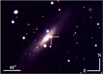
Figure 1. Composite gri Las Cumbres Observatory Siding Springs image of SN 2019esa taken on 2019 May 8.
Download figure:
Standard image High-resolution imageThe NASA/IPAC Extragalactic Database (NED) lists the heliocentric redshift of ESO 035–G018 as z = 0.00589. The most recent Tully-Fisher distance modulus value is μ = 32.22 ± 0.15 mag (Tully et al. 2016). Using H0 = 75.0 km s−1 Mpc−1 gives us a distance of  Mpc, a value we use throughout this paper. We do note the large range of redshift-independent distances to this galaxy (21.0 Mpc < D < 32 Mpc) listed in NED, which add uncertainties to the distance-calibrated measurements. This paper is structured as follows: in Section 2 observations and data reduction are outlined. We discuss the photometric and bolometric evolution in Section 3, and Section 4 details the spectroscopic evolution of the object. In Section 5 we lay out the implications of the observational data, and finally the results are summarized in Section 6.
2. Observations and Data Reduction
2.1. Imaging
Continuous photometric monitoring of SN 2019esa was done by the two discovery telescopes of the DLT40 survey, the PROMPT5 0.4 m telescope at Cerro Tololo International Observatory, and the PROMPT-MO 0.4 m telescope at Meckering Observatory in Australia, operated by the Skynet telescope network (Reichart et al. 2005). The PROMPT5 telescope has no filter (“Open”) while the PROMPT-MO telescope has a broadband “Clear” filter, both of which we calibrate to the Sloan Digital Sky Survey r band (see Tartaglia et al. 2018, for further reduction details). The sky location of SN 2019esa is located sufficiently close to the South Pole that it is circumpolar, and by keeping loose hour-angle constraints we were able to continuously observe the SN even when it was difficult with other facilities. The last nondetection from DLT40 was two days before discovery, on 2019 May 04 (JD 2458607.58), or 31 hr before the estimated explosion to a limiting magnitude of 19.2, and the first DLT40 detection was roughly 17 hr after explosion.
A high-cadence photometric campaign by the Las Cumbres Observatory telescope network (Brown et al. 2013) began immediately after discovery, in the UBVgri bands with the Sinistro cameras on the 1 m telescopes, through the Global Supernova Project. Using lcogtsnpipe (Valenti et al. 2016), a PyRAF-based photometric reduction pipeline, PSF fitting was performed. UBV-band data were calibrated to Vega magnitudes (Stetson 2000) using standard fields observed on the same night by the same telescope. Finally, gri-band data were calibrated to AB magnitudes using the Sloan Digital Sky Survey (SDSS, SDSS Collaboration et al. 2017). The light curves are shown in Figure 2.
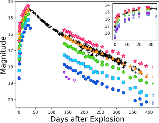
Figure 2. Optical photometry of SN 2019esa. The DLT40 r data are shown as black plus symbols and the marker size is larger than uncertainties for all data. The adopted date of explosion is MJD 58608.44 (2019 May 5.94). The inset shows a zoomed-in region of the first 35 days. The data set can be retrieved as the data behind the figure.(The data used to create this figure are available.)
Download figure:
Standard image High-resolution imageSN 2019esa was also observed by TESS (Ricker et al. 2015) during Sector 11, 12, and 13 operations of the mission, from 2019 April 23 07:02:56.026 to 2019 July 17 20:01:19.027 UTC. The TESS light curve of SN 2019esa was previously published in Vallely et al. (2021), and we present it here as well. In order to reduce the inherent scatter, the data have been binned into six-hour periods, beginning at the start of data acquisition. Where continuous monitoring was interrupted, the next six-hour bin began when observations resumed. Bins with less than five data points were removed. Compromised epochs, as determined by Vallely et al. (2021), were excluded from this process. The median flux, maximum flux error, and the mean observation time of the six-hour bin are shown in Figure 3 plotted against the DLT40 photometry. Both data sets have been normalized to the maximum magnitude for ease of comparison. The deviation in the light curves after maximum between DLT40 and TESS is likely due to the redder transmission curve of the TESS filter.
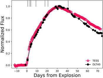
Figure 3. TESS and DLT40 light curves of SN 2019esa normalized to maximum light. TESS points are six-hour medians, and the JD of explosion is taken to be 2458608.94. The last nondetection from DLT40 (JD 2458607.65) is shown as a black triangle, and epochs of FLOYDS spectroscopy are indicated at the top of the plot by gray lines.
Download figure:
Standard image High-resolution image2.2. Spectroscopy
The majority of optical spectra were taken with the robotic FLOYDS spectrograph on the 2 m Faulkes Telescope South in Siding Springs, Australia, through the Global Supernova Project (FTS; Brown et al. 2013). A 2″ slit was placed on the target at the parallactic angle. One-dimensional spectra were extracted, reduced, and calibrated following standard procedures using the FLOYDS pipeline (Valenti et al. 2014), and are shown in Figure 4.
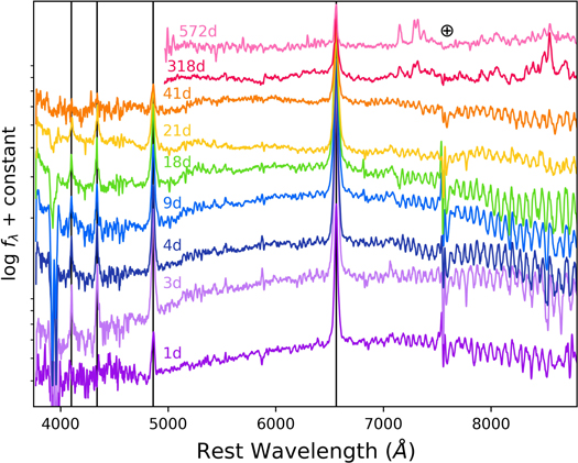
Figure 4. Optical spectroscopic evolution of SN 2019esa listed in Table 1. The rest wavelengths of the hydrogen Balmer lines are indicated by vertical black line. The spectra have not been corrected for reddening, and note that the epochs are measured from the estimated date of explosion, not from maximum light.(The data used to create this figure are available.)
Download figure:
Standard image High-resolution imageOne late-time spectrum was obtained with the Low Dispersion Survey Spectrograph 3 (LDSS-3) on the 6.5 m Magellan Clay telescope at Las Campanas Observatory in Chile. Standard reductions were carried out using iraf, including bias subtraction, flat-fielding, cosmic-ray rejection, local sky subtraction, and extraction of one-dimensional spectra. The slit was aligned along the parallactic angle to minimize differential light losses, and flux calibration was done using a spectrophotometric standard taken that night at similar airmass. A log of the spectroscopic observations shown in Figure 4 can be found in Table 1.
Table 1. Optical Spectroscopy of SN 2019esa
| UT Date | MJD | Phase | Telescope+ | R | Exposure Time |
|---|---|---|---|---|---|
| (y-m-d) | (days) | Instrument | λ/Δλ | (s) | |
| 2019-05-06 | 58609.38 | 1 | FTS+FLOYDS | 400 | 2700 |
| 2019-05-08 | 58611.45 | 3 | FTS+FLOYDS | 400 | 2700 |
| 2019-05-09 | 58612.39 | 4 | FTS+FLOYDS | 400 | 2700 |
| 2019-05-14 | 58617.43 | 9 | FTS+FLOYDS | 400 | 2700 |
| 2019-05-23 | 58626.37 | 18 | FTS+FLOYDS | 400 | 2700 |
| 2019-05-26 | 58629.35 | 21 | FTS+FLOYDS | 400 | 1800 |
| 2019-06-15 | 58649.34 | 41 | FTS+FLOYDS | 400 | 1800 |
| 2020-03-18 | 58926.45 | 318 | FTS+FLOYDS | 400 | 3600 |
| 2020-11-26 | 59180.26 | 572 | Magellan+LDSS3 | 750 | 1500 |
Note. Phases are reported with respect to an explosion epoch of MJD 58608.44.
Download table as: ASCIITypeset image
3. Light-Curve Analysis
3.1. Reddening Estimation
The Milky Way line-of-sight reddening for ESO 035- G 018 is E(B − V)MW = 0.16 mag (Schlafly & Finkbeiner 2011). While Na i D λλ5889,5896 Å absorption does appear to be present at the rest wavelength of the SN in at least some of the early spectra, indicating the presence of additional extinction, the low resolution of the FLOYDS spectra make it difficult to measure an accurate equivalent width (EW) to be used along with the prescription of Poznanski et al. (2012) to estimate the total reddening. The use of low-resolution spectra to determine a correlation between Na ID and extinction is discouraged in Poznanski et al. (2011) and Phillips et al. (2013), specifically in SNe. Furthermore, while Na i D can be an accurate tracer for cold interstellar dust along the line of sight, it is less reliable in the presence of hot circumstellar dust which we likely have around SN 2019esa. While we cannot use the Na i D absorption lines to estimate additional reddening, from the early spectra it appears that the SN is considerably reddened, likely from CSM dust. Therefore, we use comparisons with other well-studied SNe IIn in order to estimate the amount of total extinction toward SN 2019esa.
One way to estimate the reddening is by comparing the slope of the continuum to other IIn SN with low reddening at similar phases. The best candidates for this are SN 2009ip (Smith et al. 2010b, E(B − V) = 0.019) and SN 2010jl (Jencson et al. 2016, E(B − V) = 0.024). When we compare the SN 2019esa spectra near maximum (day 21 and 41) with the spectra of the other two SNe at maximum, our best-fit reddening occurs for E(B − V)tot = 0.52, or an E(B − V)host = 0.36. This value places the B − V color and absolute r magnitude of SN 2019esa comfortably within the ranges of other interacting SNe (Figure 5).
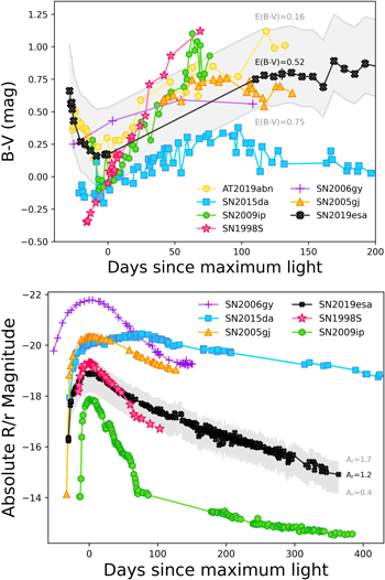
Figure 5. B − V color evolution (top) and absolute r/R mag light curves (bottom) of SN 2019esa compared with other interacting SNe. The black curve shows our adopted reddening of E(B − V) = 0.52 mag, but the full uncertainty range between the MW only reddening and E(B − V) = 0.75 mag is shown for SN 2019esa shaded in gray. We show data for SN 1998S from Liu et al. (2000), SN 2005gj from Prieto et al. (2007) and Krisciunas et al. (2017), SN 2009ip from Pastorello et al. (2013), SN 2006gy from Smith et al. (2007) and Agnoletto et al. (2009), SN 2015 da from Tartaglia et al. (2020), and AT2019abn from Williams et al. (2020). SN 2015 da has been shifted so that the initial rise matches that of SN 2019esa instead of the absolute maximum which was ∼100 days after explosion.
Download figure:
Standard image High-resolution imageThe top panel of Figure 5 shows the B − V color evolution of SN 2019esa along with a sample of other SNe IIn, which have been dereddened according to the published values. These include SN 2009ip (Pastorello et al. 2013), SN 1998S (Liu et al. 2000), and SN 2015 da (Tartaglia et al. 2020). Using the B − V color at maximum brightness, we find that an E(B − V)tot =0.75 (E(B − V)host = 0.59) for SN 2019esa gives the best color match with SN 2009ip, SN 1998S, and SN 2015 da. Converting this E(B − V) value to an extinction using Fitzpatrick (1999), we obtain an Ar = 1.71 mag.
We can also attempt to use the Balmer decrement to get a rough estimate of the total reddening toward SN 2019esa. This is not exactly a reliable method, as we expect the interaction to help produce different intrinsic Hα/Hβ ratios, but it may help to provide approximate limits. For Case B recombination, we would expect a ratio to Hα/Hβ of 2.87 for a T = 10,000 K (Osterbrock & Ferland 2006). We must point out that the ratio changes with time as the SN reaches maximum (Table 2). This could be due in part to the low signal-to-noise ratio (S/N) in the blue end around Hβ of a few epochs introducing larger uncertainties, but it could also indicate changing conditions in the SN environment. For instance, the Balmer decrements of SN 2009ip and SN 2015bh dropped from values well above Case B to near unity as the SN reached maximum light, and then rose again afterward (Levesque et al. 2014; Thöne et al. 2017). The low values of the Balmer decrement in these cases were attributed to themalized emission in an ejecta with densities of ne > 1013 cm−3 during the peak luminosity. If we measure the integrated flux of both lines from spectra that have been corrected for only E(B − V)MW = 0.16, we find that for days 3, 4, and 9 (which have the highest blue-end S/N) the average total reddening needed is E(B − V) = 0.55, a value consistent with the one obtained by comparing continuum slopes to SN 2009ip and SN 2010jl.
Table 2. Balmer Line Properties for E(B − V) = 0.52 mag
| Age | Hαa | Hβ | Hα/Hβ | ||||
|---|---|---|---|---|---|---|---|
| days b | FWHM | Flux | Log(L) | FWHM | Flux | Log(L) | |
| 1 | 1020 | 2.3 | 40.32 | 1600 | 0.6 | 39.77 | 3.6 |
| 3 | 1100 | 8.9 | 40.92 | 1450 | 3.2 | 40.47 | 2.8 |
| 4 | 1115 | 10.1 | 41.00 | 1515 | 3.8 | 40.54 | 2.9 |
| 9 | 1190 | 17.3 | 41.21 | 1575 | 5.6 | 40.72 | 3.1 |
| 18 | 1200 | 18.3 | 41.23 | 1610 | 7.8 | 40.86 | 2.3 |
| 21 | 1200 | 15.7 | 41.16 | 1840 | 9.0 | 40.92 | 1.7 |
| 41 | 1295 | 13.4 | 41.10 | 1960 | 5.5 | 40.71 | 2.4 |
| 318 | 1320 | 1.9 | 40.26 | ⋯ | ⋯ | ⋯ | ⋯ |
| 572 | 900 c | 0.003 | 37.38 | ⋯ | ⋯ | ⋯ | ⋯ |
Notes.
a Full width at half maximum (FWHM) units are km s−1, flux units are in 10−13 erg s−1 cm2, and luminosity units are in erg s−1. b With respect to explosion epoch of MJD 58608.44. c Gaussian.Download table as: ASCIITypeset image
Due to the uncertainties in the reddening, we take E(B − V)tot = 0.52 mag as the most likely value, with the uncertainties spanning the ranges of no additional reddening (MW only) and the largest value obtained from matching the B − V color at maximum (E(B − V)tot = 0.75 mag). Therefore, a value of  mag is used throughout this paper. The full range of light and color curves with this reddening applied is shown as gray shaded regions in Figure 5.
3.2. Light-Curve Evolution
The full photometric evolution of SN 2019esa can be seen in Figure 2, including the high-cadence DLT40 r-band data. Following Vallely et al. (2021), who use a curved power law (see their Equation 2.) to fit the TESS data, we use an explosion epoch of MJD 58608.44. Both the DLT40 and TESS photometry indicate a date of maximum light of around MJD 58640, or roughly 32 days to a maximum r = 14.51 mag. There is a break in the multi-band Las Cumbres Observatory coverage right around maximum light due to hour-angle constraints, but the B-band data also show a maximum around MJD 58636, or 28 days post explosion. For comparison, typical rise times for noninteracting Type II SNe are around 10 days in r-band (González-Gaitán et al. 2015), and roughly 19 days for a SN Ia (Firth et al. 2015). Introducing CSM interaction can lengthen the rise time depending on the radial density structure of the CSM, potentially increasing it to weeks or months in SNe IIn (Nyholm et al. 2020) and Ia-CSM (Silverman et al. 2013a).
The relaxed hour-angle constraints of the DLT40 monitoring allowed for continuous coverage out to roughly 400 days post explosion. The resulting light curve shows an almost linear decline of 4 mag from maximum until our final observation, or a rate of ∼0.011 mag day−1. When Las Cumbres Observatory began observing again on MJD 58748, the BgVi data all show a slightly slower decline rate of ∼0.009 mag day−1, while the Las Cumbres Observatory r is similar to that of DLT40 at ∼0.010 mag day−1. This value is almost identical to that of the interacting (and possible Ia-CSM) SN 2005gj (Prieto et al. 2007), and similar to other values measured in other interacting SNe (Kiewe et al. 2012; Kilpatrick et al. 2016, for example), although we expect a wide range of decline rates as the CSM around interacting SNe will have different densities and geometries.
The bottom panel of Figure 5 shows the absolute r magnitude light curve of SN 2019esa compared to the r/R band light curves of other SNe IIn and Ia-CSM/IIn. All SNe have been dereddened by values listed in the literature. Because of the uncertainty in the reddening of SN 2019esa, we show the light curve corrected for Ar = 1.2 mag, as well as the extinction uncertainty range shown in the shaded region. This puts the range of absolute magnitude at maximum in the range –18.1 < Mr < –19.4 mag. These are quite similar to the max Mr for IIn SNe SN 2009ip and SN 1998S, but significantly fainter than the IIn SN 2015 da and the superluminous supernova (SLSN) SN 2006gy. We note that when we deredden the spectra of SN 2019esa so that the absolute magnitude at peak matches that of SN 2006gy (Ar = 4.1 mag) the spectral energy distribution (SED) of SN 2019esa becomes too blue to be physically possible.
While the absolute magnitude at maximum of SN 2019esa may be similar to those of SN 2009ip and SN 1998S, the rise time is significantly slower. Comparatively, the ∼30 day rise to maximum is much shorter than the rise time for SN 2006gy which took about 70 days to reach an absolute magnitude of −21 (Smith et al. 2007), or the IIn SN 2015 da which had a very quick rise in brightness but then took around 100 days to reach the absolute maximum (Tartaglia et al. 2020). The potential Ia-CSM SN 2005gj r-band rise was almost identical to SN 2019esa at 31.7 days (Prieto et al. 2007), although the bluer bands of SN 2005gj rose much faster (12.7 days in u, 18.5 in g), while all optical colors of SN 2019esa appear to have similar ∼30 day rises.
3.3. Color, Temperature, and Radius Evolution
Unlike most IIn SNe, SN 2019esa has an unusual color evolution (top panel, Figure 5) where it becomes bluer as the light curve rises to peak, then slowly reddens after max brightness. While uncommon for most CCSNe, this behavior has been seen to varying amounts in the IIn SN 1988Z (Turatto et al. 1993), SN 2006aa (Taddia et al. 2013), and in SN 2009ip (Fraser et al. 2013; Graham et al. 2014). It has also been noted in the ILRT objects AT 2017be (Cai et al. 2018), SNHunt120 (Stritzinger et al. 2020), and AT 2019abn (Jencson et al. 2019). In the case of AT 2019abn, the detection of F-type absorption features in multiple spectra during the rise indicated a constant photospheric temperature of ≈7000–8000 K. This lead Jencson et al. (2019) to suggest that the early evolution to bluer colors was due to continuous dust destruction in the CSM surrounding the star. It is plausible that a similar effect could be at least partly responsible for the odd color evolution in SN 2019esa, though we do not have direct evidence of this.
Figure 6 shows a quasi-bolometric light curve of SN 2019esa created using the Light Curve Fitting package from Hosseinzadeh & Gomez (2020). Similarly to what was done in Hosseinzadeh et al. (2022), a blackbody spectrum was fit to the SED at each epoch, and the resulting best-fit blackbody was integrated over the available bands to create a pseudobolometric light curve. The resultant temperature and radius from the SED fits are also shown in Figure 7. The data have been corrected for an E(B − V)tot = 0.52 mag and the adopted distance modulus μ = 32.22 mag. The blackbody-corrected bolometric light curve is shown as black diamonds, with the range from reddening uncertainties shown in gray. We also plot the DLT40 open-filter light curve in blue—shifted to match the late-time bolometric light curve—to show the likely shape of the Lbol during the gap in the Las Cumbres Observatory coverage. Integrating over the blackbody-corrected light curves for the first 400 days (using a straight-line interpolation over the gap) gives a total radiated energy of Erad ≈ 0.5 − 2.6 × 1050 ergs. This is likely a lower limit though, as no ultraviolet (UV) or infrared (IR) photometry was used in deriving the bolometric luminosity.
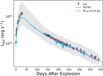
Figure 6. Pseudobolometric, blackbody-corrected light curve of SN 2019esa (black diamonds) constructed from the optical photometry and assuming an E(B − V) = 0.52 mag. The gray shaded region spans the possible reddening uncertainties. The 56Co decay rate for  = 0.55 M⊙ is indicated by the dashed magenta line. The DLT40 light curve is also shown shifted to match the late-time bolometric luminosity to show the possible light-curve evolution during the lack of Las Cumbres Observatory data.
Download figure:
Standard image High-resolution image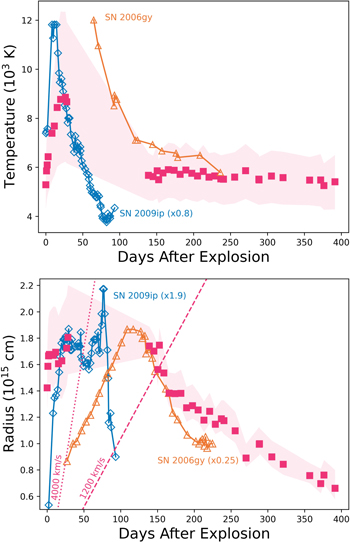
Figure 7. Blackbody temperature (top) and radius (bottom) evolution of SN 2019esa derived from the optical photometry shown by magenta squares. All data have been dereddened by our assumed E(B − V)tot = 0.52, with the uncertainties from the reddening indicated by the shaded regions. Data of SN 2006gy (Smith et al. 2010a) and SN 2009ip (Graham et al. 2014) are shown for comparison. Any scaling values are indicated. Additionally, lines of constant velocity of the full width zero intensity (FWZI; dotted) and FWHM (dashed) of Hα are shown in the bottom panel.
Download figure:
Standard image High-resolution imageFrom the bolometric light curve we can see that between days ∼125 and 250 the luminosity decline is similar to that of fully trapped 56Co decay of 0.98 mag 100 day−1, but may deviate by small amounts at later times. This luminosity can be produced by roughly  = 0.55 M☉ (magenta dashed line in Figure 6.) If we estimate the mass of 56Ni on day 139 using Lbol
we obtain a value of
= 0.55 M☉ (magenta dashed line in Figure 6.) If we estimate the mass of 56Ni on day 139 using Lbol
we obtain a value of  = 0.58 M☉, and on day 391
  = 0.67 M☉ (Pejcha & Prieto 2015). Of course, this may be an overestimate because the CSM interaction could still be strong and contributing to the late-time luminosity, although without adequate spectroscopic coverage during this time it is difficult to determine the amount of contribution. For comparison, normal Type II SNe have an average
  = 0.04 M☉ (Valenti et al. 2016; Müller et al. 2017; Rodríguez et al. 2021), and type Ia SNe 0.1 M☉ <
  < 1.1 M☉ (Cappellaro et al. 1997; Contardo et al. 2000; Stritzinger et al. 2006; Scalzo et al. 2019).
Just as in the color evolution of SN 2019esa, the evolution of TBB and RBB, shown in Figure 7, is somewhat unusual. Unlike most SN IIn, which have their highest temperature at explosion (or at least at discovery) and cool quickly with time (Taddia et al. 2013), TBB for SN 2019esa actually rises over the first ∼35 days from a relatively cool ∼5500 to ∼9000 K (or ∼12,000 K with our highest reddening). This temperature then drops at some point during our lack of multi-wavelength coverage, but then stays relatively constant at around 6000 K from day 125 until day 400. This low, late-time TBB of ∼6500 K is commonly seen in IIn SNe. The range in TBB seen in SN 2019esa is similar to the interacting SNe 2006gy, 2005gj, 1998S, and 2016aps (Fassia et al. 2000; Prieto et al. 2007; Smith et al. 2010a; Nicholl et al. 2020), although these objects do not show the 30-day temperature rise after explosion. SN 2009ip did show this temperature increase during the second outburst event in 2012 (Graham et al. 2014), and it is possible that SN 2006gy did increase in temperature, but data were not obtained at sufficiently early epochs. Both the TBB and RBB for SN 2006gy and SN 2009ip are shown in Figure 7, and come from Smith et al. (2010a) and Graham et al. (2014), respectively. This strange behavior can be understood by also looking at the color and spectral evolution. As the luminosity rises over the first few months, the flux rises more in the blue than in the red.
The evolution of the RBB of SN 2019esa rises to a maximum value somewhere between 50 and 150 days after explosion, only to fall again over the next 250 days. It is important to emphasize here that in SN IIn, RBB does not carry significant importance because the interaction often removes much of the physical meaning. The narrow range of RBB values between 0.6 and 1.8 × 1015 cm derived for SN 2019esa is consistent with other IIn SNe (Taddia et al. 2013), but smaller than the much brighter interacting SN 2006gy and SN 2005gj whose RBB had maximum values of 4 and 8 × 1015 cm, respectively (Prieto et al. 2007; Smith et al. 2010a), and almost twice as large as that for the hotter SN 2009ip (Graham et al. 2014). Interestingly, the peak of RBB between 50 and 150 days is consistent with the ∼50 days for SNe 1998S (Fassia et al. 2000) and 2005gj (Prieto et al. 2007) and the ∼115 days for SN 2006gy (Smith et al. 2010a). We also plot in the bottom panel of Figure 7 the constant velocity curves of material moving at 4000 km s−1 and 1200 km s−1, and the FWZI and the FWHM, respectively, of the Hα emission shown in Figure 8.
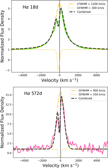
Figure 8. Hα emission line on day 18 (top) and 572 (bottom). Day 18 can be reproduced by a Lorentzian emission profile combined with a much narrower Gaussian absorption profile. This creates a P Cygni feature with a FWHM of 300 km s−1. Day 572 is better represented by a 900 km s−1 Gaussian emission profile combined with a 250 km s−1 absorption profile.
Download figure:
Standard image High-resolution imageWe note that the turnover in RBB occurs at roughly the intersection of a constant 1200 km s−1 velocity, the FWHM of the intermediate-width line. The epoch when RBB stops increasing, either by stalling at a constant value or even decreasing as we see here, may occur when the forward shock has finally traversed the majority of the CSM. Unfortunately, we have no optical spectra during this time to check for any obvious physical changes that would support this claim. If we assume that it does take 150 days to traverse the bulk of the CSM, at a velocity of 1200 km s−1, this suggests the circumstellar shell extends to about 1.5 × 1015 cm. If the surrounding CSM material is similar to that of SN 2006gy or SN 2006tf, RBB does not represent the true photospheric radius and the decrease in RBB may be due instead to the shell-covering factor decreasing as the optical depth drops (Smith & McCray 2007; Smith et al. 2008). In other words, the post-shock shell may be very clumpy, allowing regions of high optical depth dispersed within an optically thin medium (Chevalier & Fransson 1994).
4. Spectral Evolution
SN 2019esa shows spectroscopic characteristics typical of SN IIn, with strong, intermediate-width (∼1000 km s−1) Balmer emission. While normally early spectra of Type II SNe (interacting or not) show very blue continua that are either mostly featureless, or exhibit high-ionization emission lines such as N v λλ4434,4641, He ii λ4686, and C iv λλ5801,5812, SN 2019esa appears quite red with only strong hydrogen emission lines and deep Ca H & K absorption. A dense, hydrogen-rich CSM enshrouding the SN could act to dampen the strengths of any of the high-ionization features.
Over the first two weeks, the spectra do gradually become bluer as the luminosity and temperature continue to rise. The strong Balmer emission lines seen in the spectra can be easily fit by a single Lorentzian profile for all but the last epoch. In the last epoch, the Lorentzian profile has disappeared and Hα can best be fit by a Gaussian with a FWHM of 900 km s−1. Table 2 lists the measured FWHM, fluxes, and luminosities of Hα and Hβ only, but we note that the bluer Balmer emission lines show similar widths. The Lorentzian profile is likely caused by electron scattering in the optically thick CSM (Chugai 2001; Smith et al. 2008), and therefore the FWHM may be a slight overestimate of the true shock velocity if electron scattering is present in the wings of the lines. This seems to still be occurring as late as 318 days after explosion. Combining the persistence of electron scattering along with the roughly constant FWHM of the lines (Hα in particular) for the first year after explosion, it is clear that the CSM surrounding SN 2019esa must be extremely dense.
In the day 18 spectrum, which had the best seeing of all of the FLOYDS spectra, a narrow Hα absorption component is seen at −115 km s−1 (Figure 8, top). A similar feature is also seen at the same location in the higher resolution, day 572 LDSS3 spectrum (Figure 8, bottom). The absorption line is too close to Hα to be from over-subtraction of galactic [N ii] lines, and its appearance in two different epochs with two different instruments suggests that it is real. The FWHM of the absorption line ranges between 250 and 300 km s−1, velocities consistent with the winds of LBVs and BSGs, although the low resolution of the instruments cannot rule out slower RSG or YSG progenitor systems. The persistence of this narrow emission line in our last spectrum also suggests the existence of CSM that has yet to be traversed by the SN shock.
Unlike most interacting SNe, at no time do we see any underlying broad emission from the quickly expanding SN ejecta, the caveat being there are large gaps in the spectral coverage after the first two months, and in this gap during the decline from peak is when one would expect to see these broad lines appear. This indicates that the continuum emission coming from the CSM interaction is (at least at early times) producing a photosphere outside of the forward shock, prohibiting a glimpse into the internal SN ejecta. At late times when the CSM interaction region has expanded out to larger radii containing less dense pre-shock gas, it finally becomes optically thin, but the SN ejecta has faded significantly so that it becomes nondetectable over the much stronger CSM interaction.
In the last two epochs, it is clear that the spectra are still strongly dominated by CSM interaction, and lack some of the normal nebular emission lines that are usually present in typical CCSNe without CSM interaction, mainly O and He. The lack of [O i] is not surprising because it is rarely seen in interaction-powered SNe (Fox et al. 2015a), but He i is often seen in SNe IIn (e.g., SN 2009ip and SN 1998S, shown in Figure 9). It is likely that we are beginning to see some of the cool dense shell (CDS) due to the emergence of the emission lines of [Ca ii], the Ca ii IR triplet, and possibly a Paschen 10-3 line at 9017 Å. Most intriguing is the presence of possible neutral Fe lines, which we discuss in more detail below. Although there is significant blending, the widths of the lines are roughly 1000 km s−1, consistent with that of Hα. This suggests that these lines originate from the same location as the hydrogen lines, likely in the post-shock CDS.
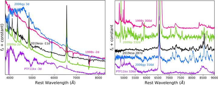
Figure 9. Left: Comparison of optical spectra of SN2019esa (black) with other IIn and Ia-CSM SNe near maximum light. Spectra have been corrected for reddening and come from Smith et al. (2007, SN 2006gy), Fassia et al. (2001, SN 1998S), Fraser et al. (2013, SN 2009ip), and Dilday et al. (2012, PTF11kx). The epoch with respect to maximum brightness is listed by the SN name. Right: Same as left panel, but at later times. Spectra are from Leonard et al. (2000, SN 1998S), Smith et al. (2014, SN 2009ip), Kawabata et al. (2009, SN 2006gy), and Silverman et al. (2013b, PTF11kx).
Download figure:
Standard image High-resolution image5. Discussion
5.1. Location and Size of the CSM
The fact that no broad ejecta lines are seen in our spectra, and the persistence of intermediate-width lines even in our earliest spectra, suggest that the CSM surrounding SN 2019esa is quite dense. Similar to the very luminous IIn SN 2006tf, it is likely that the SN shock is quickly decelerated by the massive CSM, preventing the fast ejecta expansion that gives rise to the broad emission lines, and instead converts the bulk of the kinetic energy into thermal energy and light (Smith et al. 2008), creating an extra energy source that increases the intrinsic brightness of the SN. This would also explain the slower (∼30 day) rise to maximum of the light curve as the energy deposited into the optically thick CSM would have to slowly diffuse out (Smith & McCray 2007). Additionally, the narrow P-Cgyni absorption is still seen in our last spectrum on day 572, indicating the continued presence of some slow, unshocked CSM, which would be at a radius of at least 6 × 1015 cm.
Although we do not have any X-ray or radio data of SN 2019esa, we can use the luminosity and kinematics of the system offered to us through our bolometric light curve and optical spectra to determine a wind-density parameter w and therefore a rough estimate of the mass-loss rate of the progenitor star. This can be expressed as  =
=  , where VCSM is the CSM velocity measured from the minimum of the narrow P Cygni lines and VSN is the SN expansion velocity (see Smith 2017). At early times, the speed of the shock is unknown because it is hidden below the photosphere, but from our day 318 spectrum, VSN = 1320 km s−1 (taken from the FWHM of Hα) and we assume VCSM = 300 km s−1 from our day 18 and day 572 spectra (although this is likely an upper limit). From our bolometric light curve, we measure L = 5.1 × 1041 erg s−1 on day 318, resulting in an
  = 0.2 M☉ yr−1 (or a range of 0.12–0.33 M☉ yr−1 using the full reddening uncertainty.) If we assume that the pre-SN mass loss occurred 3–4 yr prior (
 ), this would suggest a total mass loss of 0.5–1.5 M☉.
Mass-loss rates of a sample of IIn from Kiewe et al. (2012) range between 0.026 and 0.12 M☉ yr−1, and in particular  ∼2 × 10⁻⁵
M☉ yr−1 for SN 1998S (Fassia et al. 2001), and
∼2 × 10⁻⁵
M☉ yr−1 for SN 1998S (Fassia et al. 2001), and  ∼1–6 × 10⁻⁵
M☉ yr−1 for the interacting (and possible Ia-CSM) SN 2005gj (Trundle et al. 2008). The extremely long-lived IIn SN 2015 da did have a very high
∼1–6 × 10⁻⁵
M☉ yr−1 for the interacting (and possible Ia-CSM) SN 2005gj (Trundle et al. 2008). The extremely long-lived IIn SN 2015 da did have a very high  = 0.6–0.7 M☉ yr−1 (Tartaglia et al. 2020), while mass-loss rates of SN 2006gy range anywhere between 0.1 and 0.5 M☉ yr−1 (Smith et al. 2007; Moriya et al. 2013). The only progenitor channel capable of mass-loss rates on the order of 0.5 M☉ yr−1 would be from a prior eruption of an LBV, akin to the Great Eruption of η Car (Davidson & Humphreys 1997; Morris et al. 1999; Smith et al. 2003). The ∼1–2 M☉ of CSM we estimate for SN 2019esa could have been lost over a short amount of time during a similar eruptive event.
5.2. Comparison to SN 2006gy
SN 2006gy was a SLSN maintaining a magnitude of at least −21 mag for well over 100 days, with Type IIn spectra (Ofek et al. 2007; Smith et al. 2007; Agnoletto et al. 2009; Smith et al. 2010a). While SN 2019esa is less luminous, there are similarities between the optical spectra (Figure 10) and the shape of the light curve of the two objects that are worth exploring.
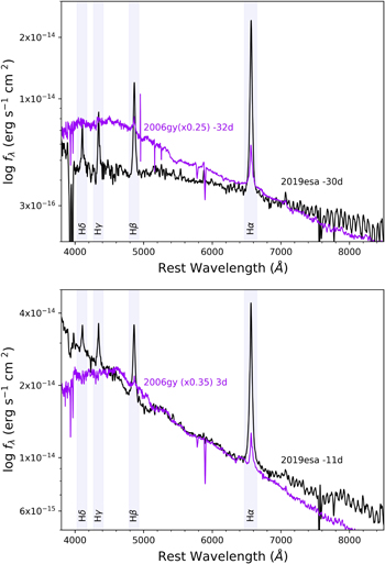
Figure 10. Spectral comparison between SN 2019esa and SN 2006gy before maximum (top) and near maximum (bottom). SN 2006gy spectra are from Smith et al. (2007). All spectra have been corrected for reddening and all epochs are with respect to the date of r/R-band maximum.
Download figure:
Standard image High-resolution imageThe lower panel of Figure 5 shows the absolute r/R-band light curves of both objects. The differences in peak magnitudes are easily seen, with the total radiated energy of SN 2006gy estimated to be ∼2 × 1051 ergs (Smith et al. 2010a), while SN 2019esa appears less energetic at ∼1 × 1050 ergs. The rise times are also noticeably different, with the substantially more luminous SN 2006gy taking roughly twice the amount of time as SN 2019esa to rise to maximum at ∼70 days (Smith et al. 2007). Various estimates from observations and models for SN 2006gy all require a high CSM mass of order 10–25 M⊙ (Smith et al. 2007; Smith & McCray 2007; Woosley et al. 2007; Smith et al. 2010a; Moriya et al. 2013). The SN ejecta mass must have at least a comparable mass in order to maintain the high observed speed of SN 2006gy’s CDS (Woosley et al. 2007; Smith et al. 2010a). A mass loss of such a high amount plus similarly massive ejecta requires an extremely massive progenitor star. A similar scenario with a less massive CSM of 1–2 M⊙ may be responsible for the observational characteristics of SN 2019esa.
At all comparable epochs, there is a lack of He i emission, unlike in some other IIn SNe (e.g., SN 2009ip shown in Figure 5), which is consistent with the low (< 12,000 K) temperatures of both objects. In the SN 2006gy spectrum taken at roughly 287 days after maximum, Hα is extremely weak while it appears to be quite strong in SN 2019esa around the same age. In fact, comparison of the Hα luminosities of SN 2006gy presented in Smith et al. (2010a) with those of SN 2019esa listed in Table 2 shows that the Hα brightness of SN 2019esa is roughly four times that of SN 2006gy at all comparable phases. Other than this one difference, it is these late-time spectra that show the most similarities between the two objects, specifically the intermediate-width, resolved Fe i, Fe ii, and Ca ii emission lines seen redward of Hα (Figure 11).
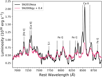
Figure 11. Spectral comparison between SN 2019esa (316 days post maximum) and SN 2006gy (287 days post maximum) in luminosity space. SN 2006gy spectra are from Kawabata et al. (2009). Both spectra have been dereddened and we have used the distance and reddening adopted for SN 2006gy from Jerkstrand et al. (2020). The line strengths are almost identical in both spectra except for the stronger Ca emission in SN 2019esa.
Download figure:
Standard image High-resolution imageThere has been some disagreement in the literature as to whether SN 2006gy was a core collapse or thermonuclear event, although there is consensus that interaction with massive CSM did occur. Late-time HST and Keck AO imaging eliminate the need for a pulsational pair instability model for the explosion of SN 2006gy after revealing the presence of IR and scattered-light echoes (Smith et al. 2008; Miller et al. 2010; Fox et al. 2015b), and an interaction-powered model with up to 10–25 M☉ of CSM is required to reproduce the high luminosity and long duration of the light curve (Smith et al. 2007; Smith & McCray 2007; Woosley et al. 2007; Agnoletto et al. 2009; Smith et al. 2010a; Moriya et al. 2013). More recently, though, Jerkstrand et al. (2020) analyzed the late-time spectra of SN 2006gy, and revived the idea first put forth in Ofek et al. (2007) that the event was a SN Ia occurring inside a dense CSM. In particular, this argument concentrated on the emission of neutral Fe lines in the late-time spectra, which those authors interpreted as being powered by radioactive decay in the nebular SN ejecta with a high Fe abundance. The striking similarities between the late-time spectra of SN 2019esa and SN 2006gy prompt us to question the hypothesis of a Type Ia-CSM for both SNe, and is discussed in the following section.
5.3. Core-collapse or Thermonuclear?
SN Ia-CSM is still a poorly understood observational class, owing to the strong CSM interaction which effectively obscures the underlying SN emission. The luminosity range for Ia-CSM is − 19.5 < MV < − 21.6 (Leloudas et al. 2015), and their optical spectra show Hα and weak Hβ emission lines with generally a lack of He i (Silverman et al. 2013a). More importantly, SNe Ia-CSM normally appear spectroscopically as diluted SNe Ia, then slowly begin to show narrow hydrogen emission lines that get stronger with time as the SN ejecta plows into the CSM. Only in those objects with weaker CSM interaction can the thermonuclear nature be confirmed, with PTF11kx (Figure 9) being the most unambiguous case of a SN Ia-CSM (Dilday et al. 2012; Silverman et al. 2013b; Graham et al. 2017).
For SN 2019esa, we can rule out the appearance of Ia-like spectra at early times because only narrow hydrogen emission lines are seen superimposed on a smooth blue continuum. Furthermore, the Hα luminosities for SN 2019esa (see Table 2) are much higher than the 1–9 × 1040 erg s−1 normally seen in Ia-CSM (Silverman et al. 2013a). This may be due to the stronger-than-normal CSM interaction obscuring the underlying thermonuclear explosion or could point to a core-collapse origin. Like Ia-CSM, SN 2019esa also lacks He emission lines, but this line is also missing in many core-collapse SNe IIn. Using an E(B − V) = 0.52 mag, the absolute magnitude of SN 2019esa rose to Mr = –18.9 mag, which is on the lowest end of typical peak luminosities of normal SNe Ia without CSM interaction. Combined with the lack of SN Ia features in the spectrum near peak, this makes a SN Ia-CSM model highly unlikely for SN 2019esa. Although we must reiterate that the extinction correction could be smaller, and the SN even less luminous, strengthening this argument. The CSM surrounding SN 2019esa is likely massive, and therefore the energetics of a normal SN Ia combined with the kinematics of CSM-shock interaction would have produced a much brighter transient than was observed. Additionally, the mass-loss rates estimated for SN 2019esa and needed to sustain the CSM interaction for well over a year are much too high for thermonuclear progenitors. For instance, the proposed SN Ia-CSM SN 2002ic had an estimated mass-loss rate of ∼10−4 M☉ yr−1 (Kotak et al. 2004), and SN 2008J was roughly 3 × 10⁻³ M☉ yr−1 (Taddia et al. 2012). However, Silverman et al. (2013a) estimate mass-loss rates from their sample of possible SNe Ia-CSM to be much larger at a few 10−1 M☉ yr−1 based on rise times and X-ray observations.
The late-time spectra may prove the best evidence we have of the true nature of SN 2019esa, in particular the presence of the [Ca ii] λλ7291, 7324 doublet, which is normally not seen in Ia-CSM (Silverman et al. 2013a). Additionally, the Ca ii triplet is broad and blended in SN Ia-CSM (e.g., PTF11kx in Figure 9), but in SN 2019esa the individual Ca ii components are easily resolved owing to the much lower line velocities. Most intriguing are the forest of Fe i and Fe ii emission lines (Figure 11), which, as we discuss below, have been proposed as additional evidence for a Ia-CSM nature in SN 2006gy, along with the extreme luminosity of the object. Other than these late-time Fe emission lines, there is no evidence that SN 2019esa is of a thermonuclear origin, and there is considerable reason to doubt such an association.
The argument for the Ia-CSM nature of SN 2006gy presented in Jerkstrand et al. (2020) hinges on the existence of these neutral Fe lines that emerge in the late-time spectra, combined with it is extreme luminosity, and the assertion that they must arise from Fe-rich nebular SN ejecta powered by radioactivity. From their analysis applying a nebular-phase SN Ia radiative transfer model, these authors suggest at least 0.3 M☉ of iron has been mixed with a 20 M☉ shell of H-rich CSM. It is this dense CSM that quickly decelerated the ejecta and trapped gamma-rays, giving rise to the intermediate-width Fe lines at later times. However, the ionization level and density used to derive this mass of Fe come from a nebular SN Ia model powered by radioactivity, even though the luminosity at late times in SN 2006gy is clearly decaying more slowly than for 56Co and is not powered by radioactivity (Smith et al. 2008; Miller et al. 2010; Fox et al. 2015b). It is also worth noting that strong Fe i and Fe ii lines are seen in the CSM shells of LBVs like η Car (Hartman et al. 2004), and do not require enhanced Fe abundances but rather unusual excitation conditions and high density.
Figure 11 shows that these same Fe lines are seen in the late-time spectra of SN 2019esa, and the spectra are almost identical to that of SN 2006gy. Moreover, Figure 11 shows the luminosity of the late-time optical spectra of SN 2019esa compared to that of SN 2006gy. Using the distance of 76.6 Mpc and reddening of E(B − V) = 0.63 used in Jerkstrand et al. (2020), and the assumed reddening of E(B − V) = 0.52 for SN 2019esa shows that the luminosities of the emission lines are almost identical. This would also suggest at least 0.3 M☉ of iron in SN 20019esa. The lower overall continuum luminosity of SN 2019esa but similar Fe line emission luminosity compared to SN 2006gy presents a problem for the Ia-CSM model. If both SN 2006gy and SN 2019esa have comparable Fe mass, then they should have the same underlying radioactivity-powered light curve. The lower CSM interaction luminosity of SN 2019esa requires a smaller mass of CSM, which would create a much lower MCSM/MFe ratio compared to SN 2006gy. In this scenario, the Fe lines should therefore be much stronger in SN 2019esa compared to other lines in the spectrum, but as we see in Figure 11 the late-time spectra clearly have the same relative line strengths of Fe compared to other lines, and in fact the Ca and Hα lines are even stronger. However, as presented above, it is unlikely that SN 2019esa comes from a SN Ia, and therefore the presence of neutral Fe lines in both SN 2019esa and SN 2006gy would suggest that a large Fe mass from a thermonuclear explosion is not needed to reproduce the late-time spectrum of SN 2006gy. This demonstrates that one can get the same features from a less luminous SN IIn.
Kinematically, it would also be difficult to have a SN Ia power both SN 2006gy and SN 2019esa because the higher inferred CSM mass powering the luminosity of SN 2006gy would suggest a much slower expansion speed in the shocked gas in order to conserve momentum. SN 2006gy has Hα core velocities that are similar (1500 km s−1) or somewhat faster than those of SN 2019esa, and even shows evidence of broad emission lines > 4000 km s−1 that are not seen in our SN 2019esa data. It is therefore likely that both SN 2006gy and SN 2019esa can be produced through the interaction between the explosion of a massive star and very dense CSM.
6. Conclusions
We present a comprehensive set of photometry and early-time spectroscopy of SN 2019esa. The unprecedented TESS coverage combined with the high-cadence DLT40 light curve puts tight constraints on the explosion epoch and early photometric evolution. From the observational data presented here we suggest that SN 2019esa is likely a SN Type IIn with a roughly 30-day rise time that was produced when a massive star exploded in a dense cocoon of ∼1–2 M☉ CSM produced by an eruption of the star some 3–4 yr prior to explosion. The mass-loss rate of ∼0.3 M☉ yr−1 estimated from the bolometric luminosity provided by our extensive Las Cumbres Observatory photometry and the Hα velocities derived from our optical spectra suggests that only a star with a high episodic mass-loss rate, such as an LBV, is likely the type of progenitor responsible for SN 2019esa.
The intermediate-width Fe emission lines in the late-time spectra of SN 2019esa are reminiscent of those seen in the SLSN SN 2006gy, suggesting that a similar mechanism responsible for SN 2006gy seems to be at play in SN 2019esa, but to a lesser degree. The fainter bolometric luminosity and brighter Hα emission line luminosity of SN 2019esa compared to those seen in Ia-CSM point to a core-collapse origin. Additionally, the fact that the red end of the late-time spectra of SN 2019esa is almost identical to that of SN 2006gy suggests that a thermonuclear engine is not needed to produce events such as these.
With the discovery of more SNe minutes to hours after explosion we are able to put tight constraints on the early time evolution of explosive events. From pinpointing the explosion date, to searching for fleeting signatures such as high-ionization lines or light-curve undulations due to inhomogeneities in the surrounding CSM or the presence of a companion, these early-time data are essential to understanding the physics and diversity among SNe. This will become immensely important in the upcoming era of the Rubin Observatory, as transients of all flavors are likely to be discovered at an unprecedented rate.
First we would like to thank the referee for the very helpful suggestions. This work is supported by the international Gemini Observatory, a program of NSF’s NOIRLab, which is managed by the Association of Universities for Research in Astronomy (AURA) under a cooperative agreement with the National Science Foundation, on behalf of the Gemini partnership of Argentina, Brazil, Canada, Chile, the Republic of Korea, and the United States of America. Time domain research by the University of Arizona team and D.J.S. is supported by NASA grant 80NSSC22K0167, NSF grants AST-1821987, 1813466, 1908972, & 2108032, and by the Heising-Simons Foundation under grant #2020-1864. Research by Y.D., N.M., and S.V. is supported by NSF grants AST-1813176 and AST-2008108. The Las Cumbres Observatory team is supported by NSF grants AST-1911225 and AST-1911151, and NASA Swift grant 80NSSC19K1639. K.A.B. acknowledges support from the DIRAC Institute in the Department of Astronomy at the University of Washington. The DIRAC Institute is supported through generous gifts from the Charles and Lisa Simonyi Fund for Arts and Sciences, and the Washington Research Foundation. Based in part on data acquired at the Siding Spring Observatory 2.3 m. We acknowledge the traditional owners of the land on which the SSO stands, the Gamilaraay people, and pay our respects to elders past and present.
Facilities: TESS - , ADS - , NED - , CTIO:PROMPT - , Meckering: PROMPT - , Las Cumbres Observatory (FLOYDS - , Sinistro) - , Magellan:Clay (LDSS3) - , WISeREP - .
Software: Astropy (Astropy Collaboration et al. 2013; The Astropy Collaboration et al. 2018), FLOYDS pipeline (Valenti et al. 2014), lcogtsnpipe (Valenti et al. 2016), IRAF (Dd 1999).
Footnotes
- ∗
This paper includes data gathered with the 6.5 m Magellan Telescope at Las Campanas Observatory, Chile.