In mid-2023, four pulsar timing array (PTA) collaborations announced evidence for the gravitational-wave background (GWB; R. W. Hellings & G. S. Downs 1983; EPTA Collaboration & InPTA Collaboration 2023; G. Agazie et al. 2023a; D. J. Reardon et al. 2023; H. Xu et al. 2023). In all four announcements, the strain amplitude of the signal was 2–3 times greater than expected. It is commonly thought that the source for this quadrupolar signal is dominated by supermassive black hole (SMBH) binaries (M. C. Begelman et al. 1980; M. Milosavljević & D. Merritt 2001; S. Burke-Spolaor et al. 2019). In this case, the GWB amplitude is most sensitive to the chirp mass of the binaries and is therefore expected to be dominated by the most massive binaries (E. S. Phinney 2001). Thus, to model the GWB, it is necessary to have a reliable way to characterize the mass distribution of the underlying SMBH binary population. To make meaningful astrophysical inferences from PTA data, it is therefore important to have an accurate predictor for the black hole mass function (BHMF), especially for the most massive SMBHs.

In the local Universe, it has been shown that there is a strong correlation between host-galaxy bulge mass and central SMBH mass, making it possible to accurately predict SMBH masses in nearby galaxies (J. Kormendy & L. C. Ho 2013; N. J. McConnell & C.-P. Ma 2013). Direct, independent SMBH mass measurements are difficult outside the local Universe, however, and so very few constraints exist for this relation for z > 0. High-redshift SMBH mass measurements are hindered by telescope resolution limits, meaning that masses must be inferred indirectly. Because of their extreme luminosity, active galactic nuclei (AGNs) can be used to place useful constraints on SMBH masses at redshifts as high as z ∼ 10 (Á. Bogdán et al. 2024; R. Maiolino et al. 2024a; L. Napolitano et al. 2025; J. Jeon et al. 2025). From the AGN luminosity function, one can infer the BHMF, but assumptions about the radiative efficiency and AGN fraction, for example, lead toward large uncertainties (X. Shen et al. 2020). Furthermore, these types of surveys are frequently magnitude limited and are thus subject to observational biases (T. R. Lauer et al. 2007).

While AGN studies inform SMBH populations, modeling the GWB calls for a simpler BHMF framework. The observed correlation between galaxy bulge mass and SMBH mass is known as the M_BH–M_bulge relation (J. Kormendy & L. C. Ho 2013; N. J. McConnell & C.-P. Ma 2013). To approximate SMBH number density at higher redshifts, one can convolve the local M_BH–M_bulge relation with the galaxy stellar mass function (GSMF), which is well observed for the redshifts where most of the GWB signal is expected to be produced (0 < z < 2; A. Sesana et al. 2004; J. Leja et al. 2020; G. Agazie et al. 2023b). This method assumes the M_BH–M_bulge relation to be unchanging with time, an assumption with ambiguous observational support. It expects that analyses of the GWB can be used to place constraints on the underlying population of galaxies and black holes (e.g., J. Simon & S. Burke-Spolaor 2016; D. Izquierdo-Villalba et al. 2022; S. Bonoli et al. 2025). G. Agazie et al. (2023b) derived physical quantities from fitting NANOGrav 15 yr PTA data, the results of which suggested that the data are best described with a number density of SMBHs, with M_BH ≳ 10⁹M_⊙, that is notably greater than predictions from current models (such as J. Kormendy & L. C. Ho 2013; N. J. McConnell & C.-P. Ma 2013). Since then, other studies have used a variety of techniques, finding similar results (e.g., Y. Chen et al. 2024; E. R. Liepold & C.-P. Ma 2024; G. Sato-Polito et al. 2024). Additionally, there exist other scaling relations, such as the M_BH–σ relation, which connect SMBH mass to galaxy velocity dispersion (L. Ferrarese & D. Merritt 2000; K. Gebhardt et al. 2000). It has been shown that the M_BH–M_bulge and M_BH–σ relations make different predictions for the BHMF at high redshift such that the predicted GWB is higher when using M_BH–σ (C. Matt et al. 2023; J. Simon 2023). This difference in BHMF predictions may be due to evolution in one or both relations that is not accounted for. Via the three-way relationship between galaxy stellar mass, radius, and velocity dispersion (A. de Graaff et al. 2021), the M_BH–σ relation naturally accounts for galaxy downsizing (A. van der Wel et al. 2014) and may therefore be a more fundamental probe of the SMBH’s gravitational potential well than M_BH–M_bulge (R. C. E. van den Bosch 2016; J. H. Cohn et al. 2025). This combination of findings suggests that methods of predicting SMBH number density are in need of revision.

It is unknown when the z = 0 M_BH–M_bulge relation was first established or how accurate it is outside the local Universe. The strong local correlation between SMBH mass and galaxy bulge mass suggests the growth of these objects is coupled (J. Kormendy & L. C. Ho 2013). If the M_BH–M_bulge relation were unchanging with time, it would suggest a lockstep growth for galaxies and SMBHs. In other words, galaxy star formation matches the pace of SMBH accretion and/or the dominant growth mechanisms for both of these bodies are through major mergers or positive AGN/stellar feedback. It is unknown, however, whether SMBHs grow faster than their host galaxies or vice versa, or if they grow symbiotically over cosmic time. Whether a galaxy’s SMBH is over- or undermassive relative to the M_BH–M_bulge relation throughout time has implications for the interactions between feedback from AGN accretion and galactic star formation (M.-Y. Zhuang & L. C. Ho 2023; J. H. Cohn et al. 2025). Constraints on these growth pathways are necessary for determining SMBH number density and galaxy evolution outside the local Universe.

Results from the James Webb Space Telescope (JWST) have found galaxies at high redshift (z > 4) with overmassive black holes entirely unpredicted by the local M_BH–M_bulge relation (e.g., Y. Harikane et al. 2023; F. Pacucci et al. 2023; J. Matthee et al. 2024; I. Juodžbalis et al. 2025). These high-redshift black holes are unexpectedly high in both mass and number density, with candidates up to z ∼ 11 (e.g., R. Maiolino et al. 2024b). Furthermore, there is an abundance of observational and simulation-based studies that have found evidence both for and against an evolution in the amplitude of the M_BH–M_bulge relation (e.g., J. S. B. Wyithe & A. Loeb 2003; A. Cattaneo et al. 2005; D. J. Croton 2006; C. Y. Peng et al. 2006; P. F. Hopkins et al. 2009; K. Jahnke et al. 2009; R. Decarli et al. 2010; A. Merloni et al. 2010; B. Trakhtenbrot & H. Netzer 2010; V. N. Bennert et al. 2011; M. Cisternas et al. 2011; X. Ding et al. 2020; J. Li et al. 2021; F. Pacucci et al. 2023; Y. Zhang et al. 2023; Y. Chen et al. 2024; A. Hoshi et al. 2024; M. M. Kozhikkal et al. 2024; F. Pacucci & A. Loeb 2024; M. R. Sah & S. Mukherjee 2024; M. R. Sah et al. 2024; T. Shimizu et al. 2024; M. Yue et al. 2024; A. P. Cloonan et al. 2025; Y. Sun et al. 2025; T. S. Tanaka et al. 2025; B. A. Terrazas et al. 2025).

An M_BH–M_bulge amplitude that changes with cosmic time would have a significant impact on GWB predictions and interpretations. For example, if SMBH growth generally outpaces galaxy growth at higher redshifts, the z = 0 M_BH–M_bulge relation would therefore underestimate SMBH masses, which would, in turn, lead to an underestimate of the GWB amplitude. Past studies have used electromagnetic (EM) observations, theory, and simulations to constrain potential evolution in the M_BH–M_bulge relation, and now gravitational waves offer a new, independent basis for testing.

If, instead, the M_BH–M_bulge relation that is measured locally has not changed significantly since z ∼ 3, a higher number density of massive galaxies in this redshift range could explain the high GWB amplitude. The GSMF is not observed to undergo significant evolution from z = 1 to z = 0 (e.g., J. Leja et al. 2020), though theory predicts otherwise (e.g., S. Tacchella et al. 2019). Recently E. R. Liepold & C.-P. Ma (2024) found that this lack of observed evolution may be an artifact of the survey design. They explain that, locally, the most massive galaxies are rare enough that most current integral-field spectroscopic surveys do not observe a large enough volume to catch them. This leads to an incomplete local sample for galaxies with masses M_⋆ ≥ 10^11.5M_⊙. Using the MASSIVE survey (which has a 107″ × 107″ field of view; C.-P. Ma et al. 2014), E. R. Liepold & C.-P. Ma (2024) measured a new z = 0 GSMF based on this sample and found that the number density of these massive galaxies is significantly higher than other measurements (such as M. Bernardi et al. 2013; J. Moustakas et al. 2013; R. D’Souza et al. 2015; J. Leja et al. 2020). Their work suggests that predictions for the GWB may have previously been undercounting the number of the most massive galaxies, and therefore SMBHs, which could lead to an underestimate of the GWB amplitude. This intriguing possibility warrants further testing.

In this paper, we evaluate the possibility of an evolving M_BH–M_bulge amplitude and test the impact of this evolution on the GWB spectrum. We additionally consider changes to the GSMF and explore the degeneracy between these two solutions. In Section 2, we describe our model setup including our functional form of redshift evolution of the M_BH–M_bulge relation. In Section 3, we present the results of our models. We discuss the implications of our work in Section 4, and a summary of our work and conclusions can be found in Section 5.

In this section, we describe the general setup of our semi-analytic model and our choices for the M_BH–M_bulge scaling relation and GSMF. We additionally provide details for the priors and assumptions for our different test cases in Section 2.4.

2.1. Semi-analytic Modeling

We use holodeck(details can be found in Section 3 of G. Agazie et al. 2023b)⁷¹ to synthesize populations of massive black holes. We start by convolving the GSMF from J. Leja et al. (2020) with the SMBH–galaxy mass scaling relation from J. Kormendy & L. C. Ho (2013). The specifics of this implementation are detailed in Sections 2.2 and 2.3. We then apply galaxy merger rates and SMBH binary hardening models to solve for the number density of SMBH binaries emitting gravitational waves in frequencies detectable by PTAs, i.e., the GWB spectrum predicted from the input parameters. Previously, G. Agazie et al. (2023b) calculated galaxy merger rates from galaxy pair fractions and merger times following the prescription of S. Chen et al. (2019). For this work, we instead use the galaxy merger rate prescription of V. Rodriguez-Gomez et al. (2015), which provides a more astrophysically motivated model for mergers. This change does not significantly affect the shape or amplitude of the GWB spectrum (see Figure 10 in Appendix A). A detailed description and graphic of the holodeck workflow can be found in Section 3 of G. Agazie et al. (2023b).

To determine our best-fit parameters for each model, we first sampled 20,000 times from a set of astrophysically motivated prior distributions with a Latin hypercube. We generated and averaged over 100 realizations for each set of sampled parameters to account for the Poisson sampling in the GWB spectrum calculations. Our sample size is higher than was used in G. Agazie et al. (2023b), who used Gaussian-process interpolation for their posterior parameter estimation. Because of our larger parameter space (up to 30 parameters versus their six), it is not computationally feasible to follow their same methods (N. Laal et al. 2025). Instead, our finer sampling makes it so that we can compare each model to the spectrum without the need for Gaussian-process interpolation between the models. We compare our models to the 15 yr Hellings and Downs (HD)-correlated free-spectrum representation of the GWB (W. G. Lamb et al. 2023). Specifically, we use the “HD-w/MP+DP+CURN” model, which included both monopole (MP) and dipole (DP) correlated red noise in addition to the common uncorrelated red noise (CURN) (see additional details in G. Agazie et al. 2023b). For each GWB frequency, we evaluate the goodness of fit for a given modeled spectrum by comparing the value of each model to the probability density distribution of the data to determine how well each model fits the data. This process produces results with the same fidelity as G. Agazie et al. (2023b) with a higher computational efficiency (see their Appendix C; also our figures in Appendix C).

Throughout this paper we refer to the “likelihood” of the models, which we calculate in our fitting process. These likelihoods represent how well models fit the GWB data, but do not contain information on how well the models agree with observational constraints from EM datasets. Therefore, we additionally quantify goodness of fit to, e.g., the GSMF, with statistical tests such as the Kullback–Leilbler divergence (D_KL; S. Kullback & R. A. Leibler 1951; see Section 3), and a quantity, Ξ, which we define in Section 3.4, to evaluate the agreement between our models and the observed GSMF.

2.2. The M_BH–M_bulge Relation

The local relation between SMBH and galaxy bulge mass can be described by a power-law relation (see, e.g., J. Kormendy & K. Gebhardt 2001; J. Kormendy & L. C. Ho 2013; N. J. McConnell & C.-P. Ma 2013). The value of the y-intercept (amplitude) of this relation throughout time encodes the extent to which SMBHs and galaxies grow at the same rate. A constant amplitude value means that growth is tightly coupled and the coupling mechanisms are constant throughout cosmic time. In this work, we model a changing amplitude with a power-law evolution. We modified the existing M_BH–M_bulge framework in holodeck to allow for this evolution by replacing the constant amplitude with one that is a function of redshift, α₀ → α(z). We parameterize it as

with

where the z = 0 values can be determined from observation ( ${\mathrm{log}}{\alpha }_{0}=8.69$ , β₀ = 1.17; J. Kormendy & L. C. Ho 2013), and α_z can be positive or negative, with α_z = 0 indicating no evolution in the relation.

This power-law form of evolution is more rapid at lower redshifts, which means that the changes in the M_BH–M_bulge relation are greatest in the redshift range most relevant to the GWB (0 < z < 2; A. Sesana et al. 2004; G. Agazie et al. 2023b). We tested several functional forms of this evolution and determined that other options either evolve too slowly in the relevant redshift range or are not distinguishable from a power-law with the current data. Future studies with higher-signal-to-noise-ratio PTA data may eventually be able to place constraints on different functional forms, but until then the power-law form is sufficient for this analysis. Throughout this analysis, we use the J. Kormendy & L. C. Ho (2013) values for the local M_BH–M_bulge relation; we briefly discuss the impact of using alternative fits in Appendix A.

2.3. The Galaxy Stellar Mass Function

G. Agazie et al. (2023b) used the single-Schechter (P. Schechter 1976) GSMF prescription of S. Chen et al. (2019). For this work, we predominantly use the GSMF of J. Leja et al. (2020), which is defined as a double-Schechter function offering a more accurate description of the mass function of the total galaxy population (e.g., D. J. McLeod et al. 2021, and references therein). This GSMF is strongly supported by observational data and has an explicitly defined evolution, making it possible to reliably calculate the GSMF at any specific redshift. This model is reliable within the range of the data (0.2 < z < 3), though we extrapolate the model to higher redshifts in holodeck for defining our populations. The reliability of extrapolating this model is uncertain, but the majority of the GWB signal is dominated by lower redshifts (A. Sesana et al. 2004; G. Agazie et al. 2023b) so we do not expect our results to be influenced by any error that may be introduced by this extrapolation. J. Leja et al. (2020) find that the redshift evolution of the characteristic mass and each of the density normalization terms is best described by a Gaussian. Following their methods (see their Equations (14) and (B1-4)), we define the full functional form of the GSMF to be

where

and

M_c(z) is the characteristic mass, ϕ_*,i(z) is the density normalization, and α₁ and α₂ are the upper and lower slopes of the power law.

Recently, E. R. Liepold & C.-P. Ma (2024) developed a z = 0 GSMF that has a notably higher number density than that of J. Leja et al. (2020) for M_⋆ ≥ 10^11.5M_⊙. They make an estimate of the GWB amplitude and conclude that, using their local GSMF and an implied redshift evolution informed by the fractional GWB contribution functions from G. Agazie et al. (2023b; see their Figure 12), they can produce a GWB amplitude that is consistent with what is seen by PTAs. Motivated by their results, we also consider how changes to the GSMF could instead explain the discrepancy between the predicted and observed GWB amplitude. E. R. Liepold & C.-P. Ma (2024) do not provide an explicit evolutionary form for their GSMF, and so we assume an evolution that is equivalent to their z = 0 GSMF and consistent with J. Leja et al. (2020) for z ≳ 1. Further details of this evolution and discussion of alternative models can be found in Appendix A.

2.4. The Models

We present eight models, summarized in Table 1. There are four different parameter setups, and for each we ran one version of the model using a nonevolving M_BH–M_bulge relation and another version that includes evolution. For the models that allow for evolution of the M_BH–M_bulge amplitude, we used a uniform prior for the evolutionary parameter −3 ≤ α_z ≤ 3.

Table 1. A Summary of The Parameter Setup for the Eight Models in This Paper

Model Name	GSMF Parameters	Evolving M_BH–M_bulge
Le11ne	11 sampled	No
Le11ev	11 sampled	Yes
Le03ne	3 sampled	No
Le03ev	3 sampled	Yes
Le00ne	0 sampled	No
Le00ev	0 sampled	Yes
LM11ne	11 sampled	No
LM11ev	11 sampled	Yes

Note. The naming convention for our models is xxyyzz, where xx gives the source for the GSMF ("Le" for J. Leja et al. 2020 and "LM" for E. R. Liepold & C.-P. Ma 2024), yy dictates the number of GSMF parameters that were sampled (out of 11 possible), and zz indicates whether the M_BH–M_bulge amplitude was evolving ("ev") or not evolving ("ne"). All but two of the models use our fiducial GSMF from J. Leja et al. (2020). The remaining two of the models are based on an explicitly evolving form of the E. R. Liepold & C.-P. Ma (2024) GSMF, which we define in Section 2.3.

Download table as: ASCII Typeset image

The largest models include 29 parameters (30 with α_z). Of these parameters, the GSMFs make up 11 variables, five of which describe the local GSMF and six of which contain information about the GSMF evolution. For six of our eight models, the priors for sampled GSMF parameters are based on the posterior fit values from J. Leja et al. (2020). Our fiducial parameters are therefore the median value of these distributions. For two of our eight, we use the same functional form of the GSMF, but with local values taken from E. R. Liepold & C.-P. Ma (2024) and evolutionary parameters we define for this work (see Appendix A). To help understand the degeneracy between a changing GSMF versus M_BH–M_bulge relation, we consider three different cases of sampling the J. Leja et al. (2020) GSMF: one in which we sample all 11 variables (Le11ne and Le11ev), one in which we only sample three local values (Le03ne and Le03ev), and one with all GSMF parameters fixed to their fiducial values (Le00ne and Le00ev). The three GSMF values that are varied in Le03ne and Le03ev are ${\mathrm{log}}{\phi }_{* ,1,0}$ , ${\mathrm{log}}{\phi }_{* ,2,0}$ , and ${\mathrm{log}}{M}_{c,0}$ . For all but two of our eight models, we use the Gaussian posteriors from J. Leja et al. (2020) as priors for our GSMF, and we assume that these parameters are independent of each other. For the last two models, we use our explicitly evolving version of the E. R. Liepold & C.-P. Ma (2024) GSMF, which we described previously in Section 2.3 and also in Appendix A.

Each model we present is given a short-hand name to indicate the important features. Each name consists of six characters and conveys three pieces of information: the first two indicates which version of the GSMF is being used, where “Le” is J. Leja et al. (2020) and “LM” is E. R. Liepold & C.-P. Ma (2024); the middle two indicates how many of the GSMF parameters (out of 11) were sampled, where the number of parameters fixed to their fiducial values is 11 minus that number; and the final two indicates whether the M_BH–M_bulge amplitude was allowed to evolve (“ev”) or not (“ne”). This information is summarized in Table 1.

Because the models with evolving M_BH–M_bulge relations are a strict parametric superset of those without (i.e., the models are nested), and since our prior for α_z is uninformative, we performed Savage–Dickey ratio tests to quantify the significance of the evolving model over the fixed model (J. M. Dickey 1971; E.-J. Wagenmakers et al. 2010). For all our figures and calculations, we present the results from fits to the first five frequency bins. Our conclusions are not sensitive to the number of frequency bins we fit to.

A summary of the posterior values of α_z is given in Table 2 and shown in Figure 1. In Figure 2, we highlight parameters of interest, for which we calculate Kullback–Leibler divergences, D_KL, between posterior and prior distributions (S. Kullback & R. A. Leibler 1951). The best-fit spectra for all models are presented in Figure 3. We find that, in general, a large number of massive SMBHs are needed to reproduce the GWB. When α_z is allowed to vary, the majority of the posterior distribution is positive, with a median value of α_z ∼ 0.94 across all models and α_z ∼ 1.04 for models with statistically significant evolution. We additionally find that, for models with α_z fixed to be zero, this high number density of massive SMBHs can be modeled either through a top-heavy GSMF (between 0.2 to 3 dex higher in number density for M_⋆ ≥ 10¹¹M_⊙ and z > 1 compared to the observed GSMF; see Figures 4 and 5) or a high M_BH–M_bulge amplitude (with α₀ typically ∼8.89 ± 0.11 compared to the locally observed value of 8.69; J. Kormendy & L. C. Ho 2013). We first present our full-sample model containing posterior distributions and best-fit spectra for all 29 (30 with α_z) parameters. Then, to highlight the effects of the degeneracy between parameters, we repeat this process with a subset of sampled parameters.

Table 2. The Values of α_z and Significance of Each of Our Evolving Models

Model Name	α_z	% Positive	S-D Ratio
Le11ev	0.84 ± 0.79	87.2	1.3
Le03ev	1.02 ± 0.48	99.3	24.6
Le00ev	1.05 ± 0.55	96.8	5.2
LM11ev	0.86 ± 0.76	88.7	1.5

Note. Each quoted value for α_z is the median of the posterior, and the associated error represents the 68% confidence interval. We report the percentage of the posterior distributions that are positive alongside the associated Savage–Dickey (S-D) ratio between models with evolving and constant M_BH–M_bulge relations. The two models that fixed some/all GSMF parameters (Le03ev/Le00ev) show strong evidence for a positively evolving M_BH–M_bulge amplitude. The models that sampled all 11 GSMF parameters (Le11ev and LM11ev) did not converge to an equally constrained value for α_z. These two models return lower values of α_z overall and are consistent with no significant evolution in the M_BH–M_bulge amplitude.

Download table as: ASCII Typeset image

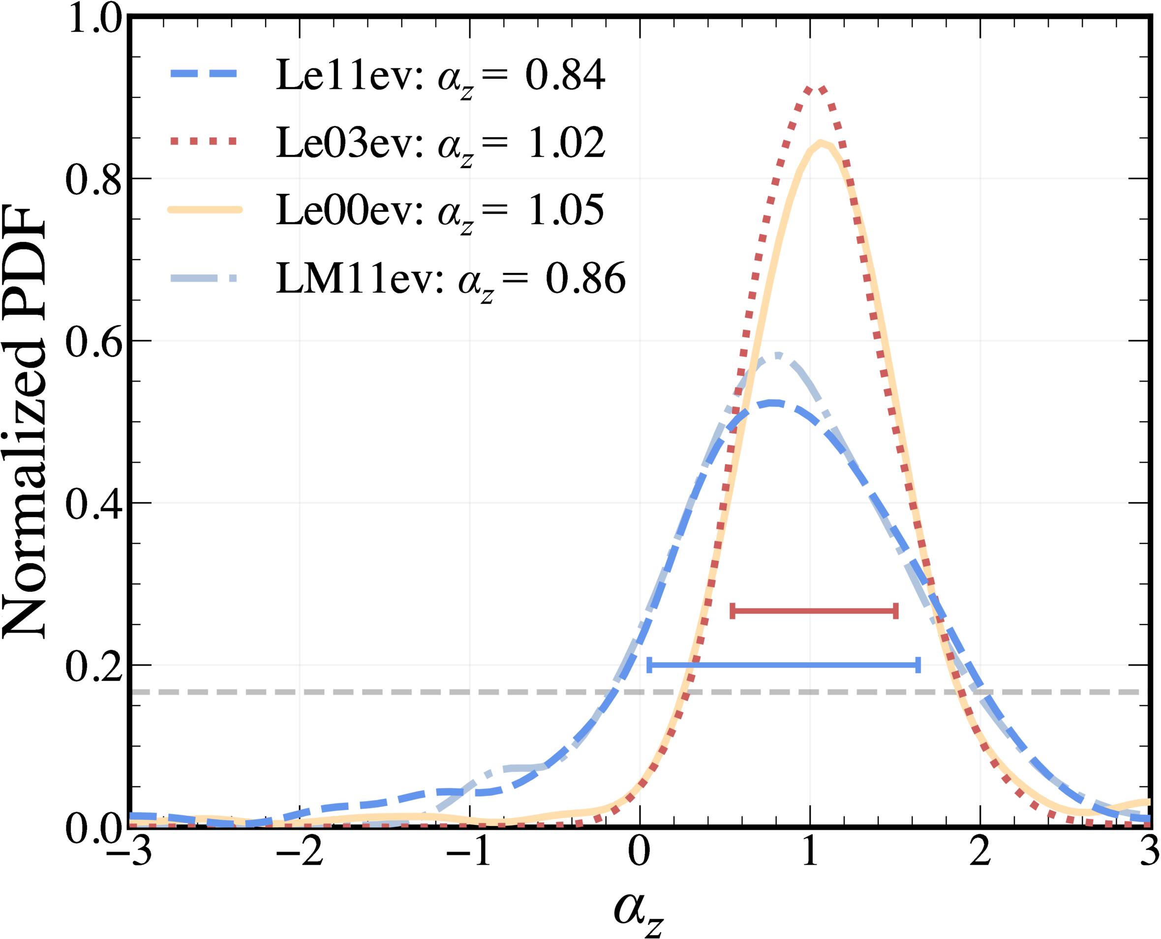
Figure 1. Refer to the following caption and surrounding text. — **Figure 1.** Here we show the four posterior distributions for α_z from our models. The upper red and lower blue horizontal lines indicate the 68% confidence region for Le03ev and Le11ev; the gray dashed line shows our uniform prior. These are functionally identical to those of LM11ev and Le00ev, respectively. In each distribution 87.2%–99.3% of values are positive, indicating a moderate to strong positive evolution in the M_BH–M_bulge amplitude. The posterior distributions for our models fall into two categories: (i) a wide range of α_z values with a significant (greater than 10%) fraction of the distribution falling below α_z = 0, and (ii) a very narrow, nearly symmetrical distribution of α_z values with only a negligible (under 5%) fraction of the distribution sitting below α_z = 0. This first category corresponds to models that sampled all 11 GSMF parameters (Le11ev and LM11ev); these distributions, while largely positive, are consistent with no significant redshift evolution of the M_BH–M_bulge relation. The latter category, however, shows strong evidence for a positive M_BH–M_bulge amplitude evolution. The distributions from this second category had some or all of the GSMF parameters fixed (Le03ev and Le00ev) in the prior setup. With fewer degrees of freedom these models converged to higher values of α_z to a higher degree of confidence, suggesting a better constraint for the M_BH–M_bulge amplitude evolution than the larger models. This is indicative of the degeneracy between the GSMF and M_BH–M_bulge parameters in our models.
Download figure:
Standard image High-resolution image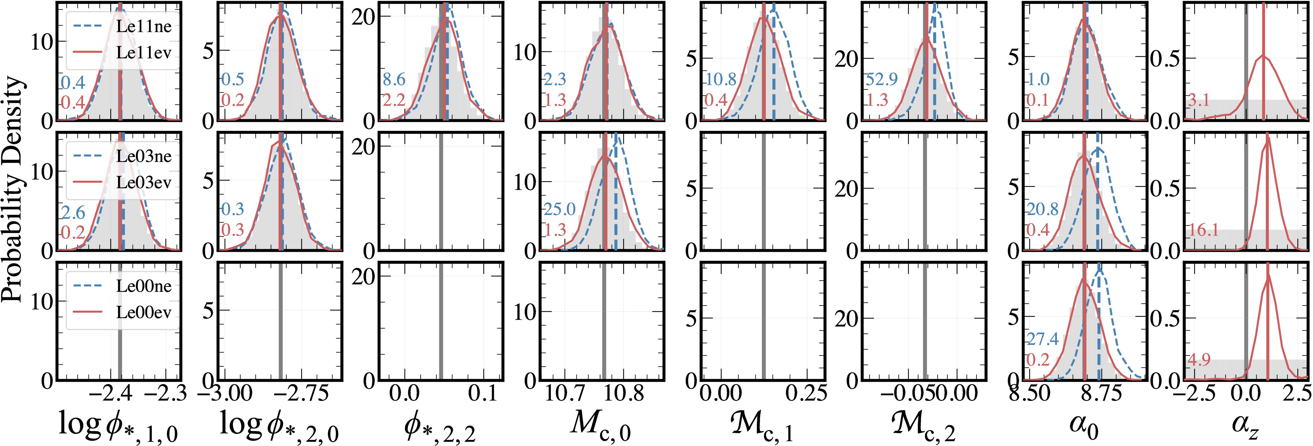

Figure 2. Refer to the following caption and surrounding text. — **Figure 2.** The posterior distributions for each of the evolving (red solid) and nonevolving (blue dashed) models. The priors are represented by the gray histograms in each panel, and the gray vertical lines indicate the fiducial values. Each row represents a different evolving/nonevolving M_BH–M_bulge model pair: Le11ne and Le11ev (top), Le03ne and Le03ev (middle), and Le00ne and Le00ev (bottom). In the case where a parameter was fixed, there is no histogram and only the vertical line is shown. In each panel we show the Kullback–Leibler divergence, D_KL, between each model posterior and the prior. The top, blue number is for the Le_ne models and the bottom, red number is for Le_ev models. For each parameter, D_KL is equal to or lower for models which allow for M_BH–M_bulge evolution, indicating that the posterior distributions are in equal or better agreement with the priors when compared to the fixed α_z = 0 counterparts. All three posterior distributions for α_z (rightmost column) demonstrate a preference for positive values. The α_z posterior is relatively broad for the top row (Le11ev), but when the evolutionary GSMF parameters are fixed (Le03ev, middle row) the distribution shifts toward higher values and also narrows. When only the local GSMF parameters were sampled but α_z was fixed to 0 (Le03ne), the posterior distributions deviated from the priors, not only for GSMF parameters (e.g., M_c,0, M_c,1, and M_c,2) but also for α₀. When α_z is allowed to vary, the posteriors recover the prior GSMF parameters. Additionally, when any number of the GSMF parameters are fixed (bottom two rows, Le03ev and Le00ev), the α_z = 0 models return high posterior values for the local M_BH–M_bulge amplitude, α₀. This is indicative of the degeneracy between increasing galaxy number density and increasing M_BH–M_bulge amplitude (either locally and/or at high z). We also see little change between α₀ and α_z posteriors in the middle and lower rows, suggesting that fixing the three local GSMF parameters (Le00ev) does not have a further effect over fixing only the evolutionary parameters. Overall, the models that allow the M_BH–M_bulge relation to evolve are otherwise in better agreement with observational constraints for the GSMF and local M_BH–M_bulge amplitude, and have posterior distributions for α_z that are between 87% and 99% positive.
Download figure:
Standard image High-resolution image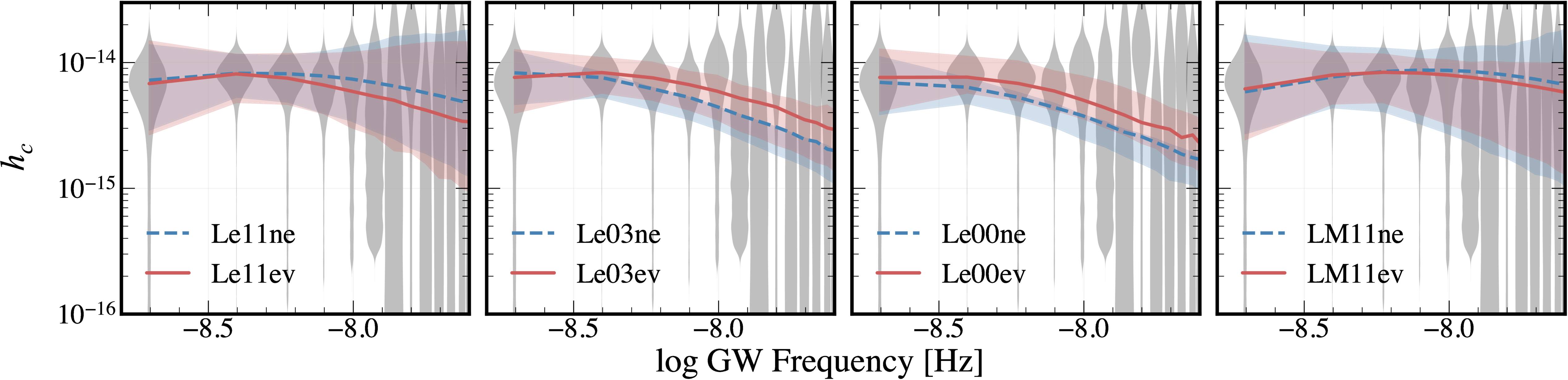

Figure 3. Refer to the following caption and surrounding text. — **Figure 3.** The GWB spectra associated with the best-fit parameters from our eight models fit to the first five frequency bins. The blue dashed lines indicate models with α_z fixed to zero, and the red solid lines indicate models which allowed for M_BH–M_bulge evolution. In all four panels, the spectra from the evolving M_BH–M_bulge models are in good agreement with the data, though we note that the likelihood value for Le00ev is the lowest of the eight models (discussed further in Section 3.4 and Appendix C). There are some differences between the slope of the high-frequency end, but this portion of the spectrum is poorly constrained and it is not possible to distinguish between goodness of fit in this regime at this time. When all GSMF parameters are sampled (left- and right-hand panels, Le11ne and LM11ne), the spectra are nearly identical between the evolving and nonevolving models. The models with some/all GSMF parameters fixed (Le03ne and Le00ne) show more significant differences between the evolving and nonevolving models. For these models, those which allowed α_z to vary are consistently in better agreement with the data than the fixed α_z = 0 counterparts, indicating that these evolving models are a better description of the GWB than their nonevolving counterparts.
Download figure:
Standard image High-resolution image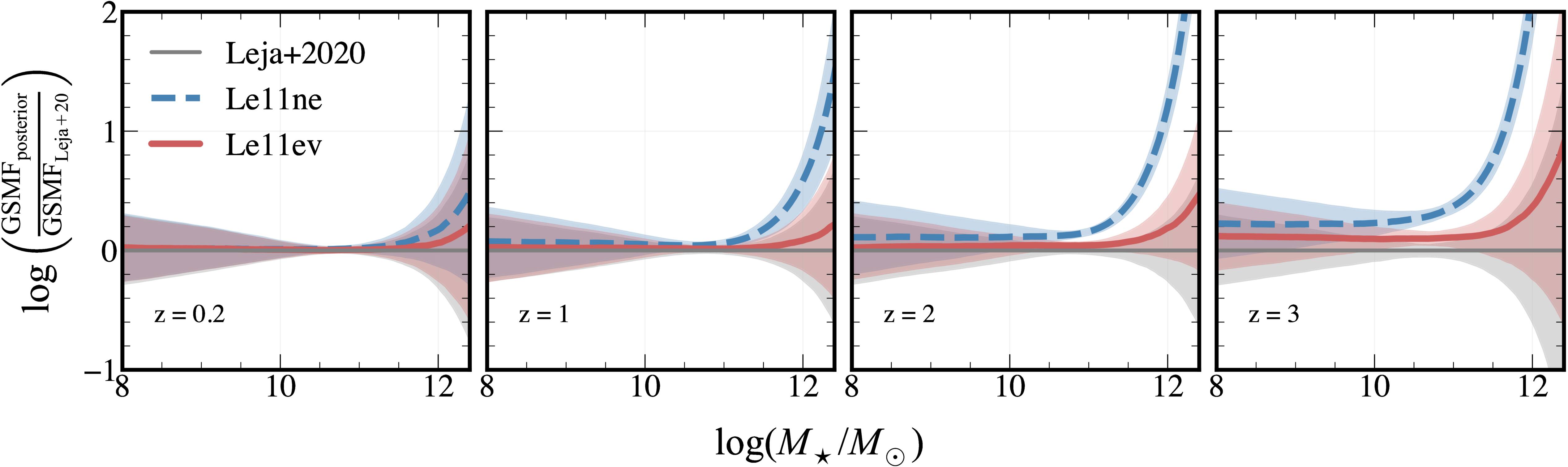

Figure 4. Refer to the following caption and surrounding text. — **Figure 4.** Here we plot the difference between the posterior GSMF from both the evolving (Le11ev, red solid) and nonevolving (Le11ne, blue dashed) M_BH–M_bulge models and the observed GSMF from J. Leja et al. (2020). The light gray region represents the 1σ error in the GSMF from J. Leja et al. (2020); we show the equivalent error range for Le11ne in blue and for Le11ev in red. We compare the models only within the redshift range used in J. Leja et al. (2020): 0.2 < z < 3. We see that, when the M_BH–M_bulge relation is not allowed to evolve, the GSMF shows a higher number density of high-mass galaxies with an increasing discrepancy as redshift increases. This difference is highest for galaxies with M_⋆ > 10¹¹M_⊙, though by z = 3 the posterior GSMF from Le11ne is inconsistent with the observed GSMF at all masses M_⋆ > 10⁹M_⊙. When the M_BH–M_bulge amplitude is allowed to evolve, however, the posterior GSMF is consistent within the uncertainties of the observed GSMF, though with a minor positive offset. This difference is evidence that our best-fit models with an evolving M_BH–M_bulge amplitude are in better agreement with observational constraints for galaxy number density than the nonevolving models.
Download figure:
Standard image High-resolution image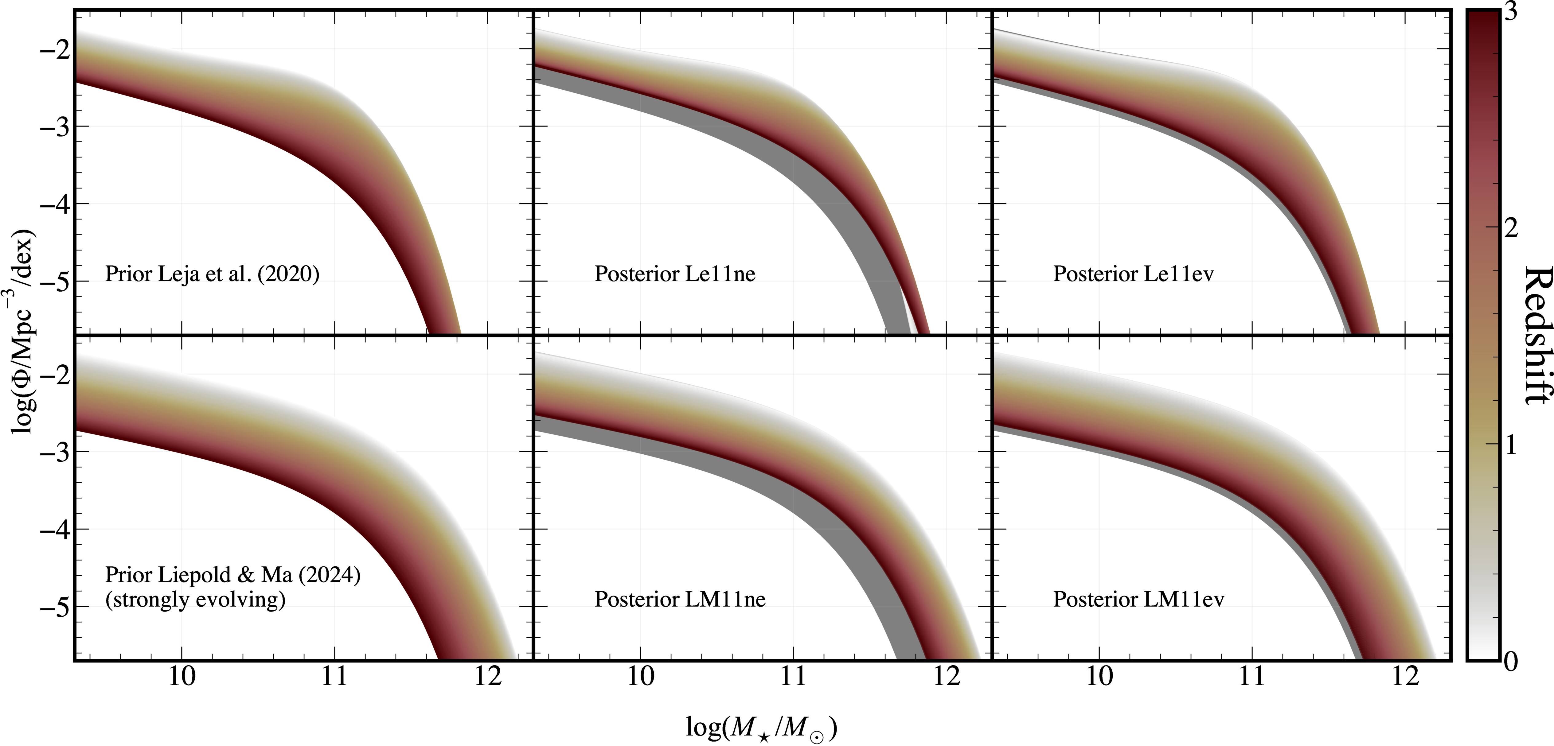

Figure 5. Refer to the following caption and surrounding text. — **Figure 5.** Top left: the prior GSMF from J. Leja et al. (2020). Top middle: the posterior GSMF for Le11ne. Top right: the posterior GSMF for Le11ev. Bottom: same as top row, but for models based on our strongly evolving version of the E. R. Liepold & C.-P. Ma (2024) GSMF. We see that, in both middle plots, the models which have α_z = 0 require a large number density of galaxies relative to their respective fiducial model. Despite the increased local number density, the posterior GSMF from LM11ne returns a greater number density for z = 3 compared to the J. Leja et al. (2020) GSMF. The prior for this model had a similar number density to that of J. Leja et al. (2020) in this redshift range, by design. The number densities for 2 ≲ z ≲ 3 are similar between the two posterior models with α_z = 0. This means that, to reproduce the GWB without an evolving M_BH–M_bulge amplitude, we need a significantly higher number density of massive galaxies out to z ∼ 3. For both models that allowed α_z to vary (rightmost panels), the posterior GSMFs are only negligibly different from the priors and the corresponding median posterior values for α_z are similar (see Figure 1 and Table 2), implying that the locally increased number density for LM11ev does not sufficiently increase the GWB amplitude without additionally increasing the high-z GSMF number density or the M_BH–M_bulge amplitude.
Download figure:
Standard image High-resolution image

In Section 3.4, we present our analysis of the GSMF parameters, which we then further discuss in Section 4.

3.1. Full-sample Models

Here we present the results of models that sampled all 29 (30 with α_z) parameters. First, we describe the outcome of the models that used our fiducial GSMF from J. Leja et al. (2020); we then present the impact of our test cases for explicitly evolving GSMF based on E. R. Liepold & C.-P. Ma (2024).

3.1.1. Le11ne and Le11ev

For the majority of parameters, the posterior distributions recover the priors for both Le11ne and Le11ev. In the top row of Figure 2, we highlight eight parameters from these models; we discuss the effects of the remaining parameters in Appendix C, and complete corner plots can be found in Appendix D. The nonevolving model, Le11ne, shows slight deviations toward higher values for three of the the GSMF characteristic mass and normalization evolutionary parameters (ϕ_*,2,2, M_c,1, and M_c,2). The two posterior distributions with the largest deviations from the priors are both of the evolutionary parameters for the characteristic stellar mass. When the M_BH–M_bulge relation is allowed to evolve, the posterior distributions for Le11ev are more consistent with the priors for all GSMF parameters, though there is still a mild offset in the same direction as Le11ne for ϕ_*,2,2. The posterior distribution for α_z is 87.2% positive, with a median value of 0.85. A Savage–Dickey ratio test in favor of the evolving model returns a value of 1.3, which indicates that this fit is consistent with no M_BH–M_bulge evolution.

The local GSMF values are recovered in both models, but the nonevolving model posteriors return generally larger values for the M_c evolutionary parameters. Higher values for M_c,1 and M_c,2 produce greater number densities of galaxies at higher redshifts, while maintaining consistency with the fiducial local number density. In particular, larger values for the characteristic mass produce more massive galaxies and therefore a greater number of massive SMBHs.

We use D_KL to quantify the deviation of the posteriors from the priors for Le11ne and Le11ev. Two distributions with D_KL = 0 are equivalent, whereas D_KL > 0 indicates disagreement. For all the parameters shown in Figure 2, the value of D_KL for Le11ne is equivalent or greater than for Le11ev. This means that the posterior distributions for Le11ne diverge from the priors more than in Le11ev, suggesting that the posterior distributions for Le11ev are in better agreement with the observed GSMF and local M_BH–M_bulge relation.

Figure 4 (see also Figure 5) compares the GSMF from J. Leja et al. (2020) to the GSMFs implied by the median posterior values from Le11ne and Le11ev. In the local Universe, all three GSMFs are in good agreement. By z = 2, both GSMFs from Le11ne and Le11ev lie above the observed values, though Le11ev is consistent, within error bars, with J. Leja et al. (2020). The difference between the GSMFs becomes larger with redshift, with Le11ev remaining consistent with the observed GSMF, while Le11ne is 0.5–2 orders of magnitude greater for galaxies with M_⋆ ≥ 10^10.5M_⊙ at z = 3. These massive galaxies host the SMBHs in the mass range that dominates the GWB signal (M_BH > 10⁹M_⊙; G. Agazie et al. 2023b). When predicting SMBH masses using the local M_BH–M_bulge relation, to increase the amplitude of the modeled GWB, we need an increased number density of these massive galaxies compared to the fiducial model. Alternatively, an evolving M_BH–M_bulge relation offers a way to increase the number density of the most massive SMBHs without changing the galaxy population or the locally observed SMBH–galaxy relation. This suggests that the best-fit parameters for models with an evolving M_BH–M_bulge amplitude are more consistent with observational constraints than nonevolving models.

3.1.2. LM11ne and LM11ev

We find an anticorrelation between the strength of the GSMF evolution we assume and the resulting GWB amplitude. A strongly evolving GSMF (larger values of M_c,i) predicts lower mass densities of galaxies relative to a weakly evolving GSMF (lower values of M_c,i). The strongly evolving GSMFs also therefore produce lower number densities of the most massive SMBHs, which then produces lower GWB amplitudes.

Despite the greatly increased number density of local galaxies in this model, the strongly evolving GSMF produces a GWB spectrum that is only marginally greater in amplitude than the fiducial model. In fact, the posterior distributions, using the strongly evolving E. R. Liepold & C.-P. Ma (2024) GSMF (with its much higher number density of galaxies with M_⋆ ≥ 10^11.5M_⊙), display similar behavior to those of Le11ne and Le11ev. That is, the GSMF posteriors for models without M_BH–M_bulge evolution tend toward greater number densities of high-mass galaxies for z ≳ 1. The GSMF posteriors recover the priors when M_BH–M_bulge evolution is allowed and the posterior distribution for α_z is nearly identical to that of Le11ev (see Figure 1).

In Figure 5, we compare the prior and posterior GSMFs for all full-sample models. We see that the galaxy number densities for 1 ≲ z < 3 are roughly equivalent for Le11ne and LM11ne (similarly for Le11ev and LM11ev). We see a more significant difference between models that have an evolving or static M_BH–M_bulge relation than between models with different prior GSMFs (further discussed in Section 3.4). This result suggests that, to reproduce the GWB amplitude, we need a significantly greater number density of galaxies than we currently observe, not only locally but at least out to z = 3. We discuss the physical implications and feasibility of this model further in Section 4.

While the local GSMF measured by E. R. Liepold & C.-P. Ma (2024) offers valuable insight into the local galaxy population and the limits of volume-limited surveys, we do not find that this local increase in galaxy number density is sufficient to reproduce the observed GWB spectrum. The difference between our result and what E. R. Liepold & C.-P. Ma (2024) find is a direct result of the assumptions made about binary hardening mechanisms in our respective calculations. For their estimate of the GWB amplitude, E. R. Liepold & C.-P. Ma (2024) follow the methods of G. Sato-Polito et al. (2024) and E. S. Phinney (2001). This model includes only the effect of gravitational-wave-driven SMBH binary hardening, which produces a power-law spectrum. In this work, we assume that binaries can also harden through dynamical friction and stellar scattering. The effect of these additional hardening pathways is to change the shape of the overall spectrum and to lower the amplitude. While keeping all other parameters constant, the change in shape and amplitude has the greatest impact at the low-frequency end of the spectrum (f ≲ 10 nHz; see, e.g., the lower-right panel of Figure 4 in G. Agazie et al. 2023a). The shape of the spectrum when including these additional hardening mechanisms provides better fits to the data across the observed range of frequencies than the gravitational-wave-only model (G. Agazie et al. 2023a).

3.2. Fixed GSMF Evolution Models: Le03ne and Le03ev

The first of the submodels that we discuss are Le03ne and Le03ev. Each of these is identical to Le11ne and Le11ev, respectively, except the six evolutionary parameters (ϕ_*,1,1, ϕ_*,1,2, ϕ_*,2,1, ϕ_*,2,2, M_c,1, and M_c,2) alongside α₁ and α₂ for the GSMF are fixed to the posterior values given by J. Leja et al. (2020). To focus on the degeneracy between the GSMF and M_BH–M_bulge parameters, we additionally fixed all parameters for galaxy merger rates and bulge fractions to their fiducial values. These models therefore sample a total of eight parameters (nine with α_z).

When sampling from all 11 GSMF parameters, the posteriors for the model that did not allow for M_BH–M_bulge evolution (Le11ev) recovered the priors for the local GSMF values, while only the evolutionary parameters deviated. Now, since these evolutionary parameters were fixed, the local GSMF posterior for characteristic mass is distributed toward greater values. Unlike before, this model also returns a posterior distribution with generally larger values of the M_BH–M_bulge amplitude than the prior. An increase to either the characteristic galaxy mass or the M_BH–M_bulge amplitude can generate the top-heavy BHMFs necessary to reproduce the observed GWB. A moderate (within 1σ) increase to both parameters, on the other hand, allows for massive SMBH populations to be modeled without deviating too far from either one parameter. This result is consistent with that found by G. Agazie et al. (2023b): To match the GWB, either a large number of parameters in the fiducial model must change by a small amount, or a very small number of parameters must differ significantly.

When the M_BH–M_bulge relation is allowed to evolve, the posterior distributions for all GSMF parameters are in good agreement with the priors. Interestingly, the distribution for α_z for this model is 99.3% positive with a Savage–Dickey ratio of 24.6. The standard deviation of this distribution is also significantly reduced, indicating a higher confidence of positive evolution.

Similar to Le11ne versus Le11ev, the D_KL between the priors and posteriors for Le03ne is equivalent or greater than for Le03ev. As mentioned earlier, the posterior distributions for M_c,0 and α₀ diverge from the priors more significantly in Le03ne than in Le11ne. In Le11ne the two distributions with the highest divergence were M_c,1, and M_c,2. These values are fixed in Le03ne, and so this model compensates by increasing M_c,0, and α₀. We do not see a notable change to the D_KL values for these distributions in Le00ev versus Le11ev.

Nearly all samples from the model that did not include M_BH–M_bulge evolution tend toward lower GWB amplitudes. In the second panel of Figure 3, we see that the shape of the GWB spectrum is nearly straight. Except for the two rightmost frequency bins, the best-fit spectrum is equivalent to the upper limit on the models, meaning that no models produced a GWB amplitude higher than the best-fit model for the higher frequencies. The best-fit model here is roughly consistent (though on the low side) with four of the five frequency bins we used for fitting. The Le03ev model, on the other hand, while lower in GWB amplitude than Le11ev at the high-frequency end, is still consistent with the PTA data.

3.3. Fixed GSMF Models: Le00ne and Le00ev

Finally, we present the smallest subset of our models, which only sample the three hardening parameters, the M_BH–M_bulge amplitude, and α_z (for Le00ev). These models fix all 11 GSMF parameters to their fiducial values from J. Leja et al. (2020), so the local and high-z GSMF cannot vary for these models.

This subset of models returns a posterior α_z distribution that is 96.8% positive with a Savage–Dickey ratio of 5.2. In this case, the posterior distribution for the M_BH–M_bulge amplitude recovers the prior almost exactly. For the nonevolving model, to reproduce high SMBH masses a greater overall M_BH–M_bulge amplitude is required. This result demonstrates how the models will trend more strongly toward positive values of α_z as the other options for increasing the number density of massive SMBHs are removed. When the option for evolution is also removed, the posteriors will deviate strongly from the priors for parameters that are influential on the predicted SMBH number density.

The GWB spectra share similar characteristics to the Le03ne and Le03ev models, with the non-M_BH–M_bulge evolving models consistently lying below the majority of the PTA data, and the evolving M_BH–M_bulge models falling closer to the center of the violins in more bins, but lying slightly above the median. We note that the best-fit spectrum for Le00ne has the lowest likelihood of all eight spectra, indicating it is the worst fit to the GWB, an effect we detail further in Appendix C.

3.4. Influence of the GSMF

In this section, we present the posterior GSMFs in two ways. We show the posterior GSMFs overplotted with the corresponding prior GSMFs for the full-sample models in Figure 5 for visual comparison. We then quantify the number density increase relative to J. Leja et al. (2020), which we plot versus the corresponding α(z) posterior median to demonstrate the degeneracy between these quantities in Figure 6.

Figure 6. Refer to the following caption and surrounding text. — **Figure 6.** The quantity Ξ represents the normalized number density “boost” in a given posterior GSMF relative to the corresponding fiducial GSMF for $11\lt {\mathrm{log}}{M}_{\star }\lt 13$ and 0.5 < z < 3. Ξ = 0 means the two GSMFs are equivalent, and a positive value of Ξ corresponds to an increased number density relative to the fiducial model across our integration range; all Ξ values were normalized to a maximum of 1. Red points are for models that allow the M_BH–M_bulge relation to evolve and blue points fixed α_z to be 0. The size of the points corresponds to the log-likelihood value of the best-fit GWB spectrum. Larger circles indicate better fits to the GWB data, while low values of Ξ indicate better agreement with the GSMF. Therefore, models which are consistent with both datasets have large marker sizes and are low on the y-axis. Each model pair shares a marker style overlaid in white (e.g., Le11ne and Le11ev are blue and red circles with stars). There is a clear negative correlation between pairs and also across all models. This demonstrates the degeneracy between an increased number density of galaxies and an increased SMBH–galaxy mass ratio. This degeneracy exists because both are valid pathways for producing the high number density of massive SMBHs implied by the GWB.
Download figure:
Standard image High-resolution image

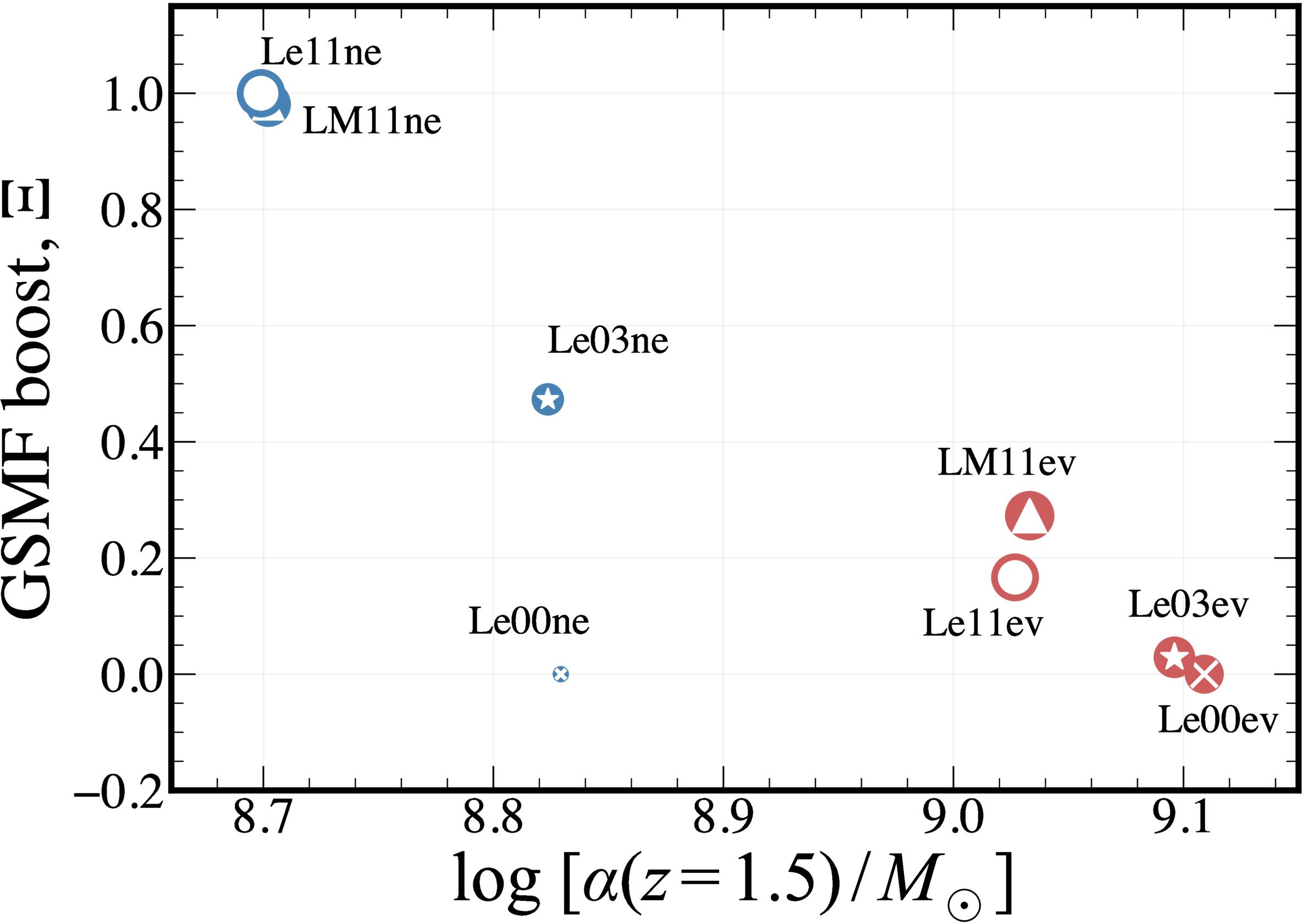
**Figure 6.** The quantity Ξ represents the normalized number density “boost” in a given posterior GSMF relative to the corresponding fiducial GSMF for $11\lt {\mathrm{log}}{M}_{\star }\lt 13$ and 0.5 < z < 3. Ξ = 0 means the two GSMFs are equivalent, and a positive value of Ξ corresponds to an increased number density relative to the fiducial model across our integration range; all Ξ values were normalized to a maximum of 1. Red points are for models that allow the M_BH–M_bulge relation to evolve and blue points fixed α_z to be 0. The size of the points corresponds to the log-likelihood value of the best-fit GWB spectrum. Larger circles indicate better fits to the GWB data, while low values of Ξ indicate better agreement with the GSMF. Therefore, models which are consistent with both datasets have large marker sizes and are low on the y-axis. Each model pair shares a marker style overlaid in white (e.g., Le11ne and Le11ev are blue and red circles with stars). There is a clear negative correlation between pairs and also across all models. This demonstrates the degeneracy between an increased number density of galaxies and an increased SMBH–galaxy mass ratio. This degeneracy exists because both are valid pathways for producing the high number density of massive SMBHs implied by the GWB.
Download figure:
Standard image High-resolution image

In Figure 5, we can see that the posterior GSMFs from Le11ne and LM11ne generally have higher number densities than the fiducial model. This offset is most extreme for the LM11ne GSMF, which is to be expected since the fiducial GSMF for this model started with a higher number density than the J. Leja et al. (2020) GSMF for z < 1. Both of these GSMFs are greater in number density than their respective fiducial model and the fixed α_z = 0 counterpart. Although we highlight the most extreme examples here, this trend is seen across models: Those with fixed α_z = 0 require a greater number density of galaxies, especially the most massive ones.

Because the GSMF is defined by up to 11 parameters in our models, the degeneracy between α(z) and any given GSMF parameter is not very strong. There is, however, considerable degeneracy between the M_BH–M_bulge evolution and an increased number density of galaxies. To further demonstrate this degeneracy, we define the quantity Ξ to be the integrated difference of the number density of galaxies between two models (see Equation (6)). We integrate over $11\lt {\mathrm{log}}{M}_{\star }\lt 13$ in mass and 0.5 ≤ z ≤ 3 in redshift, and note that the trend of the results from this analysis is not sensitive to the bounds of our integral. We chose to omit 0 < z < 0.5 in the integration range for clarity; including this range only results in a constant positive offset in Ξ for both LM11ne and LM11ev. We additionally normalize Ξ such that all our values lie between 0 and 1; Ξ = 0 indicates that the posterior GSMF is equivalent to the prior GSMF across our integration range (which is the case for both Le00ne and Le00ev). The Ξ parameter encapsulates the “boost” in galaxy number density and is analogous to the way α(z) encodes the changing M_BH–M_bulge amplitude:

In Figure 6, we plot Ξ against the M_BH–M_bulge amplitude at a fixed redshift α (z = 1.5). Locally all values of α(z) are equivalent, and the value of z we choose only shifts the evolving M_BH–M_bulge models left or right on the x-axis. The color differentiates evolving (red) models from nonevolving (blue), and the marker styles show the pairs of models with the same prior setup aside from M_BH–M_bulge evolution (i.e., each marker style appears twice, one on red and one on blue). The clear negative trend demonstrates the degeneracy between an increased number density of galaxies and an increased SMBH–galaxy mass ratio in our posterior models. In the cases where the GSMF was allowed to vary, the evolving models (Le11ev, Le03ev, Le00ev, and LM11ev) have a lower value for Ξ and a higher value for α(z = 1.5) than their nonevolving counterparts (Le11ne and Le03ne). These models follow the same trend, but are additionally boosted relative to the fiducial J. Leja et al. (2020) GSMF by design (as described in Section 2.3 and Appendix A). The only outlier to this trend is Le00ne. The best-fit likelihood value for this model is several orders of magnitude smaller than for other models (represented by the size of the points), indicating it is a poor fit to the GWB data. While in good agreement with the GSMF (low Ξ), its location on the plot is not an accurate reflection of the overall trend since the trend is defined by models that can reproduce the GWB. Therefore, we conclude that the high number density of massive SMBHs required to reproduce the GWB can be produced either by a large increase to galaxy number density (GSMF), a large increase to the SMBH–galaxy mass ratio, or a moderate increase to both.

The models that fix some/all GSMF parameters converge to higher values of α_z with a greater degree of confidence. The Le03ev model only fixed the evolutionary parameters from J. Leja et al. (2020) and sampled the local GSMF values. The posteriors for this model recovered the local GSMF and M_BH–M_bulge parameters, while its counterpart model, Le03ne, with α_z fixed to zero did not. This suggests that the GWB free spectrum is well described by a SMBH population, as predicted from an evolving M_BH–M_bulge relation and the galaxy number density given by the GSMF from J. Leja et al. (2020). The GWB spectrum is equally well described by an unchanging M_BH–M_bulge relation if—and only if—the GSMF is significantly higher in number density (for M_⋆ > 10^11.5M_⊙), not only locally but also out to z as high as 3, which is not well supported by observational data (e.g., A. Muzzin et al. 2013; A. R. Tomczak et al. 2014; I. Davidzon et al. 2017; P. Behroozi et al. 2020), though it is not entirely ruled out (e.g., J. Moustakas et al. 2013; A. H. Wright et al. 2018).

3.5. Black Hole Number Density

In Figure 7, we present the BHMFs resulting from our models for 0.25 ≤ z ≤ 2. We additionally plot the posterior single SMBH functions from Figure 13 in G. Agazie et al. (2023b) and our fiducial BHMF for comparison. The BHMFs for evolving models using the J. Leja et al. (2020) GSMF (Le11ev, Le03ev, and Le00ev) are nearly identical to each other, and so we plot one BHMF that is the median of all three models. We compare this to the posterior BHMF from LM11ev, and find that the BHMFs are broadly consistent for z > 0.5 but that of LM11ev is greater in number density for the most massive SMBHs for z < 0.5. This is to be expected since this is the same behavior seen in the respective GSMFs.

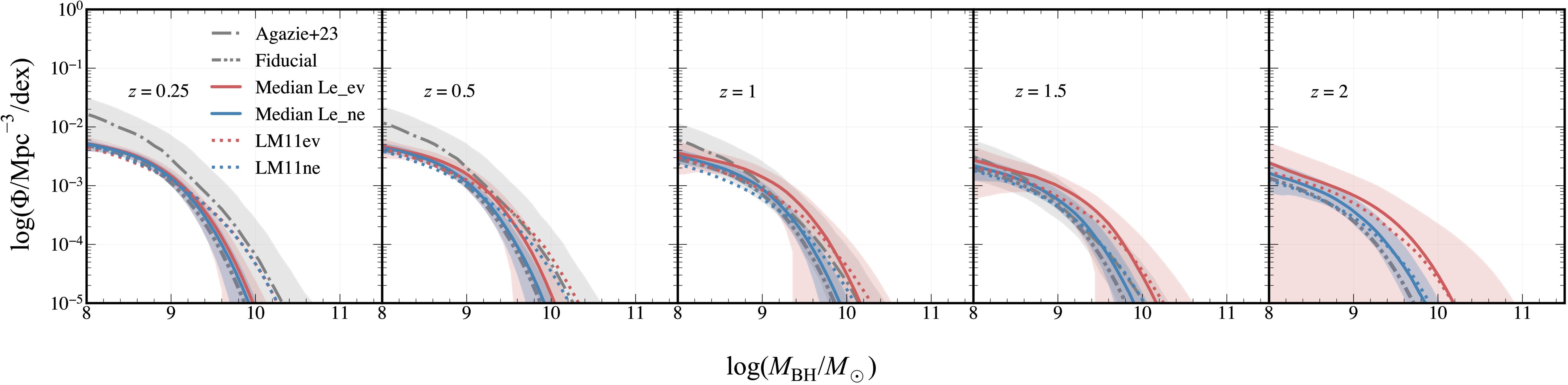
Figure 7. Refer to the following caption and surrounding text. — **Figure 7.** Posterior BHMFs from our best-fit models compared with the fiducial model and the BHMF from G. Agazie et al. (2023b). The red (blue) solid lines represent the median BHMF from all the evolving (nonevolving) models which used the J. Leja et al. (2020) GSMF. Models using the E. R. Liepold & C.-P. Ma (2024) follow this same color convention and are dotted instead of solid. We exclude Le00ne from these calculations because of its low likelihood value. Generally, the models that have an evolving M_BH–M_bulge have higher number densities at higher redshifts compared to the nonevolving counterparts. The models which used the J. Leja et al. (2020) GSMF and did not allow for M_BH–M_bulge evolution are mildly positively offset from the fiducial BHMF. This offset increases with redshift, reflecting the difference in posterior GSMF evolution.
Download figure:
Standard image High-resolution image

We also show the median BHMF for the fixed α_z = 0 models, Le11ne and Le03ne (excluding Le00ne due to its low likelihood). This BHMF has a lower number density than those of the evolving models across the entire mass range for z > 1. This BHMF is more similar to the fiducial BHMF for low redshifts, but has a boosted number density that increases with redshift. This increasing positive offset is reflective of the GSMF posteriors and the increased number density of galaxies in the nonevolving best-fit models (for Le11ne and Le03ne).

Generally, all posterior models have a higher number density of SMBHs relative to the fiducial model across all redshift bins, while evolving models typically have the highest number densities in a given bin.

Our results suggest that either the z = 0 M_BH–M_bulge relation does not apply at higher redshift or that galaxy observational surveys drastically underestimate the number of massive galaxies at all redshifts z < 3, either through nondetection of a population or by underestimating masses. The best-fit evolving models indicate a positive offset for the M_BH–M_bulge amplitude in the past. An M_BH–M_bulge amplitude that increases with redshift (α_z > 0) implies a black-hole-first evolution. Some studies have proposed this as a possible formation route, stating that kinetic-mode feedback from SMBH accretion disks can impede the star formation within the host galaxy, thus leading to a delayed stellar mass increase (M.-Y. Zhuang & L. C. Ho 2023), also known as black hole “dominance” (M. Volonteri 2012). In the opposite case, decreasing amplitude at high z may be indicative of radiative-mode feedback, where UV radiation from star formation prevents gas from sinking to the center of the galaxy, therefore postponing SMBH accretion (M.-Y. Zhuang & L. C. Ho 2023). Our results support the black hole dominance model of SMBH–galaxy coevolution. The value for the M_BH–M_bulge amplitude evolution we find, α_z = 1.04 ± 0.5, is consistent with several observational (X. Ding et al. 2020; F. Pacucci et al. 2023; Y. Zhang et al. 2023; T. S. Tanaka et al. 2025) and some theoretical/simulation (e.g., J. S. B. Wyithe & A. Loeb 2003; A. Cattaneo et al. 2005; D. J. Croton 2006) studies; however, there is a lack of consensus among these studies, especially for the redshifts most relevant for the GWB (e.g., A. Merloni et al. 2010; V. N. Bennert et al. 2011; M. Cisternas et al. 2011; J. Li et al. 2021). Our analysis places the strongest constraints only on the most massive SMBHs (M_BH ≥ 10⁸M_⊙). We cannot firmly differentiate between our power-law evolution and more complex models (such as dual-sequence behavior; T. Shimizu et al. 2024), nor can we determine whether the evolution is mass dependent (e.g., A. Hoshi et al. 2024). A complementary follow-up analysis could consider the effect of heavy versus light SMBH seeding models on the low-mass end of the M_BH–M_bulge relation to form a bigger picture of M_BH–M_bulge evolution.

In Figure 8, we show the M_BH–M_bulge amplitude offset ( ${\rm{\Delta }}{\mathrm{log}}{M}_{{\rm{BH}}}/{M}_{\odot }$ ) versus redshift predicted by our model alongside measurements from the literature. The gray scattered points represent individual galaxies with both stellar and SMBH mass measurements, and so we calculate the offset from the local M_BH–M_bulge relation for these objects. The lines represent models from papers that provide an explicit functional form or offset for M_BH–M_bulge evolution. The thicker red line and shaded red region represent the median posterior value for α_z and the 68% confidence region from our models with statistically significant evolution (Le03ev and Le00ev). We find that our model is most consistent with that from Y. Zhang et al. (2023, yellow dotted line), though our error bars encompass the models of J. S. B. Wyithe & A. Loeb (2003) and A. Merloni et al. (2010). We note that both A. Merloni et al. (2010) and M.-Y. Zhuang & L. C. Ho (2023) were careful to account for observational bias (e.g., as described by T. R. Lauer et al. 2007) in their analysis. Our model does not predict as extreme an offset as measured by X. Ding et al. (2020), F. Pacucci & A. Loeb (2024), or M. Yue et al. (2024).

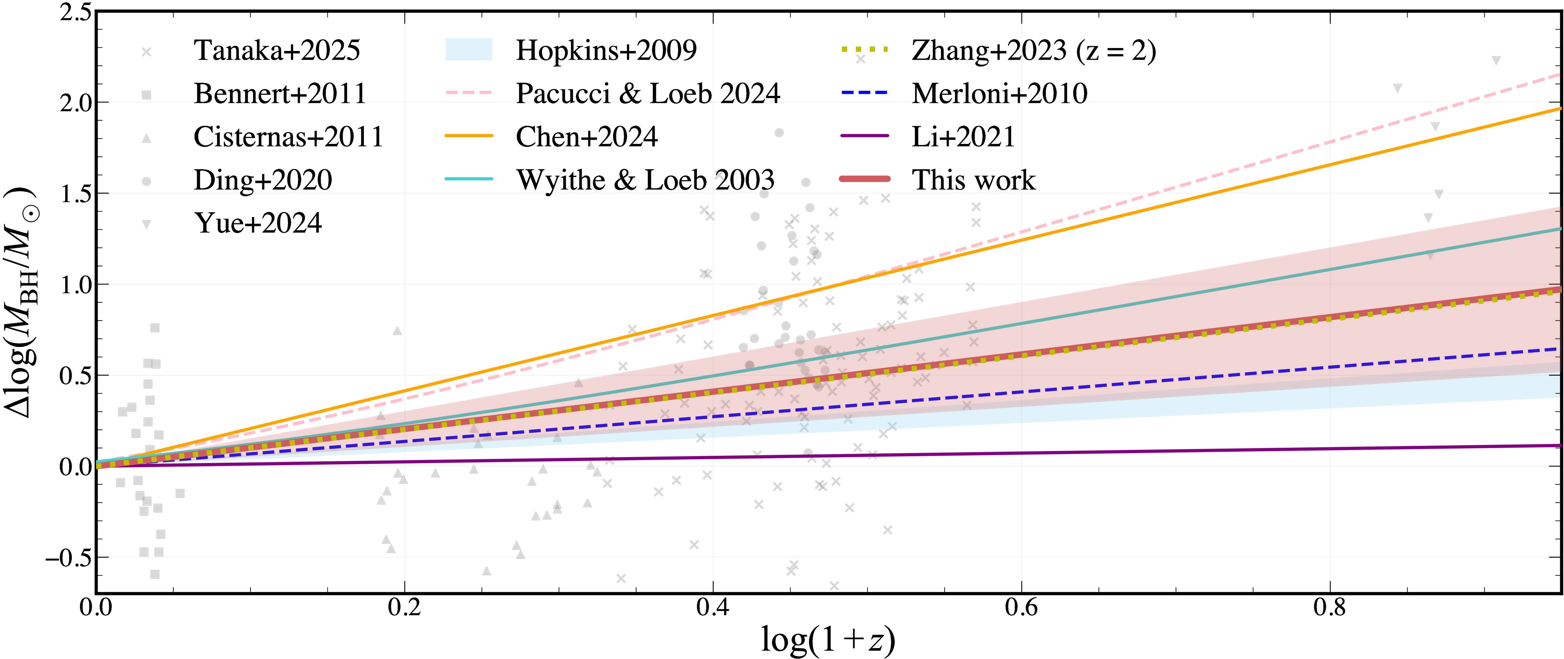
Figure 8. Refer to the following caption and surrounding text. — **Figure 8.** A comparison between different literature estimates of the M_BH–M_bulge relation and our results (thick, solid red line and 68% confidence shaded region). The y-axis is the (log) offset between SMBH mass at a given redshift compared to the local amplitude. For this figure, we include only our models with statistically significant evolution (Le03ev and Le00ev). The gray points represent data, while the different lines are the fitting results. For Y. Zhang et al. (2023, yellow dotted), we approximate the evolutionary form based on their reported redshift range and M_BH–M_bulge offset. Our analysis favors an intermediate positive evolution, which is nearly identical to that of Y. Zhang et al. (2023) and similar to those of J. S. B. Wyithe & A. Loeb (2003) and A. Merloni et al. (2010). Our model does not predict offsets as great as F. Pacucci & A. Loeb (2024), M. Yue et al. (2024), or Y. Chen et al. (2024).
Download figure:
Standard image High-resolution image

We find α_z = 1.04 ± 0.5, which lies below the value (α_z ∼ 2.07 ± 0.47) found by Y. Chen et al. (2024). Y. Chen et al. (2024) perform a similar analysis to the one we present here in which they fit the same data and also use the same fiducial M_BH–M_bulge relation as us. There are two key differences between their model and ours: (i) the GSMF, and (ii) the SMBH binary hardening model. They use the GSMF from P. Behroozi et al. (2020), which has notably different (both higher and lower) number densities to our fiducial model across the mass and redshift ranges we consider. Because the GSMF they assume is not uniformly offset from ours, the effect on their α_z estimate is not obvious, but this difference is certainly a contributing factor to this discrepancy. Another difference between our models is the hardening prescription for the SMBH binaries. The model they use is a more complex model than we used here (Y. Chen et al. 2020). Differences in binary hardening efficiency can affect the GWB amplitude. We are able to model the GWB using α_z ∼ 2.07 if we assume a hardening timescale that is much longer than currently supported values (by up to a factor of 10 times higher than reported in G. Agazie et al. 2023b). For this work, we assume a constant hardening timescale, and the discrepancy between these results is demonstrative of the need for realistic binary hardening models. Future testing with EM studies will be important for placing bounds on hardening timescales. Inferences for SMBH populations from the GWB are sensitive to the underlying models used for galaxy populations. The difference in our results demonstrates the importance of having robust and well-constrained models.

Our analysis here suggests that, if we can reproduce the high GWB amplitude through only changes to the GSMF, then this would require a significantly higher number density of the highest-mass galaxies at higher redshifts (at least out to z = 3). As they discuss in their paper, the increased number density that E. R. Liepold & C.-P. Ma (2024) find indicates that galaxy surveys are missing out on the population of the most massive galaxies (M_⋆ ≥ 10^11.5M_⊙) and/or the mass-to-light ratios underestimate galaxy mass for this population. Local surveys may miss out on this population of galaxies because the survey area is simply not large enough to include this otherwise rare population. For higher redshifts, however, the survey volume is sufficient to ensure completeness, and so the COSMOS (C. Laigle et al. 2016) and 3D-HST+CANDELS (R. E. Skelton et al. 2014) surveys used in J. Leja et al. (2020), for example, should be representative of the underlying population. This, combined with the abundance of reliable data, would suggest that the posterior GSMF at z > 1 required by our models to match the GWB spectrum is inconsistent with the true galaxy population. If however the initial mass function is bottom-heavy, like that assumed by E. R. Liepold & C.-P. Ma (2024), and minimally evolving (and therefore bottom-heavy at higher redshifts), then a GSMF like that in the bottom-middle panel of Figure 5 could be feasible. In either case, analyses of the GWB are most directly a probe of SMBH properties, so any inferences we draw about the GSMF are several steps removed and are therefore only implicit. Although it is still useful to discuss the degeneracies with the GSMF in our models, the GSMF estimates from this study should be treated with caution.

Gravitational-wave-based studies such as this offer a new probe of SMBH–galaxy mass scaling relations that can complement observational studies. Broadly speaking, there are two ways to observationally infer the SMBH mass function over cosmic time using only EM data: (i) black hole mass scaling relations combined with observations of galaxies, and (ii) models of Eddington ratio distributions combined with observations of AGN luminosity functions. These two methods have inferred incompatible SMBH mass functions, with galaxy-observation methods predicting higher densities than AGN-observation methods. A series of works (F. Shankar et al. 2016, 2019; E. Barausse et al. 2017) proposed a potential solution whereby the (nonevolving) mass scaling relations had much lower amplitude (possibly a result of unsubstantiated measurement biases) to lower the galaxy-observation results to be in line with the AGN-observation results. Our work here shows that the GWB spectrum is generally in line with the galaxy-observation results. Not only are the measured scaling relations not too low at z = 0, they are, if anything, higher amplitude at higher redshift, something which has also been noted by other studies (e.g., E. R. Liepold & C.-P. Ma 2024; G. Sato-Polito et al. 2024). One as yet underexplored possibility to reconcile these two observational results is that radiative efficiencies are lower by a factor of 2–5 than typically assumed for the brightest AGNs. This is outside the scope of this paper, but will be investigated in future studies.

Our analysis of the M_BH–M_bulge relation focused on evolution of the amplitude, however it is possible that the relation may be evolving in other ways. Recent work has suggested that a variety of growth pathways are likely to be relevant within galaxy populations and that they are encoded in the intrinsic scatter (M.-Y. Zhuang & L. C. Ho 2023; B. A. Terrazas et al. 2025; J. H. Cohn et al. 2025; H. Hu et al. 2025), where the local M_BH–M_bulge relation acts as a sort of “attractor” for SMBH–galaxy pairs as they evolve. This concept is not new (e.g., C. Y. Peng 2007; M. Hirschmann et al. 2010; A. Merloni et al. 2010; K. Jahnke & A. V. Macciò 2011), but has seen a lot of new analysis, especially in the last two years. In particular, M.-Y. Zhuang & L. C. Ho (2023) conducted a study of z ≤ 0.35 AGNs, and found that the scatter in the M_BH–M_bulge relation is greater in the early Universe, a finding substantiated recently by both gravitational-wave and simulation analyses (e.g., E. C. Gardiner et al. 2024; B. A. Terrazas et al. 2025). Furthermore, J. Li et al. (2025) measured the SMBH–galaxy mass ratios for AGNs at z ∼ 3–5, and found that they are consistent with the local population. Results such as theirs could be indicative of an increased scatter in the M_BH–M_bulge relation outside the local Universe. Biased observations of a high-scatter M_BH–M_bulge relation could appear artificially as an inflated amplitude. Future GWB studies similar to this will provide valuable insights into alternative evolutionary forms of the M_BH–M_bulge relation.

It is also possible that a scaling relation not based on galaxy mass may more accurately reproduce the highest-mass SMBH number density. It has been shown that the M_BH–M_bulge and M_BH–σ relations predict different BHMFs outside the local Universe (C. Matt et al. 2023) and that this has an impact on the predicted GWB amplitude (J. Simon 2023). On the other hand, N. J. McConnell & C.-P. Ma (2013) found that both the M_BH–M_bulge and M_BH–σ relations “saturate” toward the highest masses, underpredicting SMBH masses for the largest bright cluster galaxies. Further, an analysis by G. Sato-Polito et al. (2024) found that neither of the local relations can reproduce the high GWB amplitude. In either case, there is strong evidence to suggest that the local M_BH–M_bulge relation was different in the past in some way, and multimessenger studies such as this are an exiting route toward characterizing SMBH–galaxy coevolution.

In this work, we implemented an evolving M_BH–M_bulge model that improves our ability to reproduce the GWB while maintaining consistency with astrophysically constrained models. We adapted the holodeck semi-analytic model to test for evolution in the M_BH–M_bulge relation and fit models to the GWB free-spectrum from G. Agazie et al. (2023a). Our results show mild to strong preference for a positive evolution in the M_BH–M_bulge amplitude. When modeling the M_BH–M_bulge relation as ${M}_{\mathrm{BH}}={\alpha }_{0}{(1+z)}^{{\alpha }_{z}}{({M}_{\mathrm{bulge}}/1{0}^{11}{M}_{\odot })}^{{\beta }_{0}}$ , we find that α_z = 1.04 ± 0.5.

We also studied the degeneracy between the GSMF and M_BH–M_bulge relation. The GWB requires massive SMBHs, and we find that this population can be modeled with a top-heavy GSMF (which becomes a top-heavy BHMF via the local M_BH–M_bulge relation) or an increased M_BH–M_bulge amplitude (either via positive redshift evolution or a high local value). The M_BH–M_bulge relation remains the most influential component in GWB amplitude calculations. While an alternative GSMF offers an interesting solution, the GSMF has more robust observational constraints than the M_BH–M_bulge relation outside the local Universe. Moreover, the GWB is primarily a probe of SMBH properties, so any inference about the GSMF is a secondary calculation. We therefore conclude that a SMBH-first growth model provides the best fits to the GWB while maintaining a high degree of consistency with EM-based observational constraints.

Future work will investigate the effects of an evolving intrinsic scatter in the M_BH–M_bulge relation. It will also be important to test different evolutionary models using upcoming PTA data releases, which will have higher signal-to-noise ratios, to better differentiate between models.

The authors would like to thank Joel Leja and CJ Harris for insightful discussions, which aided and improved the interpretation of this work. The authors additionally thank the anonymous referee for their thoughtful comments, which led to an increase in the clarity of communication and analysis of our results.

L.B. acknowledges support from the National Science Foundation under award AST-2307171 and from the National Aeronautics and Space Administration under award 80NSSC22K0808. P.R.B. is supported by the Science and Technology Facilities Council, grant No. ST/W000946/1. S.B. gratefully acknowledges the support of a Sloan Fellowship, and the support of NSF under award No. 1815664. The work of R.B., R.C., X.S., J.T., and D.W. is partly supported by the George and Hannah Bolinger Memorial Fund in the College of Science at Oregon State University. M.C., P.P., and S.R.T. acknowledge support from NSF AST-2007993. M.C. was supported by the Vanderbilt Initiative in Data Intensive Astrophysics (VIDA) Fellowship. Support for this work was provided by the NSF through the Grote Reber Fellowship Program administered by Associated Universities, Inc./National Radio Astronomy Observatory. Pulsar research at UBC is supported by an NSERC Discovery Grant and by CIFAR. K.C. is supported by a UBC Four Year Fellowship (6456). M.E.D. acknowledges support from the Naval Research Laboratory by NASA under contract S-15633Y. T.D. and M.T.L. received support by an NSF Astronomy and Astrophysics grant (AAG) award No. 2009468 during this work. E.C.F. is supported by NASA under award No. 80GSFC24M0006. G.E.F., S.C.S., and S.J.V. are supported by NSF award PHY-2011772. K.A.G. and S.R.T. acknowledge support from an NSF CAREER award No. 2146016. A.D.J. and M.V. acknowledge support from the Caltech and Jet Propulsion Laboratory President’s and Director’s Research and Development Fund. A.D.J. acknowledges support from the Sloan Foundation. N.La. acknowledges the support from Larry W. Martin and Joyce B. O’Neill Endowed Fellowship in the College of Science at Oregon State University. Part of this research was carried out at the Jet Propulsion Laboratory, California Institute of Technology, under a contract with the National Aeronautics and Space Administration (grant No. 80NM0018D0004). D.R.L. and M.A.M. are supported by NSF grant No. 1458952. M.A.M. is supported by NSF grant No. 2009425. C.M.F.M. was supported in part by the National Science Foundation under grants No. NSF PHY-1748958 and AST-2106552. A.Mi. is supported by the Deutsche Forschungsgemeinschaft under Germany’s Excellence Strategy – EXC 2121 Quantum Universe – 390833306. The Dunlap Institute is funded by an endowment established by the David Dunlap family and the University of Toronto. K.D.O. was supported in part by NSF grant No. 2207267. T.T.P. acknowledges support from the Extragalactic Astrophysics Research Group at Eötvös Loránd University, funded by the Eötvös Loránd Research Network (ELKH), which was used during the development of this research. H.A.R. is supported by NSF Partnerships for Research and Education in Physics (PREP) award No. 2216793. S.M.R. and I.H.S. are CIFAR Fellows. Portions of this work performed at NRL were supported by ONR 6.1 basic research funding. J.D.R. also acknowledges support from start-up funds from Texas Tech University. J.S. is supported by an NSF Astronomy and Astrophysics Postdoctoral Fellowship under award AST-2202388, and acknowledges previous support by the NSF under award 1847938. O.Y. is supported by the National Science Foundation Graduate Research Fellowship under grant No. DGE-2139292. Anishinaabeg gaa bi dinokiiwaad temigad manda Michigan Kichi Kinoomaagegamig. Mdaaswi nshwaaswaak shi mdaaswi shi niizhawaaswi gii-sababoonagak, Ojibweg, Odawaag, minwaa Bodwe’aadamiig wiiba gii-miigwenaa’aa maamoonjiniibina Kichi Kinoomaagegamigoong wi pii-gaa aanjibiigaadeg Kichi-Naakonigewinning, debendang manda aki, mampii Niisaajiwan, gewiinwaa niijaansiwaan ji kinoomaagaazinid. Daapanaming ninda kidwinan, megwaa minwaa gaa bi aankoosejig zhinda akiing minwaa gii-miigwewaad Kichi-Kinoomaagegamigoong aanji-daapinanigaade minwaa mshkowenjigaade.

The University of Michigan is located on the traditional territory of the Anishinaabe people. In 1817, the Ojibwe, Odawa, and Bodewadami Nations made the largest single land transfer to the University of Michigan. This was offered ceremonially as a gift through the Treaty at the Foot of the Rapids so that their children could be educated. Through these words of acknowledgment, their contemporary and ancestral ties to the land and their contributions to the University are renewed and reaffirmed.

C.M. was the primary lead for the formal analysis and investigation of this project. C.M. led the writing and editing of this manuscript and produced all figures and models. C.M. and K.G. were responsible for the conceptualization and supervision of this work. C.M. and L.Z.K. developed and adapted the software and methodology applied here. K.G., L.Z.K., J.S., and L.B. provided useful feedback and comments as well as aided in scientific interpretation of the results. Additional NANOGrav members are listed in alphabetical order; each contributed toward the collaboration-wide endeavor of pulsar timing which culminated in evidence for the GWB. The work presented in this paper benefits from data collected and analyzed in the course of this search and would not be possible without this large-scale coordination.

Software: Astropy (Astropy Collaboration et al. 2013, 2018, 2022), SciPy (P. Virtanen et al. 2020), NumPy (C. R. Harris et al. 2020), Matplotlib (J. D. Hunter 2007), kalepy (L. Z. Kelley 2021), holodeck (G. Agazie et al. 2023b), ceffyl (W. G. Lamb et al. 2023).

In this section, we describe the form of evolution we assume for the GSMF used in LM11ne and LM11ev. We additionally explore the effects of alternative GSMFs not presented in the main text, and briefly investigate the implications for the GWB and high-z galaxy population. The different GSMFs and corresponding GWB spectra are shown in Figure 9 and the parameters for each GSMF are shown in Table 3. We also describe the effect of the M_BH–M_bulge version on the predicted GWB spectrum at the end of this section and in Figure 10.

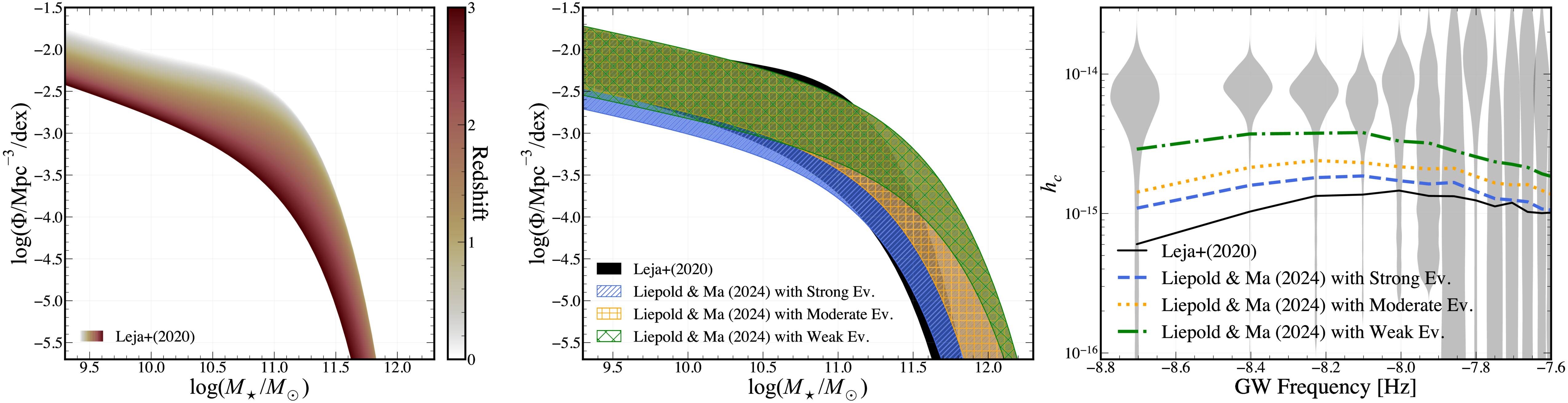
Figure 9. Refer to the following caption and surrounding text. — **Figure 9.** A comparison between the J. Leja et al. (2020) GSMF (left red/blue and middle black) and our evolving versions of the E. R. Liepold & C.-P. Ma (2024) GSMF (middle blue, orange, and green). The right panel shows the corresponding fiducial GWB spectra corresponding to each of these models. The GSMFs in the right and middle panels are all defined for 0 < z < 3. The strongly evolving GSMF (blue) we consider differs only negligibly from that in J. Leja et al. (2020) for M_⋆ ≥ 10¹¹M_⊙ (which corresponds to the SMBH masses contributing to the GWB the most) for z ≥ 1. In this case, we only see a minimal increase in amplitude to the GWB spectrum. In fact, even the weakly evolving GSMF (green) falls just short of the GWB data, indicating that a nearly nonevolving GSMF would be needed to match the GWB without changing other model parameters. For all GWB spectra shown here, we use the J. Kormendy & L. C. Ho (2013) M_BH–M_bulge relation.
Download figure:
Standard image High-resolution image

The GSMF measured by E. R. Liepold & C.-P. Ma (2024) uses only z = 0 galaxies, and so the authors do not provide an explicit evolutionary form for the GSMF at higher redshift. For use in our analysis, we construct and test several models that bracket the plausible rates of GSMF evolution. A strongly evolving GSMF is predicted for 0 < z < 1 (e.g., G. De Lucia et al. 2007), though observations often show a lack of evolution in this redshift range (e.g., J. Moustakas et al. 2013; K. Bundy et al. 2017; J. Leja et al. 2020). The E. R. Liepold & C.-P. Ma (2024) GSMF offers observational support for this predicted evolution. The GSMF from J. Leja et al. (2020) does not show significant evolution for 0 < z < 1, which, according to E. R. Liepold & C.-P. Ma (2024), could be due to observational biases in the local Universe. Large cosmological surveys do not have the appropriate local volume to catch the most massive galaxies, and so the E. R. Liepold & C.-P. Ma (2024) GSMF offers to complete the picture for the local high-mass GSMF. The J. Leja et al. (2020) GSMF is consistent with many other studies and theory for 1 < z < 3, and there is no strong foundation to believe that the GSMF in this redshift range is invalid. We can assume that the J. Leja et al. (2020) GSMF is complete for z ≳ 1 and therefore find an approximate evolution that matches the local E. R. Liepold & C.-P. Ma (2024) GSMF as well as the J. Leja et al. (2020) for z ≳ 1.

Starting with the explicit z = 0 GSMF from E. R. Liepold & C.-P. Ma (2024) and assuming a similar functional form to that in J. Leja et al. (2020), we tested three different forms of evolution represented by the shaded regions in Figure 9: (i) weakly evolving (green), producing a GWB amplitude similar to that in E. R. Liepold & C.-P. Ma (2024), (ii) moderately evolving (orange), and (iii) strongly evolving (blue), designed to match the high-mass end of the J. Leja et al. (2020) GSMF by a redshift of z ≳ 1. The model parameters are given in Table 3.

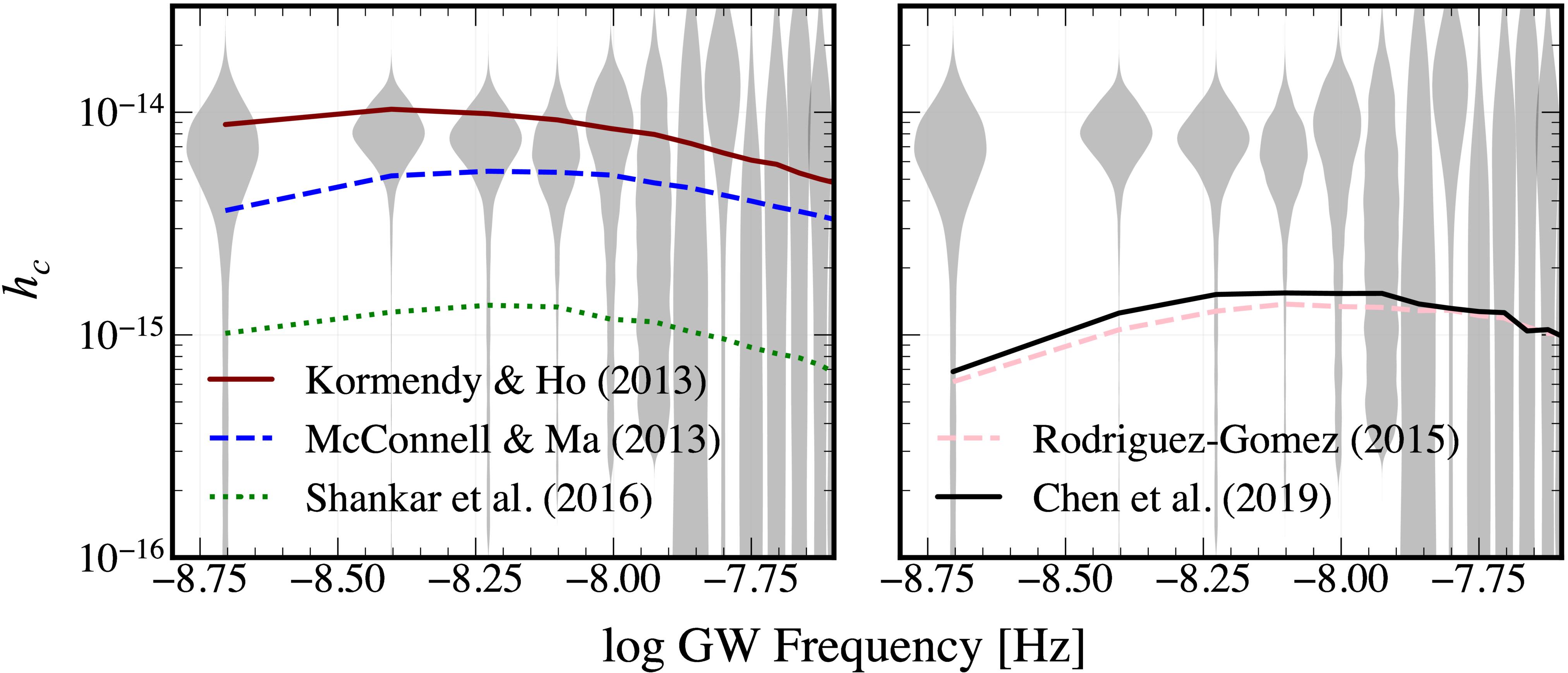
Figure 10. Refer to the following caption and surrounding text. — **Figure 10.** Left: panel demonstrating how the choice in scaling relation between J. Kormendy & L. C. Ho (2013), N. J. McConnell & C.-P. Ma (2013), and F. Shankar et al. (2016) affects the GWB spectrum. Because the J. Kormendy & L. C. Ho (2013) relation has a higher amplitude and steeper slope than those of N. J. McConnell & C.-P. Ma (2013) and F. Shankar et al. (2016), the spectrum is broadly higher in amplitude, with the biggest increase at the lower-frequency end. Right: panel demonstrating the impact of our choice in galaxy merger model on the GWB spectrum. The pair fraction prescription from S. Chen et al. (2019) was used in the analysis performed by G. Agazie et al. (2023b), but here we use the merger rates from V. Rodriguez-Gomez et al. (2015). We feel this new prescription is a more astrophysically motivated model, though the impact on the GWB spectrum shape and amplitude is minimal.
Download figure:
Standard image High-resolution image

Table 3. The Explicit Evolution Parameters for the Strongly Evolving Version of the E. R. Liepold & C.-P. Ma (2024) GSMF

Evolution Type	ϕ_*,1,0	ϕ_*,1,1	ϕ_*,1,2	ϕ_*,2,0	ϕ_*,2,1	ϕ_*,2,2	M_c,0	M_c,1	M_c,2	α₁	α₂
Strong	−4.85	−0.33	−0.137	−2.85	−0.460	0.057	11.33	0.0155	−0.0413	0.92	−1.38
Moderate	−4.85	−0.26	−0.110	−2.85	−0.370	0.050	11.33	0.0200	−0.0300	0.92	−1.38
Weak	−4.85	−0.33	−0.137	−2.85	−0.460	0.057	11.33	0.1550	−0.0413	0.92	−1.38

Note. Values under parameters with subscript 0 are equivalent to the combined M_⋆ local values presented in E. R. Liepold & C.-P. Ma (2024). The other columns are the evolutionary parameters (see Equations (3)–(5)).

Download table as: ASCII Typeset image

We consider the strongly evolving model to be the most consistent with the observational constraints from both E. R. Liepold & C.-P. Ma (2024) and J. Leja et al. (2020); hence this is the model we use for our analysis. The strongly evolving GSMF produces the lowest number densities at higher redshifts compared to the other two evolutionary forms. The parameters for the strongly evolving GSMF were chosen such that the number density of massive galaxies is roughly similar to that of J. Leja et al. (2020) by redshift z ∼ 1. This option bridges the gap between the local GSMF from E. R. Liepold & C.-P. Ma (2024) while maintaining consistency with J. Leja et al. (2020), and therefore represents a solution that is in agreement with both observational constraints. This is the model we use in LM11ne and LM11ev, the results of which are discussed in the main text in Section 3.1.2.

The weakly evolving GSMF produces the highest GWB amplitude and is nearly consistent with the PTA data. In fact, only minor changes to, e.g., the hardening timescales would be needed to match the PTA data. This option represents the number density of galaxies that best reproduces the GWB starting from the local GSMF in E. R. Liepold & C.-P. Ma (2024) and without significantly changing any other assumptions in our model. We only provide this approximate form and do not perform any fits because this GSMF is unrealistic and only used for demonstration purposes.

The moderately evolving GSMF represents a sort of “compromise” between the other two extremes. Interestingly, the posterior GSMF from LM11ne is very similar to this toy model we present here. The change in number density across 0 < z < 3 is actually greater than in J. Leja et al. (2020), though it is positively offset at every redshift compared to their GSMF. This GSMF could be a realistic representation of the high-z population, but would suggest that we are vastly underestimating galaxy stellar masses at these redshifts (e.g., via an incorrect initial mass function) or that cosmological surveys are largely incomplete (by a factor of 10 or more) in this regime. At this time we cannot evaluate the feasibility of this GSMF, though, as emphasized earlier in Section 4, the inferences made for the GSMF from the GWB are to be treated with a high degree of caution.

We chose astrophysically motivated priors as inputs to all our models. We investigated the impact that prior choice has on the models, and found that our results are not sensitive to prior choice.

Several of our parameters, e.g., galaxy merger timescales and SMBH binary hardening timescales, do not have strong observational constraints. Instead, we make use of theoretically motivated prescriptions. The two studies we base our priors on both make use of the Illustris cosmological hydrodynamical simulations (M. Vogelsberger et al. 2014). We use the galaxy merger rates from the study of V. Rodriguez-Gomez et al. (2015), which provides an analytical prescription for merger rates that depends on galaxy mass and redshift. This is a different model to that used in G. Agazie et al. (2023b), though we find that the impact on the resulting GWB spectrum is not significant. We ran a series of tests allowing only the galaxy merger rate parameters to vary, and found that the posteriors always recovered the priors (and therefore the “best-fit” model was identical to the prior model). We concluded that our models have minimal to no constraining power over these parameters, hence they are fixed for Le03ne, Le03ev, Le00ne, and Le00ev.

Numerous studies have investigated evolution of the physical separation of SMBH binaries, i.e., the “hardening” rate (M. C. Begelman et al. 1980; G. D. Quinlan 1996; G. D. Quinlan & L. Hernquist 1997; Q. Yu 2002; A. Sesana & F. M. Khan 2015; L. Z. Kelley et al. 2017; A. K. Bhowmick et al. 2024; S. Buttigieg et al. 2025; C. J. Harris et al. 2025, in preparation). SMBH binary hardening rates are difficult to constrain observationally, and so these studies rely on hydrodynamic and/or N-body simulations. Modeling the entire SMBH merger process is computationally challenging, however, leaving large uncertainties in hardening models (L. Z. Kelley et al. 2017). For this work, we use uniform priors on all free hardening parameters in our models. We see that the posterior distributions often push up against the limits of our prior range. In our testing, we found that the qualitative results of this work were not sensitive to the prior ranges we assume for these parameters. For example, the hardening timescale, τ_f, lower limit is 0 Gyr and cannot go lower despite the posterior distribution pushing against this lower limit. Additionally, the ν_inner parameter lower limit is roughly at the limit at which the timescale of the stellar scattering regime is minimized, and lower values of ν_inner have a negligible impact on the GWB spectrum. Finally, the third hardening parameter we sample is the characteristic radius, R_char, which indicates the point at which the dominant hardening mechanism transitions from dynamical friction to stellar scattering. This radius corresponds to the sphere of influence of the SMBHs, and is on the order of tens of parsecs. Our priors range from 2 to 20 pc, which is physically motivated (L. Z. Kelley et al. 2017). Allowing for larger values of R_char can be useful for studies focused on constraints at small binary separations, but these parameters are not the focus of this study, and so we chose a realistic but uniform range of values. We also note that there is a degeneracy between R_char and ν_inner such that large values of R_char correspond to larger values of ν_inner. Therefore, changing the prior range on R_char may affect the posterior values for ν_inner, for example, but does not notably impact the results for the GSMF or M_BH–M_bulge parameters. Improving the hardening parameter prior choice for GWB studies requires a dedicated multimessenger study, which is outside the scope of this work but will be included in future investigations (e.g., Harris et al. 2025, in preparation).

For the GSMF and M_BH–M_bulge relation, we used models based on EM observations (J. Kormendy & L. C. Ho 2013; J. Leja et al. 2020; E. R. Liepold & C.-P. Ma 2024). To evaluate the constraining power of our models over the GSMF, we ran a model sampling only the 11 GSMF parameters with uniform priors (Le11Une) and repeated this model with a free α_z parameter (Le11Uev). We found that the results of this test were consistent with the results of our study. The posterior distributions deviated from the uniform priors and produced BHMFs that are consistent with each other and also the BHMFs from our models with informed priors. The BHMFs from these models are shown in Figure 11, where we additionally overplot the median BHMF from the Le_ne models from Figure 7. We see that all three BHMFs return remarkably similar number densities in all redshift bins, though Le11Une falls slightly short of the two evolving M_BH–M_bulge models, a pattern also present in Figure 7. The posterior M_BH–M_bulge evolution parameter from Le11Uev is α_z = 0.98 ± 1.1 and the distribution is 82.8% positive. While this is not statistically significant evolution, we believe this result supports our overall conclusions and is a good indicator that our models are not prior dominated for the GSMF parameters.

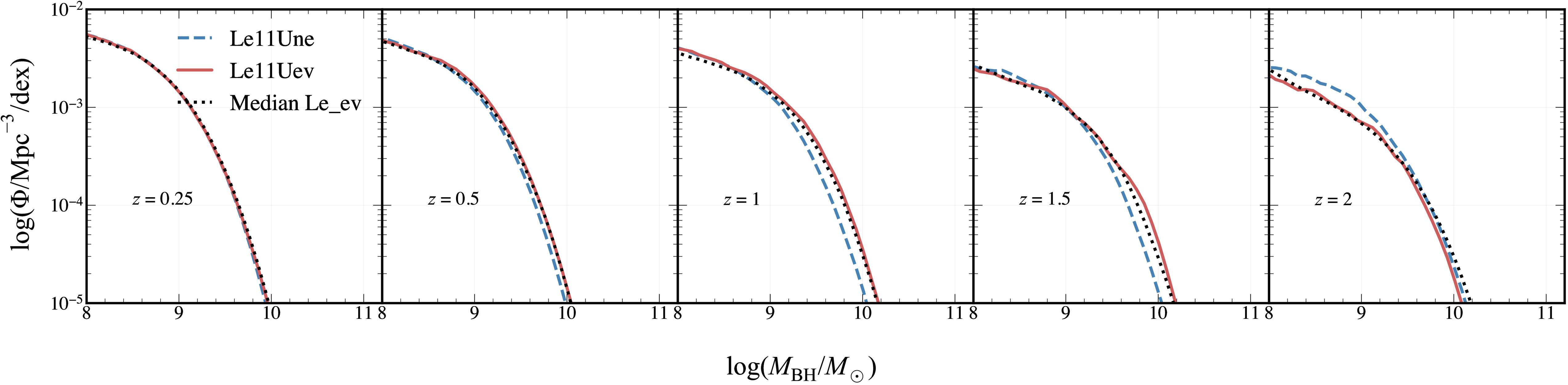
Figure 11. Refer to the following caption and surrounding text. — **Figure 11.** The posterior BHMFs associated with our two models with uniform GSMF priors. The model associated with the blue dashed line sampled only the 11 GSMF parameters, while the red solid line model additionally sampled the α_z parameter. We additionally show the posterior BHMF from Le_ne as a black dotted line. This is the same as the red solid line in Figure 7. We omit error bars for clarity, though they are slightly larger than those in Figure 7. There is broad agreement in SMBH number density across all redshift bins between the three models shown here. This demonstrates that our models have constraining power over the BHMF and are not prior dominated.
Download figure:
Standard image High-resolution image

Similar to how we tested different options for the GSMF, we additionally considered the effect of the version of the M_BH–M_bulge relation we use. In Figure 10, we demonstrate the impact of scaling relation choice on the GWB spectrum. The version of the scaling relation from J. Kormendy & L. C. Ho (2013) generally produces bigger SMBHs (and therefore higher GWB amplitudes) than other options (see, e.g., J. Simon 2023). E. R. Liepold & C.-P. Ma (2024) use the N. J. McConnell & C.-P. Ma (2013) version of the M_BH–M_bulge relation, which generally produces lower GWB amplitudes compared to that of J. Kormendy & L. C. Ho (2013). We additionally show the GWB spectrum using the scaling relation from F. Shankar et al. (2016). This comparison demonstrates that, wherever our spectra fall short of the GWB data, using a relation with a lower amplitude would only exacerbate this problem. This also has implications for our choices for the evolution we approximate for the E. R. Liepold & C.-P. Ma (2024) GSMF.

Here we demonstrate that our “direct-likelihood” method reproduces the Gaussian-process-interpolated MCMC-like methods of G. Agazie et al. (2023b). In Figure 12, we show a comparison between the posterior distributions from G. Agazie et al. (2023a) compared to our results when using the same prior model setup. We see that the two methods return negligibly different posterior distributions. The method we use in this work is also discussed in more depth in Appendix C of G. Agazie et al. (2023b).

Figure 12. Refer to the following caption and surrounding text. — **Figure 12.** Posterior distributions for the same model setup from G. Agazie et al. (2023b) when using our method (blue) vs. their (black). We find that our results are in good agreement with theirs when using the same model.
Download figure:
Standard image High-resolution image

In this work, we discovered a minor limitation of the direct-likelihood method which impacted the Le00ne model. It is more difficult for the posterior distributions to deviate from the priors because extreme values (e.g., more than 3σ above or below the prior median) have a low chance of being randomly sampled, regardless of how well that value may describe the data. We see this limitation in our model with the lowest number of sampled parameters, Le00ne. The best-fit GWB spectrum from this model returned a notably low log-likelihood compared to the other models, which means it produced a worse overall fit (see Figures 3 and 6). We can see, from Le03ev and Le00ev, that a value of α(z) > 9.0 is needed to reproduce the GWB amplitude without increasing galaxy number density. If the M_BH–M_bulge relation is not allowed to evolve, the prior for α₀ would need to be sampled at a value ≳6σ away from the prior mean (assuming a normal distribution where α₀ = 8.69 ± 0.055), making it extremely unlikely/impossible to be sampled. Without interpolating, any value that is not sampled simply does not have a corresponding GWB spectrum, and the best-fit parameters may therefore fail to describe the data. This effect can be mitigated by the choice of priors, but prior choice has its own impact on models, and so future studies should consider the impact of this effect when using this method.

It is important to emphasize that the likelihoods we calculate are a measure of how well a given best-fit spectrum describes the observed GWB spectrum, but they are not marginalized over the respective parameter spaces. This means that the likelihoods do not contain information about prior posterior agreement/disagreement, and therefore do not indicate goodness of fit to EM data. These likelihoods cannot be used alone to evaluate which models are better models of both the GWB and EM data. To evaluate consistency with EM data, we make use of other quantities such as the Kullback–Leilbler divergence, D_KL, and GSMF boost, Ξ. The “best” models have high likelihoods (good fits to the GWB) in addition to low D_KL and Ξ values (good agreement with the EM data).

We give here the full corner plots for each of our eight models (Figure 13). Note that the variables pertaining to galaxy merger rates include “GMR” in the subscript to distinguish from other parameters which use similar variables. For the parameters in the model not detailed in this paper, we refer the reader to G. Agazie et al. (2023b, and references therein) for a complete discussion. In each corner plot, the blue histograms/contours represent the posterior distributions. The priors are shown by the gray histograms.

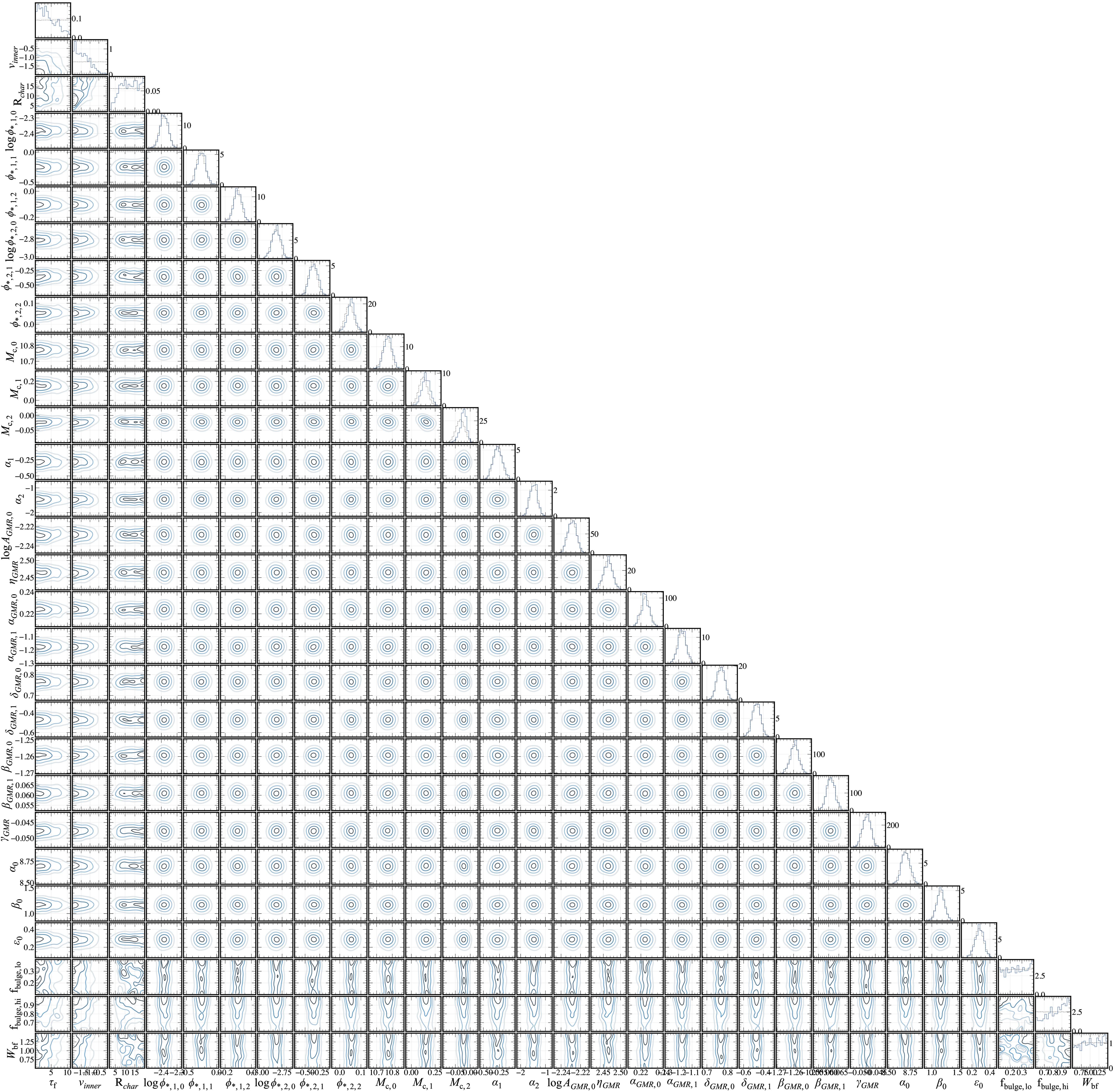
Figure 13. Refer to the following caption and surrounding text. — **Figure 13.**
The complete corner plot for Le11ne. (The complete figure set (8 images) is available.)
Download figure:
Standard image High-resolution image

Inferring MBH–Mbulge Evolution from the Gravitational-wave Background

Author notes

Author notes

Author notes

Author notes

Author notes

Author notes

Author notes

Notes

Article metrics

Share this article

Dates

Abstract

1. Introduction

2. Methods

2.1. Semi-analytic Modeling

2.2. The MBH–Mbulge Relation

2.3. The Galaxy Stellar Mass Function

2.4. The Models

3. Results

3.1. Full-sample Models

3.1.1. Le11ne and Le11ev

3.1.2. LM11ne and LM11ev

3.2. Fixed GSMF Evolution Models: Le03ne and Le03ev

3.3. Fixed GSMF Models: Le00ne and Le00ev

3.4. Influence of the GSMF

3.5. Black Hole Number Density

4. Discussion

5. Summary and Conclusions

Acknowledgments

Author Contributions

Appendix A: GSMF Evolution Parameters and Scaling Relation Choice

Appendix B: Choice of Priors and Prior Tests

Appendix C: Reliability of Methods

Appendix D: Corner Plots

Footnotes

Inferring M_BH–M_bulge Evolution from the Gravitational-wave Background

2.2. The M_BH–M_bulge Relation