Abstract
Unburned carbon is potentially a powerful probe of Type Ia supernova (SN) explosion mechanisms. We present comprehensive optical and near-infrared (NIR) data on the “transitional” Type Ia SN 2015bp. An early NIR spectrum ( days with respect to B-band maximum) displays a striking C i 1.0693 μm line at 11.9 × 10³ km s−1, distinct from the prominent Mg ii 1.0927 μm feature, which weakens toward maximum light. SN 2015bp also displays a clear C ii 6580 Å notch early (
 days) at 13.2 × 10³ km s−1, consistent with our NIR carbon detection. At
  , SN 2015bp is less luminous than a normal SN Ia and, along with iPTF 13ebh, is the second member of the transitional subclass to display prominent early-time NIR carbon absorption. We find it unlikely that the C i feature is misidentified He i 1.0830 μm because this feature grows weaker toward maximum light, while the helium line produced in some double-detonation models grows stronger at these times. Intrigued by these strong NIR carbon detections, but lacking NIR data for other SNe Ia, we investigated the incidence of optical carbon in the sample of nine transitional SNe Ia with early-time data (t ≲ −4 days). We find that four display C ii 6580 Å, while two others show tentative detections, in line with the SN Ia population as a whole. We conclude that at least ∼50% of transitional SNe Ia in our sample do not come from sub-Chandrasekhar-mass explosions due to the clear presence of carbon in their NIR and optical spectra.
1. Introduction
Type Ia supernovae (SNe Ia) are important “standardizable” candles, following a width–luminosity relationship where fainter events have faster declining light curves (Phillips 1993). Using the resulting empirically calibrated luminosities, SNe Ia have provided a direct measure of the expansion history of the universe, ultimately leading to the discovery of the accelerating expansion and “dark energy” (Riess et al. 1998; Perlmutter et al. 1999). However, supernova cosmology is currently limited by systematic errors (e.g., Conley et al. 2011; Suzuki et al. 2012; Brout et al. 2019), and further progress may mean shifting observations to the near-infrared (NIR) where SNe Ia are even better standard candles than in the optical (e.g., Krisciunas et al. 2004; Folatelli et al. 2010; Kattner et al. 2012; Avelino et al. 2019). A deeper understanding of the physics of SNe Ia is also vital both for mitigating systematic errors in future cosmology experiments and for the ultimate quest to understand the late stages of stellar evolution.
One potential, critical probe of SN Ia explosions is the incidence, quantity, and distribution of leftover carbon. There is a general consensus that SNe Ia result from the thermonuclear explosion of a carbon–oxygen white dwarf (Hoyle & Fowler 1960). Given this, carbon is the only direct probe of primordial material from the progenitor system, because oxygen is produced in carbon burning during the explosion. Specific explosion parameters and the degree of mixing are key ingredients in determining whether leftover carbon is expected for a given explosion model. For instance, the pure deflagration W7 model of Nomoto et al. (1984) leaves substantial carbon behind, while delayed-detonation models have nearly complete carbon burning for normal SNe Ia (Kasen et al. 2009), with increasing amounts of unburned carbon for fainter events (Höflich et al. 2002). Both the pulsating class of delayed-detonation models (Hoeflich et al. 1995) and violent merger models (Pakmor et al. 2012) also have a large mass fraction of carbon. The class of sub-Chandrasekhar double-detonation models, however, are characterized by the nearly complete lack of surviving carbon in recent work (e.g., Shen et al. 2018; Polin et al. 2019), although a small amount may remain below the outer layer of iron-group elements during a surface helium detonation (Fink et al. 2010). Connecting observed carbon to model expectations is of course nontrivial, but clear observational samples play an important role in distinguishing between viable SN Ia explosion mechanisms.
The identification of carbon in SNe Ia began with individual detections in normal (e.g., Branch et al. 2003; Garavini et al. 2004; Thomas et al. 2007), faint (e.g., Höflich et al. 2002; Taubenberger et al. 2008), and super-Chandrasekhar (e.g., Howell et al. 2006; Scalzo et al. 2010; Silverman et al. 2011) events, followed by several large-sample studies focused on the optical and the C ii 6580 Å feature, which appears on the red shoulder of the prominent Si ii 6355 Å absorption line (Parrent et al. 2011; Thomas et al. 2011; Folatelli et al. 2012; Silverman & Filippenko 2012; Maguire et al. 2014). In these studies, ∼20%–40% of pre-maximum spectra showed C ii features, with the fraction increasing the earlier a spectrum is taken before maximum light. In addition to this observational detection bias, it is also likely that high-velocity C ii 6580 Å is undetectable owing to the proximity and strength of the Si ii line (see, e.g., Thomas et al. 2011; Folatelli et al. 2012). There is also evidence that SNe Ia with bluer optical and ultraviolet (UV) colors are more likely to exhibit carbon features (Thomas et al. 2011; Folatelli et al. 2012; Silverman & Filippenko 2012; Milne et al. 2013), which may suggest that carbon is preferentially seen in low-metallicity progenitor systems (Heringer et al. 2017).
While most carbon studies have focused on the C ii 6580 Å line, there is observational evidence that NIR C i 1.0693 μm may be more prevalent, although the data sets are still sparse. Using the remarkable early-time and high-cadence data set for SN 2011fe, Hsiao et al. (2013) noted that the strength of the NIR C i 1.0693 μm line increased toward maximum light, and suggested this may be a consequence of the recombination of C ii to C i as the ejecta cool. Since then, several other studies have noted a similar trend for individual objects (Hsiao et al. 2015, 2019; Marion et al. 2015), although it should be noted that spectrum synthesis codes such as SYNAPPS (Thomas et al. 2011) are necessary to identify the C i 1.0693 μm line in the “shoulder” of the stronger Mg ii 1.0927 μm line for normal SNe Ia.
Perhaps the most intriguing case of NIR C i 1.0693 μm is that of iPTF 13ebh (Hsiao et al. 2015), which showed a very prominent, conspicuous absorption feature blueward of Mg ii 1.0927 μm in early-time data (t ≲ −10 days), which grew weaker toward maximum light, in contrast to the subtler appearance of C i in normal SNe Ia. iPTF 13ebh is a “transitional” SN Ia, a faint (and rare; Ashall et al. 2016a) subclass intermediate between normal and the even more subluminous SN 1991bg–like subclass. To go with their subluminous nature, transitional SNe Ia have fast decline rates (typically  –2.0 mag), but lack the strong Ti ii feature seen in SN 1991bg–like events (∼4000–4500 Å; Filippenko et al. 1992). They also exhibit an NIR primary maximum that occurs before the B-band maximum epoch and exhibit an NIR secondary maximum, again in contrast to the more underluminous SN 1991bg–like SNe Ia (Krisciunas et al. 2009). Recent modeling efforts have suggested that faint-and-fast declining SNe Ia, such as the transitional subclass, are largely produced by sub-Chandrasekhar explosions (Blondin et al. 2017; Goldstein & Kasen 2018)—in tension with the clear detection of C i in iPTF 13ebh, as carbon should be nearly nonexistent in sub-Chandrasekhar explosions. Meanwhile, abundance stratification studies of other transitional SNe Ia (SN 1986G, SN 2007on, and SN 2011iv) have been consistent with Chandrasekhar-mass delayed-detonation models (Ashall et al. 2016a, 2018). Further observational and theoretical work on transitional SNe Ia will help elucidate their progenitors and explosions.
Here we report on a second transitional SN Ia with strong early-time NIR carbon, SN 2015bp (originally studied by Srivastav et al. 2017). We also undertake an expanded search for optical carbon in the present sample of nine transitional SNe Ia with early-time data. In Section 2 we present our observations of SN 2015bp, while in Sections 3 and 4 we describe its photometric and spectroscopic properties, respectively. Section 5 discusses both the NIR and optical detection of carbon in SN 2015bp and compares it with other prominent examples in the literature. Intrigued by the strength of NIR carbon in both iPTF 13ebh and SN 2015bp, we then (Section 6) search for early optical carbon in the full sample of transitional SNe Ia in the literature. Given the incidence of both NIR and optical carbon in the transitional SN Ia subclass, we discuss the implications for various explosion models in Section 7, before concluding in Section 8.
2. Observations
2.1. Photometric Observations
SN 2015bp was discovered on (UT dates are used throughout this paper) 2015 March 16, 11:45:36 (JD = 2,457,097.99) at α(J2000) =  , δ(J2000) = +01°38′02.40″ by the Catalina Real-time Transient Survey (CRTS; Drake et al. 2009) at V = 19.2 mag, 39″ offset from the nearby S0 galaxy NGC 5839 (redshift z = 0.004069). Spectroscopically, it was initially classified as a pre-maximum SN 1991bg–like SN Ia (Jha et al. 2015), and it evolved like a normal SN Ia, except that it displayed a fast-declining light curve.
Following discovery, observations were initiated by the Carnegie Supernova Project II (CSP-II; Phillips et al. 2019; Hsiao et al. 2019), and optical photometric observations began on 2015 March 19 using the Henrietta Swope 1 m telescope at Las Campanas Observatory in Chile. The Swope observations continued until 2015 August 15, obtaining 45 epochs in the CSP-II optical Johnson (BV) and Sloan (ugri) filters. Photometry in the Swope natural system (as described by Krisciunas et al. 2017) is logged in Table 1 and the respective light curves are plotted in Figure 1. Once SN 2015bp had sufficiently faded in March 2016, host-galaxy reference images were obtained for template subtraction. All images were reduced in the manner described by Phillips et al. (2019), where point-spread function photometry of the SN (on the difference images) was computed with respect to a local sequence of stars that were calibrated to Landolt (1992) and Smith et al. (2002) standard-star fields.
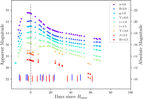
Figure 1. Optical and NIR light curves of SN 2015bp. The light-blue star represents the discovery magnitude from CRTS in the V band. The dashed line represents the time of maximum light in the B band (Table 5). The blue and red vertical lines represent epochs where optical and NIR spectra were obtained, respectively.
Download figure:
Standard image High-resolution imageTable 1. Optical Photometry of SN 2015bp in the Natural Swope System
| Date | MJD | Phase (days) | u (mag) | B (mag) | g (mag) | V (mag) | r (mag) | i (mag) |
|---|---|---|---|---|---|---|---|---|
| 2015-03-19.34 | 57100.34 | −11.38 | 16.560 ± 0.012 | 16.339 ± 0.012 | 17.435 ± 0.019 | 16.403 ± 0.008 | 16.372 ± 0.011 | 16.547 ± 0.015 |
| 2015-03-20.35 | 57101.35 | −10.37 | 15.977 ± 0.005 | 15.854 ± 0.006 | 16.645 ± 0.010 | 15.872 ± 0.005 | 15.862 ± 0.005 | 16.022 ± 0.007 |
| 2015-03-21.32 | 57102.32 | −9.40 | 15.541 ± 0.006 | 15.455 ± 0.006 | 16.019 ± 0.007 | 15.447 ± 0.005 | 15.437 ± 0.005 | 15.581 ± 0.006 |
| 2015-03-22.36 | 57103.36 | −8.36 | ... | 15.082 ± 0.013 | 15.509 ± 0.013 | 15.093 ± 0.011 | 15.057 ± 0.012 | 15.206 ± 0.018 |
| 2015-03-28.34 | 57109.34 | −2.38 | 13.966 ± 0.005 | 13.937 ± 0.005 | 14.468 ± 0.006 | 13.902 ± 0.005 | 13.893 ± 0.006 | 14.200 ± 0.005 |
| 2015-03-29.30 | 57110.30 | −1.42 | 13.941 ± 0.010 | 13.883 ± 0.009 | 14.448 ± 0.008 | 13.859 ± 0.007 | 13.838 ± 0.009 | 14.190 ± 0.010 |
| 2015-03-30.26 | 57111.26 | −0.46 | 13.899 ± 0.009 | 13.838 ± 0.008 | 14.478 ± 0.006 | 13.822 ± 0.007 | 13.808 ± 0.006 | 14.238 ± 0.009 |
| 2015-03-31.35 | 57112.35 | 0.63 | 13.886 ± 0.006 | 13.805 ± 0.006 | 14.555 ± 0.005 | 13.799 ± 0.005 | 13.800 ± 0.007 | 14.274 ± 0.007 |
| 2015-04-01.31 | 57113.31 | 1.59 | 13.892 ± 0.011 | 13.792 ± 0.010 | 14.629 ± 0.007 | 13.785 ± 0.007 | 13.738 ± 0.008 | 14.300 ± 0.008 |
| 2015-04-05.29 | 57117.29 | 5.57 | 14.134 ± 0.010 | 13.855 ± 0.007 | 15.131 ± 0.010 | 13.943 ± 0.007 | 13.870 ± 0.008 | 14.467 ± 0.011 |
| 2015-04-09.26 | 57121.26 | 9.54 | 14.582 ± 0.008 | 14.130 ± 0.008 | 15.734 ± 0.013 | 14.294 ± 0.008 | 14.199 ± 0.008 | 14.811 ± 0.009 |
| 2015-04-10.27 | 57122.27 | 10.55 | 14.725 ± 0.006 | 14.199 ± 0.007 | 15.890 ± 0.009 | 14.413 ± 0.008 | 14.273 ± 0.009 | 14.852 ± 0.010 |
| 2015-04-11.29 | 57123.29 | 11.57 | 14.874 ± 0.007 | 14.280 ± 0.006 | 16.056 ± 0.009 | 14.535 ± 0.008 | 14.310 ± 0.006 | 14.842 ± 0.007 |
| 2015-04-13.32 | 57125.32 | 13.60 | 15.166 ± 0.010 | 14.455 ± 0.008 | 16.413 ± 0.014 | 14.771 ± 0.006 | 14.372 ± 0.005 | 14.798 ± 0.007 |
| 2015-04-14.29 | 57126.29 | 14.57 | 15.310 ± 0.007 | 14.521 ± 0.006 | 16.552 ± 0.015 | 14.903 ± 0.006 | 14.400 ± 0.006 | 14.767 ± 0.011 |
| 2015-04-17.24 | 57129.24 | 17.52 | 15.704 ± 0.010 | 14.779 ± 0.007 | 16.994 ± 0.015 | 15.301 ± 0.006 | 14.513 ± 0.006 | 14.725 ± 0.009 |
| 2015-04-18.27 | 57130.27 | 18.55 | 15.833 ± 0.008 | 14.863 ± 0.006 | 17.106 ± 0.013 | 15.414 ± 0.005 | 14.554 ± 0.005 | 14.713 ± 0.006 |
| 2015-04-19.31 | 57131.31 | 19.59 | 15.956 ± 0.010 | 14.959 ± 0.006 | 17.196 ± 0.014 | 15.526 ± 0.007 | 14.626 ± 0.008 | 14.715 ± 0.010 |
| 2015-04-20.28 | 57132.28 | 20.56 | 16.052 ± 0.010 | 15.058 ± 0.009 | 17.288 ± 0.015 | 15.638 ± 0.006 | 14.707 ± 0.005 | 14.762 ± 0.007 |
| 2015-04-22.32 | 57134.32 | 22.6 | 16.242 ± 0.009 | 15.247 ± 0.006 | 17.431 ± 0.014 | 15.831 ± 0.006 | 14.908 ± 0.006 | 14.916 ± 0.006 |
| 2015-04-23.33 | 57135.33 | 23.61 | 16.339 ± 0.009 | 15.346 ± 0.009 | 17.488 ± 0.016 | 15.930 ± 0.007 | 15.014 ± 0.006 | 15.016 ± 0.007 |
| 2015-04-24.31 | 57136.31 | 24.59 | 16.420 ± 0.010 | 15.427 ± 0.007 | 17.565 ± 0.013 | 15.992 ± 0.006 | 15.105 ± 0.008 | 15.107 ± 0.008 |
| 2015-04-25.27 | 57137.27 | 25.55 | 16.466 ± 0.011 | 15.502 ± 0.010 | 17.629 ± 0.016 | 16.051 ± 0.008 | 15.191 ± 0.010 | 15.195 ± 0.010 |
| 2015-04-26.26 | 57138.26 | 26.54 | 16.524 ± 0.008 | 15.556 ± 0.007 | 17.688 ± 0.014 | 16.122 ± 0.005 | 15.268 ± 0.005 | 15.285 ± 0.007 |
| 2015-04-27.25 | 57139.25 | 27.53 | 16.570 ± 0.008 | 15.625 ± 0.006 | 17.735 ± 0.013 | 16.175 ± 0.007 | 15.333 ± 0.005 | 15.358 ± 0.007 |
| 2015-04-28.24 | 57140.24 | 28.52 | 16.603 ± 0.008 | 15.678 ± 0.006 | 17.810 ± 0.013 | 16.231 ± 0.006 | 15.408 ± 0.006 | 15.423 ± 0.008 |
| 2015-04-30.26 | 57142.26 | 30.54 | 16.692 ± 0.011 | 15.775 ± 0.009 | 17.870 ± 0.019 | 16.321 ± 0.009 | 15.518 ± 0.007 | 15.562 ± 0.009 |
| 2015-05-02.24 | 57144.24 | 32.52 | 16.795 ± 0.013 | 15.869 ± 0.007 | 17.914 ± 0.027 | 16.383 ± 0.007 | 15.624 ± 0.007 | 15.672 ± 0.006 |
| 2015-05-06.30 | 57148.30 | 36.58 | 16.889 ± 0.014 | 16.000 ± 0.010 | 18.027 ± 0.034 | 16.509 ± 0.009 | 15.812 ± 0.008 | 15.888 ± 0.008 |
| 2015-05-09.26 | 57151.26 | 39.54 | 16.960 ± 0.011 | 16.089 ± 0.007 | 18.122 ± 0.023 | 16.598 ± 0.006 | 15.930 ± 0.005 | 16.006 ± 0.006 |
| 2015-05-11.26 | 57153.26 | 41.54 | 17.024 ± 0.011 | 16.177 ± 0.009 | 18.166 ± 0.016 | 16.655 ± 0.009 | 16.018 ± 0.009 | 16.125 ± 0.010 |
| 2015-05-13.25 | 57155.25 | 43.53 | 17.079 ± 0.011 | 16.241 ± 0.012 | 18.251 ± 0.017 | 16.712 ± 0.008 | 16.099 ± 0.010 | 16.225 ± 0.013 |
| 2015-05-15.24 | 57157.24 | 45.52 | 17.127 ± 0.011 | 16.306 ± 0.008 | 18.314 ± 0.024 | 16.758 ± 0.012 | 16.130 ± 0.009 | 16.311 ± 0.009 |
| 2015-05-17.28 | 57159.28 | 47.56 | 17.153 ± 0.009 | 16.358 ± 0.007 | 18.340 ± 0.017 | 16.816 ± 0.007 | 16.246 ± 0.008 | 16.378 ± 0.010 |
| 2015-05-19.25 | 57161.25 | 49.53 | 17.217 ± 0.009 | 16.421 ± 0.009 | 18.453 ± 0.021 | 16.858 ± 0.009 | 16.318 ± 0.010 | 16.453 ± 0.013 |
| 2015-05-21.24 | 57163.24 | 51.52 | 17.250 ± 0.008 | 16.470 ± 0.009 | 18.468 ± 0.017 | 16.878 ± 0.007 | 16.393 ± 0.006 | 16.558 ± 0.008 |
| 2015-05-24.20 | 57166.20 | 54.48 | 17.309 ± 0.009 | 16.554 ± 0.008 | 18.543 ± 0.017 | 16.967 ± 0.006 | 16.516 ± 0.006 | 16.677 ± 0.009 |
| 2015-06-03.20 | 57176.20 | 64.48 | 17.562 ± 0.027 | 16.834 ± 0.015 | 18.922 ± 0.071 | 17.177 ± 0.014 | 16.880 ± 0.011 | 17.049 ± 0.014 |
| 2015-06-05.23 | 57178.23 | 66.51 | 17.540 ± 0.024 | 16.893 ± 0.015 | 18.928 ± 0.049 | 17.189 ± 0.012 | 16.961 ± 0.011 | 17.139 ± 0.015 |
| 2015-06-06.23 | 57179.23 | 67.51 | 17.530 ± 0.023 | 16.909 ± 0.015 | 19.077 ± 0.148 | 17.218 ± 0.015 | 17.013 ± 0.013 | 17.176 ± 0.016 |
| 2015-06-08.19 | 57181.19 | 69.47 | 17.570 ± 0.010 | 16.996 ± 0.009 | 18.945 ± 0.029 | 17.247 ± 0.008 | 17.081 ± 0.009 | 17.265 ± 0.011 |
| 2015-06-09.19 | 57182.19 | 70.47 | 17.595 ± 0.011 | 16.982 ± 0.007 | 19.059 ± 0.026 | 17.265 ± 0.007 | 17.109 ± 0.007 | 17.272 ± 0.010 |
| 2015-08-15.03 | 57249.03 | 137.31 | 18.791 ± 0.014 | 18.616 ± 0.018 | 20.877 ± 0.122 | 18.569 ± 0.012 | 19.250 ± 0.027 | 19.072 ± 0.031 |
Note. The phase is with respect to the time of B-band maximum.
Download table as: ASCIITypeset image
Retrocam on the du Pont 2.5 m telescope located at Las Campanas Observatory was also used to obtain 11 epochs of NIR photometric data in the YJH filters starting on 2015 March 28 and ending on 2015 May 30. These observations are logged in Table 2. The images were reduced as described by Contreras et al. (2010). The JH bands were both calibrated using the Persson et al. (1998) system of standard stars. The Y band was calibrated using a set of Persson standards as described by Krisciunas et al. (2017).
Table 2. NIR Photometry of SN 2015bp
| Date | MJD | Phase (days) | Y (mag) | J (mag) | H (mag) |
|---|---|---|---|---|---|
| 2015-03-28.34 | 57109.34 | −2.38 | 14.024 ± 0.005 | 13.975 ± 0.005 | 14.106 ± 0.005 |
| 2015-03-30.26 | 57111.26 | −0.46 | 14.055 ± 0.005 | 13.984 ± 0.005 | 14.134 ± 0.005 |
| 2015-03-31.35 | 57112.35 | 0.63 | ⋯ | 14.040 ± 0.005 | 14.201 ± 0.005 |
| 2015-04-01.31 | 57113.31 | 1.59 | ⋯ | 14.105 ± 0.008 | 14.259 ± 0.005 |
| 2015-04-02.27 | 57114.27 | 2.55 | 14.270 ± 0.006 | 14.208 ± 0.005 | 14.309 ± 0.006 |
| 2015-04-03.30 | 57115.30 | 3.58 | 14.350 ± 0.007 | 14.300 ± 0.007 | 14.356 ± 0.007 |
| 2015-04-08.26 | 57120.26 | 8.54 | 14.662 ± 0.005 | 15.195 ± 0.005 | 14.527 ± 0.005 |
| 2015-04-25.27 | 57137.27 | 25.55 | 14.206 ± 0.005 | 15.367 ± 0.005 | 14.725 ± 0.005 |
| 2015-04-29.21 | 57141.21 | 29.49 | 14.488 ± 0.007 | 15.832 ± 0.009 | 15.050 ± 0.007 |
| 2015-05-02.24 | 57144.24 | 32.52 | 14.703 ± 0.005 | 16.138 ± 0.007 | 15.224 ± 0.007 |
| 2015-05-28.18 | 57170.18 | 58.46 | 16.265 ± 0.007 | 18.187 ± 0.034 | 16.526 ± 0.020 |
| 2015-05-30.17 | 57172.17 | 60.45 | 16.383 ± 0.008 | 18.325 ± 0.034 | 16.637 ± 0.016 |
Note. Phase is with respect to B-band maximum.
Download table as: ASCIITypeset image
2.2. Spectroscopic Observations
Optical spectroscopic observations began on 2013 March 20 and were made with the low-resolution EFOSC2 spectrograph on the 3.6 m New Technology Telescope (NTT), the Wide-Field Reimaging CCD Camera (WFCCD) on the du Pont 100 inch telescope, the Deep Imaging Multi-Object Spectrograph (DEIMOS; Faber et al. 2003) on the Keck II 10 m telescope, and the Andalucia Faint Object Spectrograph and Camera (ALFOSC) on the Nordic Optical Telescope (NOT). The optical spectroscopic observations are logged in Table 3 and displayed in Figure 2. We also include some already published spectra from Srivastav et al. (2017), which help fill in the post-maximum evolution. The EFOSC2 data were taken as part of the Public ESO Spectroscopic Survey of Transient Objects (PESSTO) project (Smartt et al. 2015), and the reduced spectra were downloaded directly from the ESO archive.

Figure 2. Optical spectral evolution of SN 2015bp. Labels are displayed in days relative to  .(The data used to create this figure are available.)
Download figure:
Standard image High-resolution imageTable 3. Journal of Optical Spectroscopic Observations
| UT Date | MJD | Instrument |
 a
a
|
 b
b
|
|---|---|---|---|---|

|

| |||
| 2015-03-20.32 | 57101.3 | EFOSC | −10.9 | 45.0 |
| 2015-03-27.16 | 57108.2 | ALFOSC | −4.1 | 25.0 |
| 2015-03-28.38 | 57109.4 | EFOSC | −2.8 | 10.0 |
| 2015-03-31.00 | 57112.0 | HFOSC | −0.2 | c |
| 2015-04-02.00 | 57114.0 | HFOSC | 1.8 | c |
| 2015-04-03.00 | 57115.0 | HFOSC | 2.8 | c |
| 2015-04-05.00 | 57117.0 | HFOSC | 4.8 | c |
| 2015-04-10.34 | 57122.3 | EFOSC | 10.1 | 10.0 |
| 2015-04-13.11 | 57125.1 | ALFOSC | 12.9 | 30.0 |
| 2015-04-19.22 | 57131.2 | EFOSC | 19.0 | 15.0 |
| 2015-04-24.32 | 57136.3 | WFCCD | 24.1 | 10.0 |
| 2015-05-12.03 | 57154.0 | ALFOSC | 41.8 | 30.0 |
| 2015-05-20.40 | 57162.4 | DEIMOS | 50.2 | 15.0 |
| 2015-07-19.03 | 57222.0 | WFCCD | 109.8 | 16.7 |
| 2015-08-14.90 | 57248.9 | ALFOSC | 136.7 | 40.0 |
| 2015-09-15.98 | 57281.0 | EFOSC | 168.8 | 45.0 |
Notes.
a is the time relative to
  , in days.
b
, in days.
b
 is the total integration time in minutes.
c
Data from the HFOSC instrument were published in Srivastav et al. (2017) and were acquired from https://sne.space. They did not include exposure times in their publication.
is the total integration time in minutes.
c
Data from the HFOSC instrument were published in Srivastav et al. (2017) and were acquired from https://sne.space. They did not include exposure times in their publication.Download table as: ASCIITypeset image
NIR spectroscopic observations began on 2015 March 21 using the Son of ISAAC (SOFI) instrument on the NTT (Moorwood et al. 1998), the Folded-port Infrared Echellette (FIRE; Simcoe et al. 2013) spectrograph on the Magellan Baade telescope, the Gemini Near Infrared Spectrograph (GNIRS; Elias et al. 1998) on the Gemini North Telescope, SpeX (Rayner et al. 2003) on the NASA Infrared Telescope Facility (IRTF), and the Flamingos2 spectrograph (F2; Eikenberry et al. 2006) on the Gemini South Telescope. These observations are logged in Table 4 and displayed in Figure 3. The SOFI data were taken during the PESSTO survey (Smartt et al. 2015), and we downloaded the reduced spectra directly from the ESO archive. The FIRE, GNIRS, and F2 spectroscopic data were reduced in the manner described by Hsiao et al. (2019).

Figure 3. NIR spectral evolution of SN 2015bp. Labels are displayed relative to  .(The data used to create this figure are available.)
Download figure:
Standard image High-resolution imageTable 4. Journal of NIR Spectroscopic Observations
| UT Date | MJD | Instrument |
 a
a
|
 b
b
|
|---|---|---|---|---|

|

| |||
| 2015-03-21.27 | 57102.3 | SOFI | −9.9 | 36.0 |
| 2015-03-23.40 | 57104.4 | F2 | −7.8 | 17.5 |
| 2015-03-29.31 | 57110.3 | SOFI | −1.9 | 36.0 |
| 2015-04-02.36 | 57114.4 | FIRE | 2.1 | 8.4 |
| 2015-04-07.29 | 57119.3 | FIRE | 7.1 | 8.4 |
| 2015-04-12.22 | 57124.2 | FIRE | 12.0 | 8.4 |
| 2015-04-16.41 | 57128.4 | GNIRS | 16.2 | 20.0 |
| 2015-04-19.38 | 57131.4 | IRTF | 19.2 | 47.4 |
| 2015-04-23.23 | 57135.2 | GNIRS | 23.0 | 24.0 |
| 2015-05-07.36 | 57149.4 | GNIRS | 37.2 | 35.0 |
| 2015-05-17.37 | 57159.4 | IRTF | 47.2 | 49.9 |
| 2015-06-01.21 | 57174.2 | FIRE | 62.0 | 21.1 |
Notes.
a is the time relative to
  in days.
b
in days.
b
 is the total integration time in minutes.
Download table as: ASCIITypeset image
Once all the spectra were reduced in their respective manners, they were flux-scaled to match the photometry. We also accounted for the Milky Way extinction given an  mag color excess (Schlafly & Finkbeiner 2011) with RV
= 3.1, and the redshift of the host galaxy (z = 0.004069 ± 0.000017) by shifting the wavelength of the spectra to their rest frame. We do not correct for any further host-galaxy extinction (consistent with Srivastav et al. 2017).
mag color excess (Schlafly & Finkbeiner 2011) with RV
= 3.1, and the redshift of the host galaxy (z = 0.004069 ± 0.000017) by shifting the wavelength of the spectra to their rest frame. We do not correct for any further host-galaxy extinction (consistent with Srivastav et al. 2017).
3. Photometric Properties
Optical light-curve data (BVugri) were obtained for SN 2015bp from  days with respect to
  to roughly 137 days afterward, whereas the NIR data (YJH) span
  to 60 days. These data are plotted in Figure 1 up to day ∼70. All of the data are logged in Tables 1 and 2.
We fit the light curve using the SNooPy software package (Burns et al. 2011, with  km s−1 Mpc−1 to calibrate the Phillips relation), and we tabulate the results in Table 5. SN 2015bp reached
  on JD 2,457,112.72 with an apparent magnitude of
  after applying reddening corrections due to foreground Milky Way extinction. SNooPy infers a distance modulus of
  mag and an absolute magnitude of
  mag.
mag.
Table 5. Basic Properties of SN 2015bp
| α(J2000) |

|
| δ(J2000) |

|
JD a
a
| 2,457,093.64 ± 1.68 |
JD
| 2,457,097.99 |
JD
|

|

| 13.69 ± 0.01 mag |
 b
,
c
b
,
c
| –18.46 ± 0.41 mag |

| 1.56 ± 0.03 mag |
| sBV | 0.671 ± 0.030 |
| Host | NGC 5839 |
| Heliocentric redshift d | 0.004069 ± 0.000017 |
| Distance modulus e | 32.15 ± 0.40 mag |
| Distance modulus f | 32.426 ± 0.088 mag |

| 0.0465 ± 0.0004 mag |
Notes.
a Derived from the fit of the power law of Piro & Nakar (2013) to the Si ii 6355 Å velocity time evolution.
b
Peak magnitudes include a reddening correction for foreground Milky Way extinction.
c
Absolute magnitude calculated using the distance modulus from the mean Tully–Fisher relation.
d
Cappellari et al. (2011).
e
Distance modulus estimated using the mean Tully–Fisher relation from Theureau et al. (2007).
f
Distance modulus estimated using SNooPy (Burns et al. 2014).
power law of Piro & Nakar (2013) to the Si ii 6355 Å velocity time evolution.
b
Peak magnitudes include a reddening correction for foreground Milky Way extinction.
c
Absolute magnitude calculated using the distance modulus from the mean Tully–Fisher relation.
d
Cappellari et al. (2011).
e
Distance modulus estimated using the mean Tully–Fisher relation from Theureau et al. (2007).
f
Distance modulus estimated using SNooPy (Burns et al. 2014).Download table as: ASCIITypeset image
There is an existing Tully–Fisher-based distance measurement to NGC 5839 corresponding to μ = 32.1 ± 0.40 mag (Theureau et al. 2007), which if applied would yield  mag. For this paper, we use the Tully–Fisher-based distance modulus and absolute magnitude hereafter, and note that if we adopt the SNoopy distance we would obtain a similar absolute magnitude to within the uncertainties.
Further, we measure a decline rate of  mag and color-stretch parameter
  . The color-stretch parameter in particular is a better way of characterizing the light curve for fast-declining SNe Ia (see Burns et al. 2014), because the linear decline in the B-band occurs earlier than +15 days for fast-declining SNe, and the MB
versus
. The color-stretch parameter in particular is a better way of characterizing the light curve for fast-declining SNe Ia (see Burns et al. 2014), because the linear decline in the B-band occurs earlier than +15 days for fast-declining SNe, and the MB
versus  relation bifurcates in this region. Using the sBV
parameter leads to the fastest declining events appearing as a continuous tail end of the normal SN Ia population (see, e.g., Burns et al. 2018; Gall et al. 2018).
relation bifurcates in this region. Using the sBV
parameter leads to the fastest declining events appearing as a continuous tail end of the normal SN Ia population (see, e.g., Burns et al. 2018; Gall et al. 2018).
We recognize that our measured value of  is smaller than what Srivastav et al. (2017) report in their study of SN 2015bp. In Figure 4 we show a comparison of the CSP-II B-band light curve (around the time of
  ) compared to the photometry reported by Srivastav et al. (2017). Assuming that the B-band light curve of Srivastav et al. (2017) is on the standard filter system, the S-correction to the Swope natural system is at the 1% level and does not account for the discrepancy observed. They report a
  value at 1.72 mag, whereas ours is at 1.56 mag. We performed a direct low-order polynomial fit to the Srivastav et al. (2017) B-band data, which yielded
  mag. Despite the discrepancy, both values are consistent with light-curve decline rates for transitional SNe Ia. The data in the current work better sampled the light curve around maximum light and at earlier phases, both of which make us confident in our measurements.

Figure 4. Comparison of the B-band photometry from Srivastav et al. (2017) and the CSP-II B photometry for SN 2015bp, displaying the discrepancy in  . A spline fit to the CSP-II B data is plotted to guide the eye.
Download figure:
Standard image High-resolution imageTransitional SNe Ia have the characteristic that they reach primary NIR maxima slightly prior to their  (as discussed in Hsiao et al. 2015). Examining the NIR light curves for SN 2015bp, there is evidence that it does exhibit the “transitional” characteristic of having its primary NIR peak before tmax(B) along with a secondary peak. This is evident primarily in the i and Y bands.
4. Spectroscopic Properties
4.1. Optical Properties
As illustrated in Figure 2, SN 2015bp is clearly an SN Ia, displaying strong absorption features of ionized intermediate-mass and iron-peak elements (Si ii, Ca ii, Fe ii, Mg i, etc), and lacking helium and hydrogen features. In this section we go over the broad spectroscopic properties of SN 2015bp, although we will largely avoid repeating the analysis already presented by Srivastav et al. (2017), before focusing on the prominent NIR and optical carbon features and their consequences.
In Figure 5 we compare SN 2015bp with several other prominent SNe Ia at both pre-maximum and maximum light epochs
16
: iPTF 13ebh, a transitional SN Ia (Hsiao et al. 2015); SN 2011fe, a normal SN Ia (Pereira et al. 2013; Maguire et al. 2014); SN 2007on, another transitional SN Ia (Folatelli et al. 2013; Gall et al. 2018); SN 1991bg, the prototypical subluminous SN Ia (Filippenko et al. 1992); and SN 1999by, another SN 1991bg–like SN Ia (Höflich et al. 2002; Garnavich et al. 2004). Underluminous and transitional SNe Ia, in particular, have several spectroscopic features that distinguish them from normal and SN 1991bg–like events. First, the O i 7774 Å absorption feature is more prominent in both classes of underluminous SNe Ia than in normal objects like SN 2011fe (e.g., Taubenberger et al. 2008; Taubenberger 2017, and see Figure 5). The relative strength of the Si ii 5972 Å feature is greater in subluminous SNe Ia than in normal objects as well, and they are generally classified as “cool” (CL) events in the Branch et al. (2006) classification scheme. To quantify this, we find pseudo-equivalent width values for Si ii 5972 Å and 6355 Å of ≈35 Å and ≈108 Å, respectively, in our spectrum taken  days before the time of B maximum. Other transitional SNe Ia, such as iPTF 13ebh and SN 2007on, also belong to the CL subclass. An Mg ii or Fe iii feature at ∼4200 Å is relatively strong in transitional SNe Ia compared to normal SNe Ia (Hsiao et al. 2015), while a Ti ii “trough” stands out in SN 1991bg–like SNe Ia in roughly the same wavelength range. Qualitatively, SN 2015bp is a clear transitional SN Ia, displaying all of these spectroscopic hallmarks, and is remarkably similar to iPTF 13ebh.
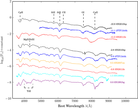
Figure 5. Comparison of optical spectra of SN 2015bp with those of other notable SNe Ia at both pre-maximum and near-maximum light phases. Absorption features discussed in the text are noted.
Download figure:
Standard image High-resolution imageThe Si ii 6355 Å absorption feature is ubiquitous in SNe Ia and is often used to measure the photospheric velocity of the SN ejecta. In Figure 6 we display a plot of Si ii velocity versus phase in comparison to other SNe Ia. The error associated with each velocity value was calculated by taking the minimum Si ii absorption wavelength value and calculating the velocity at ±2 Å from the minimum values, and propagating it through the relativistic Doppler equation as done by Silverman et al. (2012). We find that the velocity time evolution of SN 2015bp follows closely that of iPTF 13ebh. Since the velocity at around the time of  is ∼10,600 km s−1, SN 2015bp would be placed into the normal-velocity (NV) subclass as described by Wang et al. (2009).
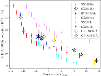
Figure 6. Si ii 6355 Å velocity comparison for SN 2015bp and other SNe Ia. We also plot the C ii 6580 Å and C i 10693 Å velocities for SN 2015bp.
Download figure:
Standard image High-resolution imageWe constrained the explosion epoch by fitting the Si ii 6355 Å velocity time evolution to a  power law. As proposed by Piro & Nakar (2013), this velocity-inferred explosion time may indicate that the supernova had a “dark phase” during the period prior to when the heating from 56Ni first reaches the outer ejecta. This analysis implies an explosion epoch 19.08 ± 1.68 days prior to
  (JD = 2,457,093.64), where the uncertainties are inferred by calculating the explosion epoch assuming both
  and
and  (see Piro & Nakar 2013). This gives us a potential dark phase of 4.3 days prior to CRTS discovery (JD = 2,457,097.9), although since no detection limits are available, this dark phase should be considered an upper limit. Given this, we note in passing that iPTF 13ebh had an inferred dark phase of ∼4 days, so our limit is plausible.
4.2. NIR Properties
We also present the full NIR spectroscopic evolution of SN 2015bp in Figure 3, spanning from roughly 10 days before through 60 days past maximum light. We will continue our discussion of the C i 1.0693 μm feature in the next section, but here we present a qualitative NIR spectroscopic comparison of SN 2015bp with the transitional SN iPTF 13ebh (Hsiao et al. 2015) and SN 1991bg–like SN 1999by (Höflich et al. 2002), along with the two normal and well-studied SNe Ia, SN 2011fe (Hsiao et al. 2013) and SN 2014J (Marion et al. 2015)—see Figure 7. One can see that at the earliest epochs, both SN 2015bp and iPTF 13ebh display a strong absorption feature blueward of the Mg ii 1.0927 μm line, which we identify as C i 1.0693 μm, and discuss further in Section 5. No such feature is seen in the comparison for normal SNe Ia, and while we do not have an early-time SN 1991bg–like comparison spectrum, we do see a strong absorption feature blueward of Mg ii in the maximum-light spectrum of SN 1999by, which has been interpreted as C i 1.0693 μm as well (Höflich et al. 2002; Hsiao et al. 2015). The strong carbon feature is weak in the transitional SNe Ia at maximum light, although there is still a faint feature in SN 2015bp, which we mark in Figure 7. The broad, asymmetric blue wing of the Mg ii 1.0927 μm absorption feature in SNe 2011fe and 2014J has also been presented as evidence for C i 1.0693 μm in those events (Hsiao et al. 2013; Marion et al. 2015).

Figure 7. Comparison of NIR spectra of SN 2015bp with those of other notable SNe Ia at both pre-maximum and near-maximum light phases. Absorption features discussed in the text are noted.
Download figure:
Standard image High-resolution imageThe emission feature (and accompanying weak absorption feature blueward of it) at ∼1.25 μm has previously been identified with Si iii 1.2523, 1.2601 μm (Hsiao et al. 2019). While clearly seen in both the transitional and normal SNe Ia at maximum light, there is no similar feature in the SN 1991bg–like SN 1999by. This absence may be real and due to the “cool,” low-temperature nature of this subclass of SNe Ia, or it may be a consequence of the lower-quality data available for SN 1999by. Further observations of SN 1991bg–like SNe Ia in the NIR are necessary.
Another region of NIR spectroscopic interest coincides with the H band where, between maximum light and ∼+10 days, this region hosts a complex iron-peak emission feature that originates from allowed transitions above the photosphere (Wheeler et al. 1998; Höflich et al. 2002; Marion et al. 2009; Hsiao et al. 2013). This feature can provide a constraint on the amount of 56Ni, considering it consists of a blend of many Fe ii/Co ii/Ni ii emission lines, which are produced through the radioactive decay of 56Ni. The study by Ashall et al. (2019a) revealed a correlation between the light-curve shape and velocity ( ) of the edge of the H feature, confirming a result from Hsiao et al. (2013). The measurement of
  corresponds to the transition in the ejecta between complete and incomplete Si-burning regions, and is determined by the exchange between the mass of 56Ni and the intermediate-mass elements formed in the explosion. Their work included NIR spectra of SN 2015bp (labeled SNHunt281 in their study) and showed that the measurement of
  for its feature is ∼−12,000
  , which is consistent with the other transitional SNe Ia in their sample.
5. Carbon Detections and Comparisons
In this section we discuss the likely detection of carbon in SN 2015bp, particularly the strong C i 1.0693 μm line, with respect to other SN Ia measurements in the literature.
We first put SN 2015bp in context with another transitional SNe Ia, iPTF 13ebh, and the SN 1991bg–like SN 1999by. We plot a time sequence around the optical C ii 6580 Å and NIR C i 1.0693 μm lines for all three SNe in Figure 8. Both SN 2015bp and iPTF 13ebh show a distinct absorption feature blueward of the Mg ii 1.0927 μm line, which grows weaker toward maximum light. If this line is C i 1.0693 μm, it would be at the photospheric velocity (see Figures 6 and 8). SN 2015bp also shows a clear C ii 6580 Å notch that grows weaker toward maximum light, while iPTF 13ebh has a “flat” morphology on the red shoulder of Si ii in the earliest spectrum, which is often recognized as a tentative C ii detection (see, e.g., Folatelli et al. 2012; Silverman & Filippenko 2012). Indeed, direct SYNAPPS modeling of iPTF 13ebh indicates that this “flat” feature is weak C ii (Hsiao et al. 2015). By contrast, SN 1999by displays an apparently strong C i 1.0693 μm feature up through maximum light and beyond (although no early-time data are available), staying roughly the same strength throughout. There is a “flat” detection of C ii 6580 Å as well, although we do not have data at early phases when C ii detections are more likely (e.g., Parrent et al. 2011).
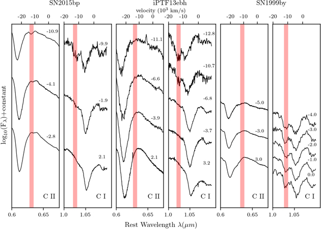
Figure 8. Comparison of the optical C ii and NIR C i evolution of SN 2015bp with that of iPTF 13ebh (another transitional SN Ia) and SN 1999by (an SN 1991bg–like SN Ia). Timescales are given in days relative to  . The red bar marks the photospheric velocity (as determined by the Si ii velocity) for the first epoch of observations for a given SN, and is only meant to guide the eye. Both SN 2015bp and iPTF 13ebh show early, strong C i that grows weaker with time. SN 2015bp also shows optical C ii absorption, while iPTF 13ebh shows a “flat” spectral feature at early times, which may also be C ii but is more ambiguous. Early-time data are not available for SN 1999by, but it shows a prominent absorption feature where one would expect C i, although it remains strong through maximum light, in contrast to the transitional SNe Ia. SN 1999by also shows a flat feature where C ii would be expected.
Download figure:
Standard image High-resolution imageIn Figure 9 we attempt to locate other, weak carbon features in SN 2015bp. In the optical, the only clearly visible feature is the standard 6580 Å absorption line, although there is a weak notch that may be associated with C ii 0.7234 μm in our −10.9 days spectrum. No C i absorption at 1.1754 μm or 1.4543 μm is apparent, and we note that we have effectively no data to identify the C i 0.9093 μm and 0.9406 μm features.
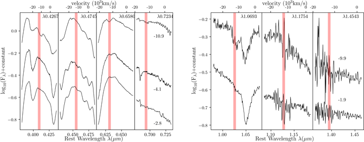
Figure 9. Optical and NIR carbon lines in SN 2015bp. We highlight the region around optical C ii and NIR C i lines beyond the standard C ii 6580 Å and NIR C i 1.0693 μm features typically identified. The panel on the left shows the three earliest optical spectra and the panel on the right displays the earliest NIR spectra (all phases with respect to  ). The red bar marks the photospheric velocity at −10.9 days, and is only meant to guide the eye. The NIR data are generally too noisy to see any features beyond C i 1.0693 μm. There may be a weak detection of C ii 0.7234 μm in the −10.9 days optical spectrum, but otherwise no clear carbon features are apparent.
Download figure:
Standard image High-resolution imageWe investigate the extent of carbon burning by comparing the Doppler velocities of the C ii 6580 Å line and the strong Si ii 6355 Å absorption feature (see, e.g., Parrent et al. 2011), which is typically used as a proxy for the photospheric velocity. We display the results in Table 6. v(C ii λ6580)/v(Si ii λ6355) is near unity, with an average value of ∼1.02, which stays constant for the ∼8 days over which we can make these measurements (from −10.9 to −2.8 days with respect to B maximum). In their much larger samples of SNe Ia, other analyses have also found roughly constant values of v(C ii λ6580)/v(Si ii λ6355), with a value slightly above unity (Parrent et al. 2011; Silverman & Filippenko 2012). This consistency among SNe Ia, with very few deviations, has been used as evidence that carbon is distributed in a layered (or hemispheric) geometry. A clumpy distribution will inevitably be seen at arbitrary orientations, and thus lead to some values of v(C ii λ6580)/v(Si ii λ6355) < 1 (Parrent et al. 2011).
Table 6. SN 2015bp Velocity Measurements for C ii (6580 Å), C i (1.0693 μm), and Si ii (6355 Å)
| tmax(B) |

|

|

|

|
|---|---|---|---|---|

| (103 km s−1) | (103 km s−1) | (103 km s−1) | |
| −10.9 | 13.2 ± 0.2 | ⋯ | 13.0 ± 0.1 | 1.03 ± 0.02 |
| −9.9 | ⋯ | 11.9 ± 0.3 | ⋯ | ⋯ |
| −4.1 | 11.8 ± 0.3 | ⋯ | 11.5 ± 0.1 | 1.02 ± 0.03 |
| −2.8 | 11.5 ± 0.3 | ⋯ | 11.3 ± 0.1 | 1.02 ± 0.03 |
| −1.9 | ⋯ | 11.4 ± 0.4 | ⋯ | ⋯ |
| 2.1 | ⋯ | 11.1 ± 0.5 | ⋯ | ⋯ |
Note. We also include the ratio of the C ii and Si ii velocities for coincident measurements. Times are measured in days relative to  , and velocities are in units of 103 km s−1.
Download table as: ASCIITypeset image
We also measured the Doppler velocities of the NIR C i 1.0693 μm line, as seen and reported in Table 6. Since the NIR C i feature is blended heavily with the Mg ii 1.0927 μm absorption feature, its velocity was measured by fitting a multicomponent Gaussian and measuring the C i feature at the minimum of its respective Gaussian. The velocities of the C i and C ii features largely track each other with phase, although the earliest measurements display a ∼1000 km s−1 difference, which is roughly the size of our measurement uncertainties. This indicates that the C i and C ii are coming from the same layer of the SN ejecta.
Finally, we zoom in on the C i 1.0693 μm feature for a sample of SNe Ia with early NIR spectra (t ≲ −10 days) in Figure 10. The sequence is plotted as a function of  and shows a clear trend of stronger C i for intrinsically fainter (and faster declining) SNe Ia. In particular, transitional SNe Ia such as iPTF 13ebh and SN 2015bp have distinct C i absorption features at early times, while normal SNe Ia are more ambiguous. There is an extended “blue shoulder” apparent in the Mg ii line for all of the normal SNe Ia, which has been interpreted (via SYNAPPS modeling) as weak C i (see, e.g., Hsiao et al. 2013, 2015; Marion et al. 2015), which if true would imply a continuous sequence of weakening NIR carbon as a function of
  such that bright SNe Ia (slow declining) will have weaker NIR carbon. A similar trend has been seen in the incidence of optical C ii, where faster declining (intrinsically fainter) SNe Ia potentially show a clear C ii notch (e.g., Thomas et al. 2011; Maguire et al. 2014, although this is less conclusive in Folatelli et al. 2012). A thorough investigation of transitional SNe Ia will be presented in Section 6.
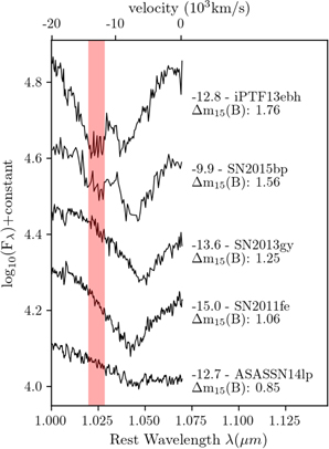
Figure 10. A zoom in on the C i 1.0693 μm feature for several well-studied SNe Ia with early NIR spectroscopy, plotted and ordered by  . Although a larger data set is necessary, a correlation between
  and C i 1.0693 μm strength is striking.
Download figure:
Standard image High-resolution image6. C ii Incidence in Transitional SNe Ia
To put our carbon observations of SN 2015bp in context we have searched the literature for nearby transitional SNe Ia with early optical spectra (any data before maximum light qualified) to gauge the incidence of carbon (C ii 6580 Å) in this subpopulation of SNe Ia. Several programs have looked at the incidence of C ii 6580 Å in early SNe Ia spectra (e.g., Parrent et al. 2011; Thomas et al. 2011; Folatelli et al. 2012; Silverman & Filippenko 2012; Maguire et al. 2014), but the transitional SNe Ia population itself has not been searched in a systematic way because of their relative rarity. While we have demonstrated the possibility that transitional SNe Ia display strong C i 1.0693 μm features in their early NIR spectra, most transitional SNe Ia do not have such data, and so we turn to the C ii 6580 Å line for our analysis for further insight. The characteristics of our collected sample are recorded in Table 7 and the early spectra (centered on C ii) are shown in Figure 11. The specific objects are largely drawn from Table 8 of Hsiao et al. (2015), with an additional object included from Ashall et al. (2019b): SN 2004eo (Pastorello et al. 2007), SN 2005am (Contreras et al. 2010; Blondin et al. 2012), SN 2007on (Folatelli et al. 2013), SN 2009an (Sahu et al. 2013), SN 2011iv (Foley et al. 2016; Gall et al. 2018), SN 2012ht (Yamanaka et al. 2014), SN 2013aj (Ashall et al. 2019b), and iPTF 13ebh (Hsiao et al. 2013).
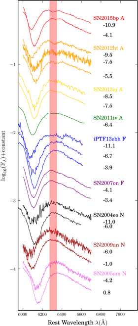
Figure 11. A zoom-in around the expected position of the C ii 6580 Å feature for our sample of nine transitional SNe Ia with early optical data. We have classified the carbon status of each SN using the scheme of Silverman & Filippenko (2012). The shaded red vertical line corresponds to an expansion velocity of 13,000 km s−1 to guide the eye toward the approximate position at which carbon may be seen.
Download figure:
Standard image High-resolution imageTable 7. Carbon Classification and Photometric Parameters of Transitional SNe Ia
| SN |

| sBV | Earliest Spec. | C ii 6580 Å |

| Si ii |
 c
c
| References, |
|---|---|---|---|---|---|---|---|---|
| (mag) | Phase (days) b | class a | (mag) | (103 km s–1) | see Notes | |||
| SN 2004eo | 1.42 ± 0.03 | 0.83 ± 0.03 | −11.0 | N | −19.08 | 10.2 | 0.093 | d |
| SN 2005am | 1.53 ± 0.02 | 0.75 ± 0.02 | −4.2 | N | −18.69 | 11.9 | 0.043 | e , f |
| SN 2007on | 1.96 ± 0.01 | 0.57 ± 0.04 | −4.1 | F | −18.24 | 11.8 | 0.001 | g |
| SN 2009an | 1.64 ± 0.04 | 0.86 ± 0.06 | −6.0 | N | −19.02 | 12.4 | 0.108 | h , m |
| SN 2011iv | 1.77 ± 0.01 | 0.64 ± 0.04 | −6.4 | A | −18.83 | 10.4 | 0.001 | i , j |
| SN 2012ht | 1.30 ± 0.04 | 0.86 ± 0.03 | −9.5 | A | −17.87 | 11.2 | 0.025 | k |
| SN 2013aj | 1.47 ± 0.01 | 0.78 ± 0.01 | −7.5 | A | −18.73 | 10.6 | 0.032 | l |
| iPTF 13ebh | 1.79 ± 0.01 | 0.63 ± 0.02 | −11.1 | F | −18.95 | 10.9 | 0.116 | m |
| SN 2015bp | 1.56 ± 0.03 | 0.671 ± 0.030 | −10.9 | A | −18.46 | 10.4 | 0.047 | This work |
Notes.
a The carbon classification scheme is adopted from Silverman et al. (2012) where “A” denotes a clear absorption feature, “F” indicates a depression or flattening of the red side of the Si ii 6355 Å, and “N” denotes spectra that do not display any carbon absorption. b The phase is with respect to the time of B-band maximum. c Total extinction applied, including Milky Way and host components. d Pastorello et al. (2007). e Contreras et al. (2010). f Blondin et al. (2012). g Folatelli et al. (2013). h Sahu et al. (2013). i Foley et al. (2016). j Gall et al. (2018). k Yamanaka et al. (2014). l Ashall et al. (2019b). m Hsiao et al. (2015).Download table as: ASCIITypeset image
For the nine transitional SNe Ia in our sample (including SN 2015bp), we display the two or three earliest available spectra in Figure 11. We adopt the carbon classification scheme of Silverman et al. (2012) (which is similar to most of the other large carbon analyses) where spectra with a distinct absorption feature associated with C ii 6580 Å are distinguished by an “A” (absorption). Spectra that show no distinct absorption feature, but a depression or a flattening of the red side of the Si ii 6355 Å feature are given an “F” (flattened); these data represent tentative carbon detections. Finally, spectra that seem to be unaffected on the red side of Si ii are denoted with an “N” (no carbon). Our carbon classifications are included in both Table 7 and Figure 11. The carbon status of several of the objects in our target sample has been remarked on elsewhere in the literature (e.g., SN 2007on, SN 2009an, SN 2012ht, and iPTF 13ebh), and in all cases our carbon assessments are in agreement. While we have not performed any spectrum synthesis modeling (e.g., SYNOW) to further bolster our carbon classifications, we believe this agreement with results in the literature verifies our visual assessment.
Four out of nine transitional SNe Ia in our sample display a clear C ii 6580 Å “notch” in our data, which we classify with an “A” (SN 2011iv, SN 2012ht, SN 2013aj, and SN 2015bp). Two further SNe have a tentative detection with a flat, or “F,” designation (SN 2007on and iPTF 13ebh). To bolster the case that a flat designation may indeed indicate a positive carbon identification, we remind the reader that iPTF 13ebh had a clear, distinct C i 1.0693 μm feature in its early NIR data. Three of our transitional SNe Ia showed no sign of carbon whatsoever (SN 2004eo, SN 2005am, and SN 2009an). The absence of carbon in SN 2004eo is notable, because a −11 days spectrum is available, although it has a relatively low signal-to-noise ratio.
The carbon statistics for our transitional SN Ia sample must be taken with caution, as previous studies have demonstrated that earlier spectra are more likely to detect C ii 6580 Å than data taken at later times, with the C ii incidence going from ∼40% at <–10 days to ∼10%–20% in the five days prior to maximum light (Parrent et al. 2011; Folatelli et al. 2012; Silverman & Filippenko 2012). The sample size of early transitional spectra is also small, prohibiting any strong conclusions. With these caveats in mind, our carbon incidence rates are broadly in line with previous work on the general SN Ia population, with ≳40% of our sample displaying a clear C ii notch. Carbon is at least as common in the transitional SNe Ia as in the general population.
With our carbon measurements of SN 2015bp and in the transitional SN Ia population in hand, we now discuss the theoretical implications of these measurements.
7. Discussion
Given the consensus that SNe Ia are the thermonuclear explosions of carbon–oxygen white dwarfs, carbon provides the most direct probe of unburned material from the progenitor white dwarf, because oxygen is also produced from carbon burning. The quantity, incidence, and distribution of unburned carbon vary between SN Ia explosion models, and so observational constraints on carbon can help distinguish between models, as we have outlined in Section 1. Here we discuss the implications of our carbon detection in SN 2015bp and the larger transitional SN Ia population.
7.1. Sub-Chandrasekhar-mass Models
Some observational studies have concluded that the faintest and fastest declining SNe Ia may result from sub-Chandrasekhar-mass ejecta (Stritzinger et al. 2006; Scalzo et al. 2014a, 2014b), and corresponding theoretical studies have also suggested that SN Ia on the faint end come from sub-Chandrasekhar-mass explosions (Blondin et al. 2017; Goldstein & Kasen 2018). If this is the case, and noting that most recent sub-Chandrasekhar models burn nearly all of the available carbon (e.g., Fink et al. 2010; Polin et al. 2019), one would expect little to no carbon in the transitional SN Ia subclass. This is in contradiction to the clear NIR C i detections in SN 2015bp and iPTF 13ebh, and the prevalence of optical C ii we see in this population (see Section 6).
To provide further context for our transitional SN Ia C ii detections, we plot their maximum light Si ii velocity versus B-band absolute magnitude in Figure 12. This plot is largely a reproduction of Figure 11 in Polin et al. (2019), with the SNe Ia sample of Zheng et al. (2018) plotted as black points in the background, as well as the transitional SNe Ia sample we introduced in Section 6.
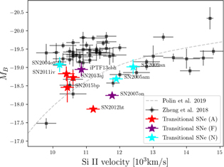
Figure 12. Plot of the peak absolute magnitude in B versus the Si ii 6355 Å velocity at the time of peak for the Zheng et al. (2018) collection of SNe Ia. We also plot the spline fit taken from the sub-Chandrasekhar double-detonation models with a thin helium shell ( ) in Polin et al. (2019). We have included our sample of transitional SNe Ia (see Table 7) with early optical spectra in this plot as well, marking those with and without optical carbon in their early data (A and N, respectively). We have also labeled those objects with a “flat” profile, which we consider a tentative C ii detection (F).
Download figure:
Standard image High-resolution imageWe tabulate the transitional SN Ia data displayed in Figure 12 in Table 7. Absolute B-band magnitudes were taken from the papers listed in the final column of the table, along with the extinction applied to reach that value; we urge the reader to look directly at these references for further details, including the distances assumed in these calculations. In most instances, we also took the peak Si ii velocity from the cited work, but when it was unavailable we retrieved the appropriate spectra and measured it ourselves using the techniques described in Section 4.1. As expected, the transitional SNe Ia sample sits at the faint and lower-velocity end of the distribution of SNe Ia. The dashed line shows a spline fit through several sub-Chandrasekhar models with a thin He shell (see Polin et al. 2019, for details) and is meant to guide the eye to show the general relationship between velocity and luminosity expected for this class of models (see also Shen et al. 2018).
As pointed out by Polin et al. (2019), two “groups” or clusters of SNe Ia are apparent in Figure 12. We note that recent work with an expanded sample indicates that these groupings may actually be part of a more continuous distribution of SN Ia properties (Burrow et al. 2020); also, no host-galaxy extinction is applied in the original presentation of Polin et al. (2019). The first grouping traces the arc of SNe Ia below the dashed line with the same general trend as the sub-Chandrasekhar models, while the second cluster forms a tight bunch with no apparent trend between silicon velocity and absolute magnitude. The SNe Ia in this second group are generally at lower velocities than those in the first group. The suggestion of Polin et al. (2019) was that these two groups represented two separate explosion mechanisms, with Chandrasekhar-mass explosions related to the tightly clumped second group, while sub-Chandrasekhar-mass explosions were responsible for the first group displaying a trend between Si ii velocity and absolute magnitude.
The transitional SNe Ia clearly have members that belong to both the “Chandrasekhar” and “sub-Chandrasekhar” subpopulations identified by Polin et al. (2019), although there is some ambiguity at the faint end of the diagram as to which population a given SN may belong. If this inference is correct, it would suggest that multiple explosion mechanisms are responsible for transitional SNe Ia since they fall within both groups. As can be seen in Figure 12, there are also clear carbon detections belonging to each population.
We conclude that at least ∼50% of transitional SNe Ia in our sample do not come from sub-Chandrasekhar-mass explosions due to the clear presence of carbon in their NIR and optical spectra. This statement is contingent on results from recent 1D sub-Chandrasekhar theoretical models, which show little to no carbon. If the amount of carbon in higher-dimension simulations increases (see, e.g., chapter 8 of Polin 2020), then this conclusion must be amended, but for now it remains an important benchmark for theoretical interpretations of the transitional SN Ia class. We next explore the possibility that our C i detections are actually misidentified He i, which may be expected in the context of double-detonation models.
7.2. Helium and Carbon Confusion in Double-detonation Models
It is possible that double-detonation models, triggered by a surface detonation of helium, will leave some unburned helium behind that would be observable in the outer ejecta. This scenario has been explored by Boyle et al. (2017), who estimated the optical depth of He i lines in the ejecta of double-detonation models, and computed synthetic spectra to track the purported helium line evolution with time. In particular, they presented calculations for the He i 1.0830 and 2.0581 μm line evolution for “high mass” (1.025 M⊙ CO core mass) and “low mass” (0.58 M⊙ CO core mass) supernova models. The high-mass model is meant to correspond to a normal-luminosity SN Ia (Fink et al. 2010), and the low-mass model was meant to represent underluminous, peculiar thermonuclear events (Sim et al. 2012). Underluminous, transitional SNe Ia such as SN 2015bp would be intermediate between these two scenarios.
In both the high-mass and low-mass models, helium absorption is visible at maximum light, and the general trend is that the helium absorption grows even stronger past maximum light (at least until +7 days, the last epoch at which they generated spectra). We do note that Boyle et al. (2017) suggest that this evolution may be somewhat model-dependent, as the helium optical depth will depend on the time evolution of the ejecta density and velocity gradient, as well as variations in the radiation temperature. The helium absorption lines are much stronger in the low-mass model where less of the helium shell gets burned, but in both instances the He i 1.0830 μm feature is prominent and roughly resembles the absorption features we identified as C i 1.0693 μm in SN 2015bp (as well as iPTF 13ebh and SN 1999by). Similar to our data, the He i 1.0830 μm absorption feature is expected to sit just blueward of Mg ii 1.0927 μm. Because of this similarity, Boyle et al. (2017) suggested that the strong C i 1.0693 μm feature identified in iPTF 13ebh and SN 1999by (and by extension, SN 2015bp) may actually be He i. However, this feature gets weaker toward maximum light in the observations of iPTF 13ebh and SN 2015bp, to the point that it becomes undetectable beyond maximum light. In contrast, the He i feature seen in the Boyle et al. (2017) simulations gets stronger (or stays at roughly the same strength) toward maximum light and continues strengthening in later phases—the opposite of the observed trend. Furthermore, both iPTF 13ebh and SN 2015bp show optical C ii 6580 Å, at least circumstantially corroborating our NIR interpretation—these SNe Ia definitively have carbon. Given this, we find the identification of this feature with He i 1.0830 μm to be unlikely, especially for the two transitional SNe Ia with strong features blueward of Mg ii. The case of the SN 1991bg–like SN 1999by may be different, because this event had a clear absorption feature blueward of Mg ii that remained strong through maximum light, and it did not display a clear optical C ii line, although the lack of early-time data precludes any definitive conclusions.
NIR spectral time-series observations of faint SNe Ia are necessary to investigate the presence of helium, and in particular K-band spectra with a high signal-to-noise ratio could enable searches for the He i 2.0581 μm line, which would be less ambiguous than the He i 1.0830 μm feature. Further modeling efforts may also be required to robustly predict the appearance and time evolution of helium in double-detonation models. Nonetheless, in transitional SNe Ia the behavior of the absorption feature blueward of Mg ii does not match current predictions for leftover helium for double-detonation SN Ia models.
7.3. Carbon in Other Scenarios
Recent analysis of several transitional SNe Ia (SN 1986G, SN 2007on, and SN 2011iv) using radiative transfer models and the abundance stratification technique have pointed to a Chandrasekhar-mass explosion consistent with delayed-detonation models (Ashall et al. 2016b, 2018), or possibly a violent merger origin (Pakmor et al. 2012) for SN 2007on due to its double-peaked nebular emission lines (Dong et al. 2015; Mazzali et al. 2018). This is in contrast to the studies mentioned earlier that point to a sub-Chandrasekhar origin for most faint SNe Ia (Blondin et al. 2017; Goldstein & Kasen 2018). If transitional SNe Ia do primarily originate from Chandrasekhar-mass delayed-detonation explosions then we would expect to see carbon in these faint events (Höflich et al. 2002), consistent with our observations. If some fraction originate from violent mergers, then leftover carbon would be expected as well (Pakmor et al. 2012). We find it more likely that one or both of these explosion mechanisms are responsible for the transitional SNe Ia subclass, given the observed incidence of carbon in our sample.
8. Summary and Conclusion
We have presented comprehensive observations of the transitional SN Ia 2015bp, the highlight of which was the early, striking detection of C i 1.0693 μm. We placed this carbon detection in context with other early NIR observations, and assessed the incidence of carbon in the transitional SN Ia population more generally. A summary of our main findings is as follows.
- 1.SN 2015bp displays all of the trademarks of the transitional SN Ia class (see, e.g., Hsiao et al. 2015). It is subluminous (
 mag) with a fast-declining light curve ( mag; ), and an NIR primary maximum that occurs before B-band maximum. No Ti ii absorption is apparent in the optical spectra. The light curve and spectroscopic parameters we measured for SN 2015bp are largely in agreement with previous work on this object (Srivastav et al. 2017).
 - 2.Early-time NIR spectra of SN 2015bp exhibit a prominent absorption line in the blue wing of Mg ii 1.0927 μm, which we attribute to C i 1.0693 μm. This feature weakens through maximum light, similar to that seen in transitional SN Ia iPTF 13ebh (Hsiao et al. 2015). The SN 1991bg–like SN 1999by, by contrast, displayed a strong C i 1.0693 μm feature past maximum light (Höflich et al. 2002).
- 3.In addition to the C i 1.0693 μm line, SN 2015bp also displays a clear C ii 6580 Å notch at early times. The velocities of the C i and C ii features are consistent with each other to within ∼1000 km s−1, and are marginally above the photosphere as measured by the Si ii 6355 Å absorption line velocity.
- 4.There appears to be a correlation between the strength of the C i 1.0693 μm absorption feature and the light-curve decline rate in SNe Ia with NIR data at very early times (≲−10 days; see Figure 10) in the sense that faster declining events have more apparent carbon (see also Hoeflich et al. 2017; Hsiao et al. 2019). Of note, it is only in fast-declining SNe Ia that the C i 1.0693 μm feature is conspicuous in the blue wing of Mg ii. Further data of a variety of SNe Ia at early times are needed to verify this and to confirm the trend mentioned above.
- 5.Given the presence of strong NIR C i in the early-time spectra of both SN 2015bp and iPTF 13ebh, we investigated the incidence of early optical C ii 6580 Å in a larger sample of transitional SNe Ia. Four out of nine transitional SNe Ia in our sample display a clear C ii notch, while two others have tentative “flat” detections. With the caveat that we are in the small-numbers regime, our carbon incidence rate is broadly in line with previous work on the general SN Ia population, and stands at ≳40%.
- 6.We find it unlikely that the NIR C i feature is actually misidentified He i, as suggested for double-detonation models (Boyle et al. 2017). The observed C i feature seen in SN 2015bp and iPTF 13ebh weakens up through maximum light, while the He i predicted by the double-detonation models strengthens over the same time period. The clear presence of optical C ii in SN 2015bp further bolsters the case that the strong NIR absorption feature is C i.
- 7.The presence of strong NIR carbon in SN 2015bp and iPTF 13ebh, along with the incidence of optical carbon in the transitional SNe Ia class, argues against a sub-Chandrasekhar origin for these faint SNe Ia despite recent modeling efforts (Blondin et al. 2017; Goldstein & Kasen 2018). Carbon in the transitional SNe Ia is consistent with originating from Chandrasekhar-mass delayed-detonation and/or violent merger explosions, as other work has suggested (e.g., Ashall et al. 2016b, 2018).


Several avenues of future research present themselves; while we focus on work associated with the detection of carbon here, other areas such as nebular spectroscopy of comprehensive samples of faint type Ia SNe may also prove fruitful. First, very early-time NIR spectroscopic sequences of Type Ia SNe are still rare, but it is clear that more data sets are necessary to solidify tentative correlations between NIR C i strength and light-curve decline rate, as suggested by Figure 10. Extending these early-time observations to include K-band observations with high signal-to-noise ratio would allow useful searches for helium, a prediction of double-detonation models. Furthermore, larger samples of early-time optical spectra may identify the incidence of carbon among subpopulations of Type Ia SNe (i.e., as a function of position on the iconic Branch diagram or the “Polin plot” as seen in Figure 12) and would go hand in hand with modeling efforts as the community tries to understand the viable explosion mechanisms for SNe Ia. Indeed, a couple of recent, faint type I supernovae—SN 2018byg (De et al. 2019) and SN 2016jhr (Jiang et al. 2017)—do have the hallmarks of a sub-Chandrasekhar double-detonation explosion, showing that this explosion model is viable, at least for peculiar SNe. This comprehensive study of SN 2015bp and the transitional SNe Ia population in general show the continued promise of unburned carbon for testing explosion models.
We thank D. K. Sahu for providing early-time optical spectra of SN 2009an.
Research by D.J.S. is supported by NSF grants AST-1821967, AST-1821987, AST-1813708, AST-1813466, and AST-1908972, as well as by the Heising-Simons Foundation under grant #2020-1864. The CSP-II has been supported by National Science Foundation (NSF) grants AST-1008343, AST-1613426, AST-1613455, and AST-1613472, as well as by the Danish Agency for Science and Technology and Innovation through a Sapere Aude Level 2 grant. E.Y.H. and J.L. also acknowledge the support of the Florida Space Grant Consortium. This work was partially performed at the Aspen Center for Physics, which is supported by NSF grant PHY-1607611. Research by S.V. is supported by NSF grants AST1813176 and AST-2008108. L.G. was funded by the European Union’s Horizon 2020 research and innovation program under the Marie Skłodowska-Curie grant agreement No. 839090. This work has been partially supported by the Spanish grant PGC2018-095317-B-C21 within the European Funds for Regional Development (FEDER). M.S. is supported by generous grants from Villum FONDEN (13261, 28021) and by a project grant (8021-00170B) from the Independent Research Fund Denmark. A.V.F. is grateful for financial assistance from the TABASGO Foundation, the Christopher R. Redlich Fund, and the Miller Institute for Basic Research in Science (U.C. Berkeley).
Based on observations obtained at the international Gemini Observatory (GN-2015A-Q-8, GS-2015A-Q-5), a program of NSF’s NOIRLab, which is managed by the Association of Universities for Research in Astronomy (AURA) under a cooperative agreement with the National Science Foundation. on behalf of the Gemini Observatory partnership: the National Science Foundation (United States), National Research Council (Canada), Agencia Nacional de Investigación y Desarrollo (Chile), Ministerio de Ciencia, Tecnología e Innovación (Argentina), Ministério da Ciência, Tecnologia, Inovações e Comunicações (Brazil), and Korea Astronomy and Space Science Institute (Republic of Korea). This paper includes data gathered with the Nordic Optical Telescope (PI Stritzinger) at the Observatorio del Roque de los Muchachos, La Palma, Spain.
This work is based in part on observations from the Deep Imaging Multi-Object Spectrograph at the Keck II telescope. We are grateful to the staff at the Keck Observatory for their assistance, and we extend special thanks to those of Hawaiian ancestry on whose sacred mountain we are privileged to be guests. The W. M. Keck Observatory is operated as a scientific partnership among the California Institute of Technology, the University of California, and NASA; it was made possible by the generous financial support of the W. M. Keck Foundation. We thank S. Bradley Cenko for assistance with the Keck spectral reductions, as well as Patrick Kelly, WeiKang Zheng, and John Mauerhan for their assistance with the observations.
D.J.S. is a visiting Astronomer at the Infrared Telescope Facility, which is operated by the University of Hawaii under contract 80HQTR19D0030 with the National Aeronautics and Space Administration. Based on data products from observations made with ESO Telescopes at the La Silla Paranal Observatory under programmes 188.D-3003 and 191.D-0935: PESSTO (the Public ESO Spectroscopic Survey for Transient Objects).
Facilities: Swope - Swope Telescope, Du Pont (Retrocam) - , NTT (EFOSC2 - , SOFI) - , NOT (ALFOSC) - , Gemini:Gillett (GNIRS) - , Gemini:South (F2) - , IRTF (SpeX) - , Magellan:Baade (FIRE) - .
Software: Astropy (Astropy Collaboration et al. 2018), IDL (Landsman 1993), Matplotlib (Hunter 2007), NumPy (Walt et al. 2011), SNooPy (Burns et al. 2011).
Footnotes
- *
This paper includes data gathered with the 6.5 m Magellan Telescope at Las Campanas Observatory, Chile.
- 16
These spectra were collected from the Open Supernova Catalog (Guillochon et al. 2017): https://sne.space/.