Abstract
In this work, we propose new statistical tools that are capable of characterizing the simultaneous dependence of dark matter and gas clustering on the scale and the density environment, and these are the environment-dependent wavelet power spectrum (env-WPS), the environment-dependent bias function (env-bias), and the environment-dependent wavelet cross-correlation function (env-WCC). These statistics are applied to the dark matter and baryonic gas density fields of the TNG100-1 simulation at redshifts of z=3.0-0.0, and to Illustris-1 and SIMBA at z = 0. The measurements of the env-WPSs suggest that the clustering strengths of both the dark matter and the gas increase with increasing density, while that of a Gaussian field shows no density dependence. By measuring the env-bias and env-WCC, we find that they vary significantly with the environment, scale, and redshift. A noteworthy feature is that at z = 0.0, the gas is less biased in denser environments of Δ ≳ 10 around 3 h Mpc−1, due to the gas reaccretion caused by the decreased AGN feedback strength at lower redshifts. We also find that the gas correlates more tightly with the dark matter in both the most dense and underdense environments than in other environments at all epochs. Even at z = 0, the env-WCC is greater than 0.9 in Δ ≳ 200 and Δ ≲ 0.1 at scales of k ≲ 10 h Mpc−1. In summary, our results support the local density environment having a non-negligible impact on the deviations between dark matter and gas distributions up to large scales.
Original content from this work may be used under the terms of the Creative Commons Attribution 4.0 licence. Any further distribution of this work must maintain attribution to the author(s) and the title of the work, journal citation and DOI.
1. Introduction
In the standard paradigm of galaxy formation, small density fluctuations of baryonic gas start to grow and develop together with those of dark matter under the gravitational instability following recombination. At later times, dark matter fluctuations, once they exceed some threshold, will collapse into virialized halos, within which partial gas condenses and cools to form galaxies (Mo et al. 2010). Therefore, galaxies are biased discrete tracers of the underlying matter distribution, while the gas, as the continuously fluctuating medium, may better trace the matter distribution. On the simulation side, many studies have confirmed that the baryonic gas follows the underlying dark matter distribution on large scales quite well. For example, the power spectrum of the gas density field is very close to that of dark matter (e.g., Cui & Zhang 2017; Springel et al. 2018), the spatial distributions of the dark matter and the baryonic gas are highly correlated with each other over a wide range of scales (e.g., Yang et al. 2020, 2021), and the gas alone can be used to classify the cosmic web in an unbiased manner (e.g., Cui et al. 2018). Additionally, the intergalactic gas distribution is receiving increasing attention in observations. Measuring the large-scale structures of the universe traced by gas is the goal of a number of upcoming surveys, such as the Canadian Hydrogen Intensity Mapping Experiment (CHIME; Bandura et al. 2014), the Hydrogen Intensity and Real-time Analysis eXperiment (HIRAX; Newburgh et al. 2016), and the Square Kilometre Array (SKA; Bacon et al.2020).
As the scale becomes smaller, galaxy formation processes, such as gas cooling, star formation, and feedbacks, have an increasing influence on the matter clustering, thereby resulting in a significant bias between the gas and the dark matter. In particular, the clustering of the gas is strongly suppressed up to scales a few times 0.1 h Mpc−1, mainly due to the active galactic nuclei (AGN) feedback, which heats and ejects gas from halos (van Daalen et al. 2019), while the star formation consumes the available gas on galactic scales. Due to the combined effects of nonlinear gravitational evolution and complex baryonic physical processes, the matter distribution becomes highly non-Gaussian at small scales and low redshifts. Moreover, it is well known that there is a strong relationship between a galaxy’s properties and its density environments. For instance, massive and quenched galaxies tend to occur in high-density environments (e.g., Hoyle et al. 2012; Moorman et al. 2016), and the star formation rates of galaxies increase with environmental density at redshifts z ≳ 1, but decrease with environmental density at redshifts z ≲ 1 (e.g., Cooper et al. 2008; Wang et al. 2018; Hwang et al. 2019). The environmental dependence of galactic properties may imply two aspects. First, galaxies in high-density environments interact more frequently and therefore strip their gas faster than those in low-density environments. Second, feedback (e.g., AGN feedback) efficiency varies in different density environments. For example, Miraghaei (2020) found in Sloan Digital Sky Survey Data Release 7 that underdense regions have a higher fraction of thermal-mode AGNs than overdense regions, for massive red galaxies, whereas kinetic-mode AGNs prefer to reside in denser regions.
According to the above statements, deviations of the spatial clustering between the gas and the dark matter are expected to depend on both the scale and the density environment. Quantifying such simultaneous dependence on the scale and the environment will hopefully deepen our understanding of the extent to which baryonic gas follows dark matter. To achieve this goal, statistical tools that can give the frequency information, while retaining the spatial information, are required. However, the traditional two-point correlation function or its Fourier counterpart, the power spectrum, is only a univariate function of scale and totally insensitive to non-Gaussianity, so it is not up to the task. A variety of advanced statistics beyond the power spectrum have been previously developed, including but not limited to the bispectrum, which is a third-order spectrum (see, e.g., Sefusatti et al. 2006; Foreman et al. 2020), the position-dependent power spectrum, based on the windowed Fourier transform (Chiang et al. 2014), the sliced correlation function (Neyrinck et al. 2018), and the k-nearest neighbor cumulative distribution functions (Banerjee & Abel 2020). Since the processes associated with galaxy formation are very complex and poorly understood, predictions from different statistics are vital to improving our knowledge of galaxy formation.
As a bivariate function of scale and space, wavelet transforms are particularly suitable for the issue we are interested in. With a basis function (i.e., a “wavelet”) that is well localized, both in the real domain and the frequency domain, the wavelet transform acts like a “mathematical microscope,” which allows us to zoom in on fine structures of the universe at various scales and locations (e.g., Kaiser & Hudgins 1994; Addison 2017). There are two major types of wavelet transforms—the discrete wavelet transform (DWT) and the continuous wavelet transform (CWT)—both of which are widely employed in cosmology (see, e.g., Martínez et al. 1993; Pando & Fang 1996; Fang & Feng 2000; Starck et al. 2004; Liu & Fang 2008; Zhang et al. 2011; Arnalte-Mur et al. 2012; da Cunha et al. 2018; Shi et al. 2018; Copi et al. 2019; Wang et al. 2021). Besides, there are also some other wavelet transform variants, e.g., the wavelet scattering transform (Mallat 2012), which performs two operations repeatedly—(1) wavelet convolution and (2) modulus—and has been proved to be superior to the Fourier power spectrum for cosmological parameter inference (e.g., Allys et al. 2020; Cheng et al. 2020; Valogiannis & Dvorkin 2022). However, using wavelets to investigate the scale and environmental dependence of matter clustering seems to have been neglected in most previous studies. Due to the arbitrary scale choices and translational invariance of the CWT (Addison 2017), we will employ it to analyze the deviation between the dark matter and gas distributions, and quantify its dependence on both the scale and density environment.
The most criticized aspect of the CWT is that its computation consumes more time and resources than that of the DWT. However, the Fourier convolution theorem allows us to compute the CWT quickly, by utilizing a fast Fourier transform (FFT) with a complexity of  at each scale (Torrence & Compo 1998). In addition to this, much research has been dedicated to the fast implementation of the CWT in the real domain (Rioul 1991; Unser et al. 1994; Berkner & Wells 1997; Vrhel et al. 1997; Muñoz et al. 2002; Omachi & Omachi 2007; Patil & Abel 2009; Arizumi & Aksenova 2019). For example, by decomposing the wavelet function and signal into B-spline bases, Muñoz et al. (2002) converted the CWT into a convolution of two B-splines, which could be expressed analytically and had a lower number of operations. Omachi & Omachi (2007) achieved a fast computation of the CWT by representing the wavelet as a polynomial within its compact support interval. The most recent algorithm, proposed by Arizumi & Aksenova (2019), approximates the mother wavelet as piecewise polynomials. Although it is claimed that all these algorithms are better than FFT, they are restricted to 1D and special wavelets. Therefore, the efficiency of these methods might not be guaranteed for general wavelet functions or for high dimensions. In the present work, the fast computation of CWT is implemented by the FFT.
In a previous work (Wang & He 2021), we developed a new method for designing continuous wavelets, in which those wavelets are constructed by taking the first derivative of the smoothing function, e.g., the Gaussian function, with respect to the positively defined scale parameter. The convenience of this method is due to the original signal being reconstructed through a single integral of the continuous wavelet coefficients. Furthermore, Wang et al. (2021) introduced wavelet-based statistical quantities, including the wavelet power spectrum (WPS), wavelet cross-correlation (WCC), and wavelet bicoherence. By evenly splitting the whole simulation box into subcubes, Wang et al. (2021) suggest that the properties of the matter clustering depend on the local mean density of the subcube. However, we realize that this is not a wise way to divide the environment and that it does not fully reflect the power of the wavelet techniques. On the one hand, the cubic environment could not isolate a special structure, say a halo, from its surroundings. On the other hand, the CWT varies with the spatial position at a fixed scale, and therefore with the local density at that location. Following this idea, we can build more flexible wavelet statistics that depend directly on the local density and scale. In this study, we propose the environment-dependent wavelet power spectrum (env-WPS) and the environment-dependent wavelet cross-correlation function (env-WCC). The env-WPS measures the strength of the matter clustering across different scales within a density interval, while the env-WCC measures the statistical coherence of the spatial distributions between the gas and the dark matter. The environment-dependent bias function (env-bias) reflects the scale- and environment-dependent bias between the gas and the dark matter.
The environmental dependence requires wavelets with good spatial resolution, and the scale dependence requires wavelets with good frequency resolution. As a result, a wavelet that can achieve a good trade-off between these two resolutions is necessary. To achieve this, the analytic wavelet function that we use here is derived from a Gaussian function weighted by a cosine function, which has a better frequency resolution than the Gaussian-derived wavelet (GDW) used in previous works (Wang & He 2021; Wang et al. 2021) and also maintains a reasonable spatial resolution. In this study, we apply the env-WPS and the env-WCC to the density fields of three cosmological simulations: Illustris (Nelson et al. 2015), IllustrisTNG (Nelson et al. 2019), and SIMBA (Davé et al. 2019).
The rest of this work is structured as follows. We briefly describe the simulations we used in Section 2, and introduce the fundamental theories in Section 3. Our main results regarding the dependence of the matter clustering on both the scale and the environment are given in Section 4. Finally, in Section 5, we discuss and summarize our main findings and present the conclusions.
For convenience of the readers, in Table 1, we list the wavelet-related acronyms used in our paper, with their meanings.
Table 1. The Wavelet-related Acronyms Used in the Paper, with Their Meanings Explained
| Acronym | Meaning |
|---|---|
| CWT | continuous wavelet transform |
| GDW | Gaussian-derived wavelet |
| CW-GDW | cosine-weighted Gaussian-derived wavelet |
| WPS | wavelet power spectrum |
| WCC | wavelet cross-correlation |
| env-WPS | environment-dependent wavelet power spectrum |
| env-WCC | environment-dependent wavelet cross-correlation function |
| env-bias | environment-dependent bias function |
Download table as: ASCIITypeset image
2. Data Sets
For our analysis, we utilize three state-of-the-art cosmological simulations: Illustris 3 (Vogelsberger et al. 2013, 2014; Genel et al. 2014; Nelson et al. 2015), IllustrisTNG 4 (Marinacci et al. 2018; Naiman et al. 2018; Nelson et al. 2018, 2019; Pillepich et al. 2018a; Springel et al. 2018), and SIMBA 5 (Davé et al. 2019). In particular, we mainly focus on the density fields drawn from the IllustrisTNG100-1 run at redshifts z = 0, 1, 2, and 3. The present-day (z = 0) density fields of the Illustris-1 and fiducial SIMBA run (m100n1024) are used for comparison to that of IllustrisTNG100-1.
- 1.The Illustris simulation tracks the evolution of the baryonic and dark matter from redshift z = 127 to the present day, by using the adaptive moving-mesh AREPO code (Springel 2010). The adopted cosmological parameters are ΩΛ = 0.7274, Ωm = Ωdm + Ωb = 0.2726, Ωb = 0.0456, σ8 = 0.809, ns = 0.9631, and h = 0.704, consistent with the constraints from WMAP-9 (Bennett et al. 2013). The subgrid models of galaxy formation are described in detail in Vogelsberger et al. (2013) and Torrey et al. (2014), including star formation and associated supernova feedback, supermassive black hole accretion, and related AGN feedback (thermal-mode and kinetic-mode). In fact, the AGN feedback in Illustris is so effective that it can lead to a lower gas fraction in the halos, which is in conflict with the observations (Genel et al. 2014). The Illustris-1 run that we used has a box of volume
 and contains 18203 dark matter particles of mass ∼6.26 ×10⁶
M⊙, plus 18203 initial gas cells with average mass ∼1.26 × 10⁶
M⊙.
and contains 18203 dark matter particles of mass ∼6.26 ×10⁶
M⊙, plus 18203 initial gas cells with average mass ∼1.26 × 10⁶
M⊙. - 2.The IllustrisTNG (hereafter, TNG) simulation is the successor of the Illustris project, which is also executed with the AREPO code and consists of three simulation volumes: TNG300, TNG100, and TNG50. All these runs assume Planck concordance cosmology (Planck Collaboration XIII 2016), i.e., ΩΛ = 0.6911, Ωm = Ωdm +Ωb = 0.3089, Ωb = 0.0486, σ8 = 0.8159, ns = 0.9667, and h = 0.6774. Compared with earlier Illustris simulations, TNG uses updated physical models and numerical methods and yields better consistency with the available observations of galaxy formation and evolution. Thus, it provides us with an ideal laboratory for testing theoretical models and developing new analysis tools to achieve a more precise understanding of structure formation and galaxy formation. The details of the TNG model for galaxy formation are given in Pillepich et al. (2018b) and Weinberger et al. (2018). In this work, we use density fields of the TNG100-1 simulation at redshifts z = 0.0, 1.0, 2.0, and 3.0. This simulation adopts a periodic box of side length Lbox = 75 h−1 Mpc ≃ 110.7 Mpc, and uses the same initial conditions as Illustris-1. The mass of each dark matter particle is ∼7.5 × 10⁶ M⊙ and the initial baryonic mass resolution is ∼1.4 × 10⁶ M⊙.
- 3.The SIMBA simulation suite is performed with the meshless finite-mass hydrodynamics code GIZMO (Hopkins 2015), and includes four simulation volumes: m100n1024, m50n1024, m25n1024, and m12.5n1024, all starting at z = 249 and ending at z = 0. These simulations also assume the Planck concordance cosmology (Planck Collaboration XIII 2016): ΩΛ = 0.7, Ωm = Ωdm + Ωb = 0.3, Ωb = 0.048, σ8 = 0.82, ns = 0.97, and h = 0.68. The implementation of the galaxy formation physics in this simulation, e.g., AGN feedback, stellar feedback, gas cooling, and star formation, can be found in Davé et al. (2019). With these sophisticated models, SIMBA is also capable of reproducing a wide range of observations. The fiducial SIMBA run (m100n1024) used here has a box size of 100 h−1 Mpc ≃ 147 Mpc, with 10243 dark matter particles plus 10243 gas cells. The mass resolution is ∼ 9.6 ×10⁷ M⊙ for dark matter and ∼ 1.82 × 10⁷ M⊙ for gas.

3. Continuous Wavelet Methods
3.1. The 1D Cosine-weighted Gaussian-derived Wavelet
In previous works (Wang & He 2021; Wang et al. 2021), we applied the GDW, a low-oscillation wavelet, to the spectral analysis of the matter clustering in 1D and isotropic cases. However, low-oscillation wavelets are more extended in Fourier space, which can mean that the results of spectral analysis at small scales are contaminated by large scales (Frick et al. 2001). To achieve a better separation of scales, we take the Gaussian function weighted by the cosine as the smoothing function, then derive the wavelet from it. In 1D, the form of such a cosine-weighted Gaussian-derived wavelet (CW-GDW) is constructed as below. From the cosine-weighted Gaussian smoothing function
with its Fourier transform
we have the CW-GDW
and its Fourier transform
where the dimensionless constant α ≃ 2.20473, which is used to set w to be the peak frequency of  . The index κ = 1/2 guarantees that the integral of the square of the wavelet is conserved across different scales. Compared to the GDW, the CW-GDW has better spectral resolution, as shown in Figure 1. This wavelet can be generalized to higher dimensions, for analyzing the large-scale structures of the universe. The isotropic and anisotropic CW-GDWs are both described as follows.
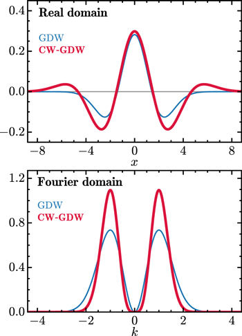
Figure 1. Comparison of the 1D GDW (thin line) and CW-GDW (thick line) in the real (top) and Fourier (bottom) domain, at scale w = 1. For presentational convenience, all variables are dimensionless.
Download figure:
Standard image High-resolution image3.2. The 3D Isotropic CW-GDW Transform
The 3D isotropic CW-GDW is defined in Fourier space by taking the derivative of the isotropic cosine-weighted Gaussian smoothing function  w.r.t. w,
with
where the index κ = −1/2, in this case. It can be seen that  depends only on the magnitude of the wavevector, i.e.,
  , which is shown in the lower panel of Figure 2. The isotropic CW-GDW Ψ(w,
r
) in real space can be computed numerically by FFT, which is plotted in the upper panel of Figure 2.
, which is shown in the lower panel of Figure 2. The isotropic CW-GDW Ψ(w,
r
) in real space can be computed numerically by FFT, which is plotted in the upper panel of Figure 2.
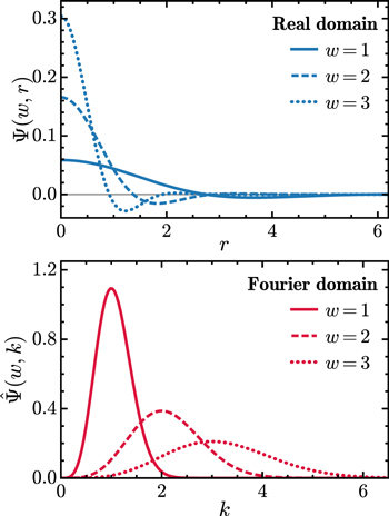
Figure 2. The isotropic CW-GDW in the real (top) and Fourier (bottom) domain, at three scales, w = 1, 2, and 3. For presentational convenience, all variables are dimensionless.
Download figure:
Standard image High-resolution imageBy convolving the density contrast  with the isotropic CW-GDW, we get the wavelet transform
where  is the Fourier transform of δ(
r
), which is estimated by interpolating the mass of each particle to a regular grid with 10243 cells, using the cloud-in-cell method. From Equation (4), the CWT corresponds to a local filtering of δ(
r
) around wavenumber ∣
k
∣ ∼ w. According to Appendix B of Wang et al. (2021), the original density field can be reconstructed by
is the Fourier transform of δ(
r
), which is estimated by interpolating the mass of each particle to a regular grid with 10243 cells, using the cloud-in-cell method. From Equation (4), the CWT corresponds to a local filtering of δ(
r
) around wavenumber ∣
k
∣ ∼ w. According to Appendix B of Wang et al. (2021), the original density field can be reconstructed by

In many investigations, the comparison between a wavelet transform and a Fourier transform at a given scale requires the correspondence between the wavelet scale w and the Fourier wavenumber ∣ k ∣, which is

with cw ≃ 0.85617 for the isotropic CW-GDW, determined by the wavelet spectral peak of a harmonic wave with frequency ∣ k ∣ (e.g., Meyers et al. 1993; Torrence & Compo 1998; Wang et al. 2021).
3.3. The 3D Anisotropic CW-GDW Transform
Following the logic of Wang & He (2021), the 3D anisotropic CW-GDW can be obtained from the 1D version, as shown below:
with the Fourier transform

where the index κ = 1/2,  is the anisotropic cosine-weighted Gaussian smoothing function with
r
= (x, y, z), and
w
= (wx
, wy
, wz
) is the scale vector. In contrast to the isotropic CW-GDW, which can only dilate or contract in the radial direction, the anisotropic one can have different dilations along different spatial axes. For example, three scale configurations—
w
= (1, 1, 1), (1, 2, 1), and (1, 2, 2)—are illustrated in Figure 3. Intuitively, the CW-GDW with a scale of (1, 1, 1) may have a stronger response to the clumps of the cosmic web, while those with scales of (1, 2, 1) and (1, 2, 2) may have better responses to the sheet and filamentary structures, respectively.
is the anisotropic cosine-weighted Gaussian smoothing function with
r
= (x, y, z), and
w
= (wx
, wy
, wz
) is the scale vector. In contrast to the isotropic CW-GDW, which can only dilate or contract in the radial direction, the anisotropic one can have different dilations along different spatial axes. For example, three scale configurations—
w
= (1, 1, 1), (1, 2, 1), and (1, 2, 2)—are illustrated in Figure 3. Intuitively, the CW-GDW with a scale of (1, 1, 1) may have a stronger response to the clumps of the cosmic web, while those with scales of (1, 2, 1) and (1, 2, 2) may have better responses to the sheet and filamentary structures, respectively.
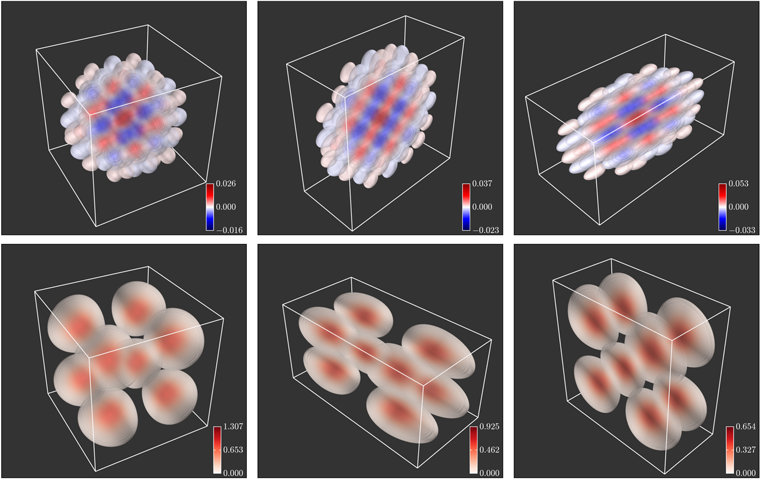
Figure 3. Contour plots of the anisotropic CW-GDW with different scales, in real space (upper panels) and in Fourier space (lower panels). Left column: the anisotropic CW-GDW and its Fourier counterpart at scale w = (1, 1, 1). Middle column: the anisotropic CW-GDW and its Fourier counterpart at scale w = (1, 2, 1). Right column: the anisotropic CW-GDW and its Fourier counterpart at scale w = (1, 2, 2).
Download figure:
Standard image High-resolution imageBy using the anisotropic CW-GDW, the wavelet transform of the density contrast δ( r ) is given by
In this anisotropic case, the reconstruction formula is a triple integral w.r.t. the scale space,
which is the extension of the 1D reconstruction formula given in Wang et al. (2021). The relation between the wavelet scale w = (wx , wy , wz ) and the Fourier wavevector k = (kx , ky , kz ) is

with cw ≃ 0.94411, determined by the wavelet spectral peak of a harmonic wave in each spatial axis.
3.4. Wavelet Statistics
Being the inverse Fourier transforms of  or
or  , the CWTs of density fields can be efficiently implemented by FFT. For illustration, we compare in Figure 4 the CWTs of the TNG100-1 dark matter density field δdm(
r
) at z = 0 and the Gaussian field constructed by randomizing phases of
, the CWTs of density fields can be efficiently implemented by FFT. For illustration, we compare in Figure 4 the CWTs of the TNG100-1 dark matter density field δdm(
r
) at z = 0 and the Gaussian field constructed by randomizing phases of  . Therefore, these two fields share the same power spectrum, which is totally insensitive to non-Gaussianity. In contrast, the CWT of the non-Gaussian dark matter field is completely different from that of the Gaussian field, which is attributed to the CWT preserving both the scale information and the spatial texture of the fields. Notice that clusters are highlighted by the isotropic CW-GDW and anisotropic CW-GDW, with a scale of
w
= (4.09, 4.09, 4.09) h Mpc−1, and the vertical and horizontal filaments are captured by the anisotropic CW-GDWs with
w
= (5, 0.5, 5) h Mpc−1 and
w
= (0.5, 5, 5) h Mpc−1, respectively. Because the CWT of the density field varies with the spatial coordinate
r
at a given scale, it should be a function of the local density fluctuation δ(
r
). With this in mind, we can interpret the simultaneous dependence of the matter clustering on the scale and the density environment using statistics developed from the CWT.
. Therefore, these two fields share the same power spectrum, which is totally insensitive to non-Gaussianity. In contrast, the CWT of the non-Gaussian dark matter field is completely different from that of the Gaussian field, which is attributed to the CWT preserving both the scale information and the spatial texture of the fields. Notice that clusters are highlighted by the isotropic CW-GDW and anisotropic CW-GDW, with a scale of
w
= (4.09, 4.09, 4.09) h Mpc−1, and the vertical and horizontal filaments are captured by the anisotropic CW-GDWs with
w
= (5, 0.5, 5) h Mpc−1 and
w
= (0.5, 5, 5) h Mpc−1, respectively. Because the CWT of the density field varies with the spatial coordinate
r
at a given scale, it should be a function of the local density fluctuation δ(
r
). With this in mind, we can interpret the simultaneous dependence of the matter clustering on the scale and the density environment using statistics developed from the CWT.
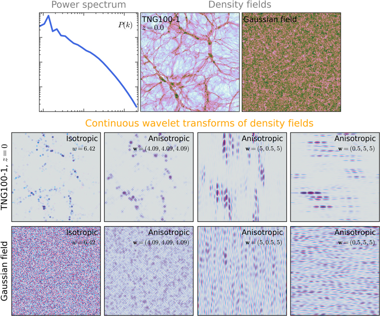
Figure 4. Top row: the TNG100-1 dark matter density field at z = 0 and the Gaussian field with the same Fourier power spectrum in a 75 × 75 h−2 Mpc2 slice of thickness 1 h−1 Mpc. Middle row: the CWTs of the TNG100-1 field in the same slice. Specifically, the left plot is the isotropic CW-GDW transform at scale w = 6.42 h Mpc−1. The three plots on the right are anisotropic CW-GDW transforms at scales of w = (4.09, 4.09, 4.09) h Mpc−1, (5, 0.5, 5) h Mpc−1, and (0.5, 5, 5) h Mpc−1, respectively. Bottom row: the same as the middle row, but for the Gaussian field with the equivalent power spectrum. By using Equations (6) and (11), it can be seen that all these wavelet scales correspond to a Fourier scale of ∣ k ∣ ≈ 7.5 h Mpc−1.
Download figure:
Standard image High-resolution imageWe now introduce some wavelet statistics by means of the isotropic CW-GDW transform. To measure the clustering strength in different environments, we take the average of the wavelet coefficients at each scale with the same local density, i.e., δ( r ) = δ, which is designated as the env-WPS, as shown below:

where the subscript “i” refers to either dark matter or gas, and Wi(w,
r
) is the isotropic CW-GDW transform of the corresponding density field. We use  to denote the density field of the total matter, with δ(
r
) = (Ωdm
δdm(
r
) + Ωb
δgas(
r
))/Ωm.
6
Practically, the densities are divided into 16 bins: (a) 14 logarithmic bins equally divided between Δ = 0.1 and Δ = 200; (b) one with Δ < 0.1 (extreme underdense environments); and (c) one with Δ > 200 (usually the halo environments). If we average over all the possible densities, then the env-WPS will degenerate to the global WPS,
to denote the density field of the total matter, with δ(
r
) = (Ωdm
δdm(
r
) + Ωb
δgas(
r
))/Ωm.
6
Practically, the densities are divided into 16 bins: (a) 14 logarithmic bins equally divided between Δ = 0.1 and Δ = 200; (b) one with Δ < 0.1 (extreme underdense environments); and (c) one with Δ > 200 (usually the halo environments). If we average over all the possible densities, then the env-WPS will degenerate to the global WPS,

which is proportional to the Fourier power spectrum (Wang et al. 2021).
We define the env-bias as the square root of the ratio of the env-WPS of gas to that of dark matter,
which enables the dark matter CWT to be reconstructed from the gas CWT, as illustrated below:

where the gas CWT Wgas(w, r ) is divided by the env-bias bW (w, δ), if δ( r ) is in the density bin δ. Inspired by the bias research (Bonoli 2009) based on the Fourier power spectrum, the reconstruction error can be estimated by
According to Equations (12) and (13), we arrive at
where CW (w, δ) is defined as
namely, the env-WCC between the gas and dark matter fields. It is a measure of the statistical coherence between these two fields, and takes values between −1 and 1. If CW (w, δ) = 1, then the fields are totally correlated, hence the dark matter can be fully determined from the gas by bW (w, δ). On the other hand, if CW (w, δ) = − 1, then the fields are totally anticorrelated. Apparently, once bW (w, δ) and CW (w, δ) are known, the characteristics of the dark matter field can be constrained more accurately from the baryonic observations.
Notice that the above statistics are built on the assumption of an isotropic matter distribution. Generally, the anisotropic statistics as functions of the scale vector w and the local overdensity δ can be derived from the anisotropic CW-GDW transform in the same way. For instance, the anisotropic env-WPS, env-bias, and env-WCC are

respectively. By taking the average of these anisotropic statistics over all w with the same modulus, they will reduce to the isotropic ones defined by Equations (12), (13), and (14), i.e.:
Since we only care about the dependence of the clustering on the scale modulus w and the local density δ, and also for the sake of minimizing computational effort, we will use those statistics based on the isotropic CW-GDW. 7
4. Results
We present our main results for the dark matter and baryonic gas clustering at redshifts 0 ≤ z ≤ 3. In particular, we explore how the dark matter and gas clustering depends on the environment by computing the env-WPS. We also quantify the deviation between the dark matter and gas distributions by computing the env-bias and env-WCC. In all the results below, the wavelet scale w is expressed as the Fourier wavenumber k, according to the relation given by Equation (6). To ensure that our results are unaffected by aliasing effects, we only consider the scales of w < cw kNyq/2, where kNyq = 1024π/Lbox is the Nyquist frequency.
4.1. The Env-WPS of the Density Field
In Figure 5, we compare the env-WPSs of a statistically homogeneous Gaussian random field with power-law spectrum P(k) ∝ k−2 and the TNG100-1 dark matter density field at redshift z = 0. For the Gaussian field, which is completely characterized by the Fourier power spectrum, we can see that its env-WPS shows no environmental dependence. However, for the dark matter field at z = 0, the env-WPS exhibits a strong dependence on the density environment, confirming that this field is highly non-Gaussian. We show the evolution of the environmental dependence of the matter clustering with redshift in Figure 6, in which we focus on the env-WPSs of the dark matter and gas at z = 3.0, 2.0, 1.0, and 0.0. Now let us consider the behavior of the dark matter. At z = 3, WPSs in different environments already exhibit different clustering strengths, except on the largest scales, where they all converge to the global WPS. Specifically, the env-WPS monotonically increases toward higher-density environments on almost all scales. This result is intuitive, because high-density environments contain more gravitationally bound objects (e.g., halos and subhalos) than low-density environments (e.g., Maulbetsch et al. 2007). At lower redshifts, the env-WPS continues to maintain the same dependence on density environment with enhanced amplitude, mainly due to nonlinear gravitational effects. For the gas component, its env-WPS follows the behaviors of the dark matter. However, on intermediate and small scales, the env-WPSs of the gas are suppressed, due to baryonic processes resisting the collapse of gas, particularly due to AGN feedback, which heats and expels gas from halos to large radii (e.g., van Daalen et al. 2019).
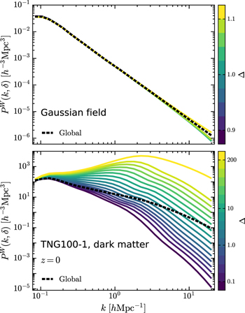
Figure 5. Comparison of the env-WPS of the Gaussian density field and that of the non-Gaussian density field. Top panel: the env-WPS of the Gaussian density field with power-law power spectrum P(k) ∝ k−2. Bottom panel: the env-WPS of the TNG100-1 dark matter density field at z = 0, which is highly non-Gaussian. The environment is defined according to the density division scheme described in Section 3.4, in descending order of density from top to bottom. The global WPS is plotted as a dashed line in each panel for reference.
Download figure:
Standard image High-resolution image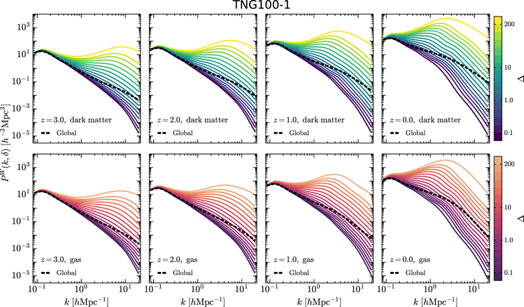
Figure 6. The env-WPSs of the dark matter (top) and baryonic gas (bottom) density fields of TNG100-1 at z = 3, 2, 1, and 0. The solid lines show the results for all the environments, as in Figure 5. In each panel, the global WPS (the dashed black line) is plotted for comparison.
Download figure:
Standard image High-resolution imageThe differences between the dark matter and gas fields can be precisely investigated by the env-bias and env-WCC, which are exhibited in the following.
4.2. The Env-bias of the Gas Relative to the Dark Matter
We now turn to consider the env-bias of the gas relative to the dark matter, the results of which are shown in Figure 7. We observe that the environmental bias function bW (k, δ) is almost independent of the scale and density environment on very large scales at all epochs. As the scale gets smaller, the environmental dependence of the bias becomes increasingly prominent. The main visible feature is the gas being most severely biased in the densest environment (Δ > 200), and at small scales for all redshifts, while the gas in the extreme underdense environment (Δ < 0.1) shows only minor bias. In more detail, we see that at z = 3, the env-bias value decreases monotonically as the density increases on scales 0.5 ≲ k ≲10 h Mpc−1, which is consistent with higher gas pressure in denser environments. Note that at this redshift, the suppression of the gas clustering is largely due to the gas pressure, while feedbacks play a minor role (see van Daalen et al. 2011; Chisari et al. 2018; Foreman et al. 2020). This monotonically decreasing trend of the env-bias with increasing density becomes weaker toward lower redshifts, and eventually, at z = 0, the env-bias hardly varies with the density on scales k ≲ 1 h Mpc−1, and even shows an upturn in densities of Δ ≳ 10 around the scale of k ∼ 3 h Mpc−1. We also notice that in these densities, the contours of bW ≳ 0.8 are shifted to smaller scales, compared to the case of z = 1. Since, at z < 3, the AGN feedback causes most of the suppression on scales of k ≲ 10 h Mpc−1, the redshift evolution of the env-bias in this scale range may reflect the AGN feedback efficiency in denser environments being reduced more severely than in less dense environments at lower redshifts. Hence, the gas in denser environments can be preferentially reaccreted to massive halos, confirming the findings of previous research. For example, by measuring the ratio between the total-matter power spectra in the Horizon-AGN and Horizon-noAGN simulations, Chisari et al. (2018) found that the clustering suppression at a scale of k ∼ 2 h Mpc−1 diminished slightly from z = 1 to 0, and ascribed it to the AGN feedback being less efficient in the most massive halos at lower redshifts. Foreman et al. (2020) measured the ratio of the bispectra between the hydro and dark matter–only simulation runs, and found that it was enhanced at z = 0, k ∼ 3 h Mpc−1 in TNG300-1, TNG100-1, and EAGLE, which was also due to less effective AGN feedback.
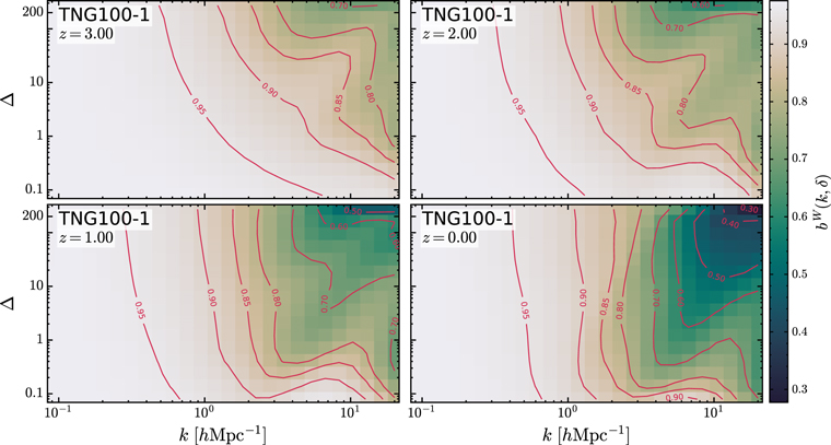
Figure 7. The env-bias of the gas with respect to dark matter, defined by Equation (13), at redshifts z = 3, 2, 1, and 0, measured from the TNG100-1 simulation. The bias is roughly constant on large scales, with bW ∼ 0.977 at z = 3, bW ∼ 0.967 at z = 2, bW ∼ 0.964 at z = 1, and bW ∼ 0.973 at z = 0.
Download figure:
Standard image High-resolution imageOn the galactic scales, i.e., k ≳ 10 h Mpc−1, the gas clustering is affected by the joint actions of gas cooling, star formation, and feedbacks, the former two of which are subdominant at the scales we are concerned with (k ≲ 20 h Mpc−1). As expected, the env-bias is approximately enhanced with increasing overdensity, indicating that denser environments experience more violent baryonic processes at the redshifts we consider. This result is consistent with the fact that denser environments host higher fractions of quenched galaxies (see, e.g., Hoyle et al. 2012; Moorman et al. 2016).
To determine whether our results depend on the particular galaxy formation model included in TNG100-1, we also measure the env-bias at z = 0 from the Illustris-1 and SIMBA simulations, which have similar box sizes to TNG100-1. In Figure 8, the upturn in densities of Δ ≳ 10 around the scale of 3 h Mpc−1 is also observed in SIMBA, which is even more obvious than in TNG100-1. Illustris-1 does not show this feature, which may be due to its overefficient AGN feedback for massive halos (Genel et al. 2014). For the same reason, the gas in Illustris-1 suffers the most severe suppression (particularly bW ∼ 0.2 in Δ ≳ 10 and at k ≳ 2 h Mpc−1) compared to the other simulations. Nonetheless, all simulations agree with the gas being more strongly biased in denser environments and on smaller scales at z = 0.
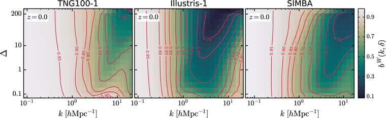
Figure 8. The env-bias of the gas at z = 0 measured from three simulations: TNG100-1, Illustris-1, and SIMBA.
Download figure:
Standard image High-resolution image4.3. The Env-WCC between the Dark Matter and the Gas
The time evolution of the env-WCC versus scale and density is shown in Figure 9. Overall, we see that the env-WCC is very close to 1 on large scales for all redshifts, which means that the distributions of the gas and the dark matter are highly coherent on large scales, and therefore the env-bias alone would be sufficient to derive the dark matter field from the gas field. As the scale decreases, the deviation of the env-WCC from unity becomes larger and shows a stronger environmental dependence, which is due to the redistribution of gas caused by baryonic physical processes.
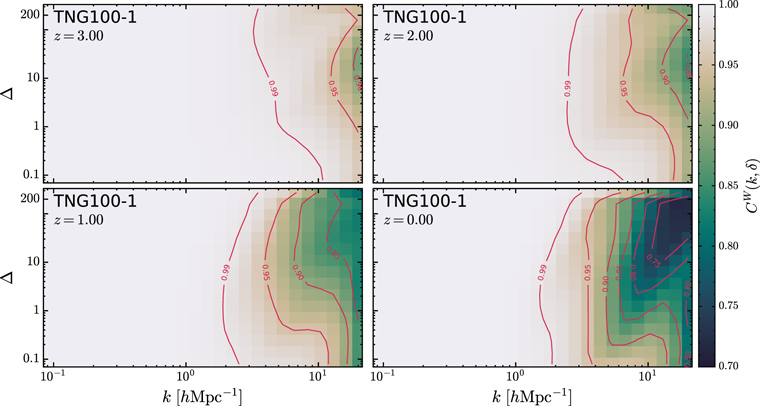
Figure 9. The env-WCC between the gas and the dark matter defined by Equation (14) at redshifts z = 3, 2, 1, and 0, measured from the TNG100-1 simulation. The env-WCC approaches unity on large scales, indicating that the gas and the dark matter are coherent with each other.
Download figure:
Standard image High-resolution imageAs revealed by the CW = 0.99 contour, the gas and the dark matter in the densest environment (Δ ≳ 200) always keep a very high correlation at scales k ≲ 3 h Mpc−1 for all redshifts. We notice that Farahi et al. (2022) reached a similar conclusion: in the TNG100-1 simulation, the correlation between the dark matter and gas density profiles of halos is very close to 1 on scales of r > R200, where R200 is the radius of a sphere whose enclosed average overdensity is 200 times the critical density. However, the 0.99 contour in less dense environments is shifted to larger scales at later times.
It can also be seen at z = 3 that the env-WCC shows an obvious nonmonotonic dependence on overdensity at scales of k ≳ 10 h Mpc−1, and is the lowest (CW < 0.90) between Δ ∼ 10 and Δ ∼ 40. This least-correlated region in the k − δ plot gradually expands to larger scales and lower-density environments with decreasing redshift, but is still concentrated in the environments of 0.1 ≲ Δ ≲ 200 (roughly the filaments and sheets). The gas always correlates tightly with the dark matter in the extreme underdense environments (Δ ∼ 0.1) from z = 3 to 0. Yang et al. (2021) also reported this feature and pointed out that the gas and the dark matter correlate more tightly in voids.
In Figure 10, we compare the env-WCC measured from TNG100-1 with those measured from Illustris-1 and SIMBA at z = 0. All of them show similar trends, with some discrepancies, possibly attributed to different galaxy formation models. Specifically, the gas correlates less with the dark matter in Illustris-1, and in the most underdense environments (Δ < 0.1) the env-WCC is even less than 0.80 at scales of 1 ≲ k ≲ 10 h Mpc−1, whereas this correlation between the gas and the dark matter is largely enhanced in TNG100-1, with an updated AGN feedback model. The characteristics of the env-WCC in SIMBA are intermediate between those in Illustris-1 and TNG100-1.
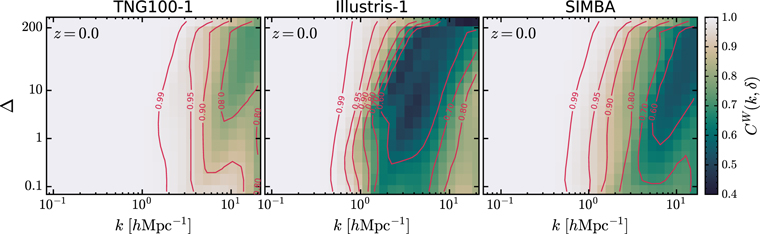
Figure 10. The env-WCC between the gas and the dark matter at z = 0 measured from three simulations: TNG100-1, Illustris-1, and SIMBA.
Download figure:
Standard image High-resolution image5. Discussion and Conclusions
In this paper, we propose three 3D wavelet-based statistical tools—(1) the env-WPS; (2) the env-bias; and (3) the env-WCC—which are defined as Equations (12), (13), and (14), respectively. These statistics are constructed from continuous wavelet coefficients, which simultaneously retain spatial and scale information. Therefore, we expect them to be able to quantify the density environment effects on the matter clustering at various scales. To verify this, we apply them to the dark matter and gas density fields of three state-of-the-art cosmological simulations: TNG100-1, Illustris-1, and SIMBA. To achieve a better spectral analysis, we use the CW-GDW as our analytic wavelet. Compared to the GDW used in our previous works (Wang & He 2021; Wang et al. 2021), this new wavelet has a higher resolution in the frequency domain, and therefore the global WPS based on it is much closer to the Fourier power spectrum, particularly on small scales (see Appendix).

Figure A1. Comparison of Fourier power spectra with global WPS. Top left: a 2D Gaussian random field with the power-law power spectrum P(k) ∝ k−2. Bottom left: the measured power spectra of the random field. Top right: a 2D projected dark matter density field at redshift z = 0 from TNG100-1, in a slice of width 75 h−1 Mpc and a thickness of 16 h−1 Mpc. Bottom right: the measured power spectra of the dark matter density field. In the two bottom panels, all WPS are normalized to fit the Fourier power spectrum.
Download figure:
Standard image High-resolution imageThis study has confirmed that the env-WPS, env-bias, and env-WCC are able to correctly characterize the dependence of the matter clustering on both the scale and the local density environment. The comparison of the env-WPSs between a Gaussian field and the present-day dark matter field shows that the env-WPS is fully capable of detecting non-Gaussianity (see Figure 5). Thus, it is promising that the env-WPS will be able to constrain cosmological parameters more tightly. The env-WPSs of the dark matter and gas exhibit similar features: they both converge to the global WPS at large scales, while at small scales they increase with increasing density at z = 3, 2, 1, and 0 (see Figure 6).
The differences of the spatial distributions between the gas and the dark matter are quantified by the env-bias and env-WCC (Figures 7–10). We notice that at redshift z = 3, the env-bias decreases with increasing density up to scales of a few times 0.1 h Mpc−1 in TNG100-1, indicating that the gas clustering is more suppressed in denser environments. At later times, when the AGN feedback effect is significant, this decreasing trend becomes progressively weaker, and eventually an increasing trend emerges at z = 0, i.e., the env-bias shows an upturn around k ∼ 3 h Mpc−1 and in Δ ≳ 10, which is also observed in SIMBA, but not in Illustris-1. This feature is likely a consequence of the decreased AGN feedback strength occurring in high-density environments at later epochs, which is supported by other research (Chisari et al. 2018; Foreman et al. 2020).
Moreover, by measuring the env-WCC in TNG100-1, we find that the dark matter and the gas in both the extreme dense (Δ ≳ 200) and underdense (Δ ≲ 0.1) environments always maintain very high correlation at all redshifts over a wide scale range, which qualitatively agrees with the findings in Farahi et al. (2022) and Yang et al. (2021). Particularly at the present epoch, the env-WCC is greater than 0.9 in densities of Δ ≳ 200 and Δ ≲ 0.1 at scales of k ≲ 10 h Mpc−1. However, the dark matter and the gas correlate less well in density environments of 0.1 < Δ < 200. A similar dependence is also observed in Illustris-1 and SIMBA, but with lower env-WCC values, possibly attributed to different galaxy formation models.
In general, our results suggest that density environment has a non-negligible impact on the characteristics of the matter clustering at low redshifts. Even on large scales of k ≲ 1 h Mpc−1, there is a visible density dependence for the env-bias. The env-WCC also shows density dependence up to scales of 2 h Mpc−1, and this is even larger in Illustris-1 and SIMBA. Consequently, by means of the env-bias and the env-WCC, the dark matter distribution should be predicted more precisely from the baryonic gas, which could be observed by upcoming sky surveys, e.g., CHIME (Bandura et al. 2014), HIRAX (Newburgh et al. 2016), and SKA (Bacon et al. 2020). In this sense, more cosmological simulations are needed to conduct a detailed census of the env-bias and the env-WCC for dark matter and gas. Furthermore, considering different gas phases, such as the warm–hot intergalactic medium or the diffuse intergalactic medium, may be more meaningful. Additionally, it is also important to investigate the differences between other tracers, such as halos and galaxies, and the dark matter density field from our wavelet statistics. These issues are left for future investigations.
The authors thank the anonymous referee for helpful comments and suggestions. The authors also thank the Illustris, IllustrisTNG, and SIMBA teams for their publicly available data.
P.H. acknowledges the support from the National Science Foundation of China (No. 12047569, 12147217), and from the Natural Science Foundation of Jilin Province, China (No. 20180101228JC).
Software: NumPy (https://numpy.org/), pyFFTW (https://github.com/pyFFTW/pyFFTW), SciPy (https://scipy.org/), powerbox (https://powerbox.readthedocs.io/en/latest/), Matplotlib (https://matplotlib.org/), Mayavi (https://docs.enthought.com/mayavi/mayavi/), Jupyter Notebook (https://jupyter.org/).
Appendix: Comparison between the Global WPS and the Conventional Fourier Power Spectrum in 2D
Until now, we have designed two kinds of wavelets, i.e., the GDW and the CW-GDW. Here, we check whether these wavelets could reproduce the Fourier power spectrum, which is important to do, since most works on matter clustering are done by Fourier analysis. To do this, we create a 2D Gaussian random field with a given power-law power spectrum P(k) = 0.1k−2 and make a comparison between its measured Fourier and global WPS, based on the anisotropic GDW and CW-GDW, which are computed by averaging all the wavelet coefficients over the whole space and the scale vector w with the same modulus. As shown in the bottom left panel of Figure A1, both the WPS with anisotropic GDW and CW-GDW, as well as the Fourier power spectrum, converge to the power-law power spectrum. Then we measure the Fourier and global WPS of the 2D density field of the dark matter at z = 0, the results for which are shown in the bottom right panel of Figure A1. It can be seen that all the power spectra have qualitatively the same shape and amplitude, except at large scales, which suffer from the finite-volume effect. Therefore, the WPS can also correctly characterize the matter distribution.
Nevertheless, the use of different analytic wavelets can lead to subtle differences in the results, which can be explained by the fact that the global WPS is the output of the Fourier power spectrum being smoothed by the square of a wavelet kernel (see, e.g., Wang et al. 2021). Obviously, the power-law spectrum is immune to such a smoothing operation, but, in general, the shape of the WPS will be smoother than the corresponding Fourier power spectrum. In our case, the GDW power spectrum is slightly lower than both the Fourier and CW-GDW power spectra on the scales k ≲ 3 h Mpc−1, and higher on k ≳ 20 h Mpc−1 for the highly nonlinear dark matter density field. This is due to the poor localization of the GDW in the frequency domain, as shown in Figure 1. Since the CW-GDW is more concentrated in frequency than the GDW, we see that the WPS based on the CW-GDW is closer to the Fourier power spectrum than that based on the GDW, especially on small scales. Finally, we compare the global WPSs, based on the anisotropic CW-GDW and the isotropic CW-GDW. As expected, they are almost identical.