Abstract
The interaction between the expanding supernova (SN) ejecta with the circumstellar material (CSM) that was expelled from the progenitor prior to explosion is a long-sought phenomenon, yet observational evidence is scarce. Here we confirm a new example: SN 2004dk, originally a hydrogen-poor, helium-rich Type Ib SN that reappeared as a strong  -emitting point source on narrowband
  images. We present follow-up optical spectroscopy that reveals the presence of a broad
  component with full width at half maximum of ∼ 290
  in addition to the narrow
  +[N ii] emission features from the host galaxy. Such a broad component is a clear sign of an ejecta–CSM interaction. We also present observations with the XMM-Newton Observatory, the Swift satellite, and the Chandra X-ray Observatory that span 10 days to 15 years after discovery. The detection of strong radio, X-ray, and
  emission years after explosion allows various constraints to be put on pre-SN mass-loss processes. We present a wind-bubble model in which the CSM is “pre-prepared” by a fast wind interacting with a slow wind. Much of the outer density profile into which the SN explodes corresponds to no steady-state mass-loss process. We estimate that the shell of compressed slow wind material was ejected ∼1400 yr prior to explosion, perhaps during carbon burning, and that the SN shock had swept up about 0.04
  of material. The region emitting the
  has a density of order
  .
.
1. Introduction
One of the major issues in supernova (SN) research is how stars that begin with ∼70% hydrogen on the main sequence are nearly or completely devoid of hydrogen by the time they explode. The hydrogen is lost by steady winds or bouts of mass loss or complex processes of binary star interaction involving one or more stages of common envelope evolution. In many proposed evolution scenarios some of the expelled hydrogen is expected to remain in a circumstellar medium (CSM). After the SN explodes, it will eventually run into that expelled matter after months, years, or even decades. Extensive mass loss has been associated with both Wolf-Rayet stars and luminous blue variables (LBVs; Smith 2014). Studying late-time interaction provides a means of probing the transition to and the duration of the Wolf-Rayet phase in massive stars and gaining a deeper understanding of the LBVs and other mass-loss phenomena.
There are several ways to study the late-time interaction of stripped-envelope SNe with previously shed material (for a review of interaction emission, see Chevalier & Fransson 2017). X-ray and radio emission are very likely signs of interaction and can provide mass-loss diagnostics. In the optical, the appearance of  emission at late times would be another sure sign of interaction; however, without a baseline measure of
  flux in the vicinity of an SN at early times, the detection of
  at late times could be ambiguous, as nearby H ii regions would also emit
  . Associating detected
  with interaction could be based on the following, in order of increasing level of conviction: (1) consistency with a point source; (2)
  luminosity above that of typical H ii regions (∼1037–1039); (3) variability; or (4) broadening of the
  line beyond that expected for an H ii region.
The first example of a hydrogen-deficient SN undergoing late-time collision with previously expelled envelope material was the Type Ib/c SN 2001em (Chugai & Chevalier 2006), characterized by late-time radio (Stockdale et al. 2004), X-ray (Pooley & Lewin 2004), and Hα emission (Soderberg et al. 2004). Late-time interaction was also seen in the Type Ia PTF 11kx (Dilday et al. 2012; Silverman et al. 2013; Graham et al. 2017).
Motivated by the example of 2001em, we began searching for late-time interaction in 2009 with a Cycle 11 Chandra X-ray Observatory proposal (PI: Pooley) targeting five old Type Ib/c SNe. Additionally, in order to increase the sample size substantially, we have been using the DIAFI imager on the Harlan J. Smith 2.7 m telescope at McDonald Observatory since 2014 February to search for evidence of delayed collision and excitation of  with narrowband filters, one near the expected redshifted wavelength of
  and another in an “off” band for calibration. Starting with a list of 3662 SNe, we have selected SNe Ia, and core-collapse SNe IIb, and SNe Ib that are closer than ∼35 Mpc and with decl. ≳ −30. This selection produced a list of 178 target SNe. Vinko et al. (2017) summarized our early results. With our narrowband imaging we have found evidence of
  at the location of the SNe for 13 of 99 events for which we have obtained and fully reduced the data through 2016. We confirmed the broad
  in SN 2014C, previously reported by Milisavljevic et al. (2015; see also Anderson et al. 2017; Margutti et al. 2017).
In our multi-epoch, narrowband imaging, we have found strong evidence of variability in three of 38 SNe observed more than once. Variability is sufficient, but not necessary, evidence of interaction. The CSM shock could be propagating through an extended medium generating roughly constant  flux as in the SN IIn 1988Z (Aretxaga et al. 1999). The strength of the Hα line is also an important clue if it is substantially larger than expected from an H ii region. An extreme example is SN 2005kl, which showed
 . Such a high
  luminosity strongly suggests the presence of CSM interaction. The most compelling
  evidence of interaction is the detection of the broadened
  emission.
Here we present optical spectra and X-ray observations of SN 2004dk that confirm this event to belong to the class of late-interacting SNe. Section 2 describes our observations of SN 2004dk. Section 3 presents some implications of our results. Conclusions and a look forward are given in Section 4.
2. SN 2004dk Observations and Analysis
2.1. Detection of Hα
SN 2004dk (a helium-rich, hydrogen-poor Type Ib) was detected in X-rays shortly after explosion (Pooley 2007) and by radio observations at later phases (Stockdale et al. 2009; Wellons et al. 2012). Early nebular spectra showed only a weak, narrow, unresolved Hα emission feature (Maeda et al. 2008; Shivvers et al. 2017). Our narrowband imaging on 2014 February 27, 2015 March 14, and 2016 June 9 provided a strong (signal-to-noise ratio > 50) detection of a point source at the position of the SN that suggested that the blast wave had finally reached the expelled H-rich envelope. SN 2004dk had an  luminosity of 1.5 × 1039
  , which is similar to that of SN 2001em (∼1039
  ). The lack of distinct Hα variability in our narrowband imaging left some doubt (Vinko et al. 2017). Our spectra taken in the spring of 2017 removed that doubt. In response to Vinko et al. (2017), Mauerhan et al. (2018) obtained and reported a broadened Hα profile of SN 2004dk. Here we present our narrowband imaging and spectral data and address the broader context in which they fit.
The late-time spectra on SN 2004dk were obtained with the Low Resolution Spectrograph 2 (LRS2) on the 10 m Hobby–Eberly Telescope (HET). LRS2 consists of two dual-arm spectrographs, covering 370–470 nm (LRS2-B UV), 460–700 nm (LRS2-B Orange), 650–842 nm (LRS2-R Red), and 818–1050 nm (LRS2-R Far-Red), with an average spectral resolution of R ∼ 1500 (Chonis et al. 2016).
For SN 2004dk, two spectra, taken on 2017 March 30 and 31, were acquired with the Red arm of LRS2-R, while a third spectrum was obtained with the Orange arm of LRS2-B on 2017 May 24. Figure 1 presents the full, combined LRS2-B + LRS2-R spectrum from 2017. The inset shows a blowup of the region of  in velocity space. We obtained another spectrum on 2019 June 21 which was virtually identical.
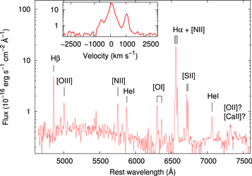
Figure 1. Combined LRS2 spectra of SN 2004dk showing the strong, broadened  and also Hβ, [O i], and He i. The latter are only seen in SN 2004dk and SN 2014C in our sample and give further support that an SN/CSM interaction is occurring in SN 2004dk 13 yr after the explosion. The inset shows the same spectrum in velocity space in the vicinity of
  .
.
Download figure:
Standard image High-resolution image2.2. Spectral Properties
Table 1 shows the list of features that are identified in the combined HET spectrum, based on the line identifications by Milisavljevic et al. (2015) for the interacting SN 2014C. It is seen that SN 2004dk and SN 2014C have many emission features in common: beside the strong hydrogen features, lines of He i, [O i], [O ii], [N ii], and [S ii] are present in the spectrum of both SNe. SN 2004dk lacks the broad Ca ii features that were strong in the spectrum of SN 2014C (Milisavljevic et al. 2015); in contrast, the He i features appear stronger in SN 2004dk. This could be attributed to somewhat different ejecta composition of the two events, or it could be due to the timing of the interaction.
Table 1. Emission Line Identification for SN 2004dk
| Ion/Feature | λ | FWHMa | FWHMib |
|---|---|---|---|
| (Å) | (Å) | (Å) | |
| Hβ | 4861 | 5.32 | 3.24 |
| [O iii] | 4959 | 5.12 | 3.31 |
| [O iii] | 5007 | 5.14 | 3.34 |
| [N ii] | 5755 | 8.40 | 3.83 |
| He i | 5876 | 8.45 | 3.92 |
| [O i] | 6300 | 7.84 | 4.20 |
| [O i] | 6364 | 9.20 | 4.24 |
| [N ii] | 6548 | 3.50 | 4.36 |

|
6563 | 6.55 | 4.37 |
| [N ii] | 6583 | 4.42 | 4.39 |
| [S ii] | 6716 | 4.02 | 4.48 |
| [S ii] | 6731 | 4.21 | 4.49 |
| He i | 7066 | 9.64 | 3.92 |
Notes.
aMeasured by Gaussian fitting. bComputed from instrumental resolution.Download table as: ASCIITypeset image
The full widths at half maximum (FWHMs) of the identified features (measured by Gaussian fitting) are also listed in Table 1. It is expected that the features that are associated with the expanding ejecta and the interacting region should be somewhat broader than those features that originate from the interstellar medium (ISM). Indeed,  the He i features, the [N ii] λ5755 and the [O i] λλ6300,6364 features appear somewhat more broadened than the other lines; however, all of these features are just barely resolved (the instrumental resolution being ∼4 Å), thus, their FWHMs do not fully reflect their intrinsic line width (except for
  and maybe He i; see below).
The flux ratios of forbidden lines of [N ii] and [S ii] can be used to estimate the electron density and temperature from the nebular-phase spectra (e.g., Osterbrock 1974). We measure the line flux ratio of (I(λ6548) + I(λ6583))/I(λ5755) ≈ 3.35 ±0.2 for [N ii]. Following Milisavljevic et al. (2015), we apply the TEMDEN task in IRAF to get a lower limit for the electron density of ≳2 × 105 cm−3, corresponding to Te ≲ 3.3 × 10⁴ K. A temperature of Te ∼ 104 K would imply Ne ∼ 7 × 105 cm−3. In contrast, the measured flux ratio of I(λ6716)/I(λ6731) ≈1.40 ± 0.1 for [S ii] would require Ne ∼ 22 cm−3 if the temperature were Te ∼ 104 K, which is similar to the densities of the outer regions in planetary nebulae (e.g., Osterbrock 1974). It is not possible to get a self-consistent solution from these two diagnostic line ratios, as the [S ii] ratio implies Te < 1.4 × 10⁴ K. This suggests that the formation of these features takes place at different locations along the line of sight: the [N ii] features that correspond to higher electron densities might be formed close to the shock-compressed CSM, see Section 3.3, while the [S ii] features more likely originate from the unshocked ISM, far from the SN.
2.3. Analysis of the Hα Profile
Figure 2 shows the  profile of our 2017 spectrum in contrast to a 2005 Keck spectrum (Shivvers et al. 2017), downloaded from the Weizmann Interactive Supernova Data Repository8
and scaled to match the strengths of the [N ii] 6548 and 6583 Å features of the new late-time spectrum. The Keck spectrum, taken with the Low Resolution Imaging Spectrograph (LRIS) with a resolution of ∼2000 that corresponds to ∼150 km s−1 around
profile of our 2017 spectrum in contrast to a 2005 Keck spectrum (Shivvers et al. 2017), downloaded from the Weizmann Interactive Supernova Data Repository8
and scaled to match the strengths of the [N ii] 6548 and 6583 Å features of the new late-time spectrum. The Keck spectrum, taken with the Low Resolution Imaging Spectrograph (LRIS) with a resolution of ∼2000 that corresponds to ∼150 km s−1 around  , shows slight broadening beyond instrumental. In our later spectra, the
  line shows a FWHM width of ∼290
  (see below). The line wings nearly overlap with the nearby lines of [N ii] at 6548 and 6583 Å. The collision ensues.
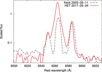
Figure 2. Spectrum of SN 2004dk obtained with HET LRS2 on 2017 March 30 compared to a much earlier spectrum obtained with Keck on 2005 May 11 (Shivvers et al. 2017). The  line is flanked by the two lines of [N ii] at 6548 and 6583 Å. The Keck spectrum shows only the narrow line corresponding to a nearby H ii region; the HET spectrum reveals clear broadening of the
  line, showing that ejecta/CSM interaction had begun.
Download figure:
Standard image High-resolution imageFigure 3 gives LRS2 spectra near  for three events. SN 2004ao shows
  in emission, but no signs of variability or broadening. SN 2014C, the youngest late-time interaction, shows both a narrow central unresolved component and a broad component, extending even beyond the [N ii] lines. SN 2004dk shows a definite but more modest broadening of the
  line, which may be expected for interaction occurring in an older SN.
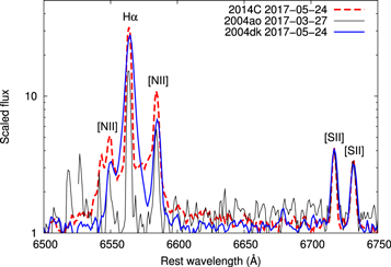
Figure 3.
 profiles of three SNe observed in our program. SN 2004ao (green) shows only instrumental broadening. SN 2004dk (blue) shows an intermediate level of broadening, distinctly more than instrumental. SN 2014C (red) shows both a central narrow, unresolved
  line and a substantially broader component. The two lines to the right are [S ii].
Download figure:
Standard image High-resolution imageMauerhan et al. (2018) estimated the FWHM of  from their Keck spectrum taken on 2017 May 29, nearly contemporaneously with our LRS2-B spectrum. They assumed that the
  line profile consists of a narrow (FWHM ∼130
  ) Gaussian and a broader (FWHM ∼400
  ) Lorentzian component with the narrow component having a factor of ∼2 higher amplitude than the Lorentzian one. Since the FWHM is affected by the amplitude ratio of the components, here we revisit this issue by refitting the
  line profile with a similar model; however, instead of fixing the amplitude of the Gaussian component or letting it float, we first fit the
  and the [N ii] λλ 6548,6583 features in the 2005 May 11 Keck spectrum with three Gaussians (Figure 4 top panel), then use the same amplitude ratio for
  /[N ii] λ6583 while fitting our combined LRS2 spectrum with the same three Gaussians plus a Lorentzian (Figure 4 lower panel). In so doing, we get a lower-amplitude Gaussian for the broadened
  feature and a higher Lorentzian component than Mauerhan et al. (2018). The FWHM of the Gaussian component turns out to be
 , while for the Lorentzian it is ∼290 ±4.5
  . Note that if we apply FWHM ∼ 130
  for the Gaussian component and fix its amplitude to be equal to that of the Lorentzian component, we recover the ∼400
  FWHM of the Lorentzian by Mauerhan et al. (2018).
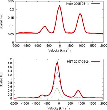
Figure 4. Top panel: fitting the 2005 Keck spectrum (red) with three Gaussians (black). Bottom panel: fitting the 2017 HET spectrum with three Gaussians plus a Lorentzian. The Gaussian and the Lorentzian components of  are plotted with green dotted and blue dashed lines, respectively. See the text for more details on the fitting.
Download figure:
Standard image High-resolution imageIf we consider the base of the  line profile instead of the FWHM, the width becomes ±1000
  . The total width at base is thus ∼2000
  . The FWHM is very sensitive to the amplitude of the Lorentzian, which depends on the spectral resolution and the amplitude ratio of the narrow and intermediate model components. It may be that the decelerated shock velocity is ∼1000–2000
  rather than ∼300–400
  . Note that the
  velocities we consider here could correspond to shock velocities, to intrinsic wind speeds, to broadening by electron scattering, or to the bulk motion of a cold, dense shell. We return to these issues in Sections 3.3 and 3.5.
From our 2017 HET spectra we measure  for the observed total
  flux above continuum and ∼6.7 ± 0.1 for the
  /Hβ flux ratio. Adopting D = 22.8 Mpc and AR = 0.342 mag for the distance and R-band extinction (Vinko et al. 2017), respectively, the total flux corresponds to an
  luminosity of L(
 ) = 1.63 ± 0.20 ×1039 erg s−1 or
  . This luminosity agrees well with that given in Vinko et al. (2017) within the uncertainties, and does not confirm the recent brightening (by a factor of 3) in the
  luminosity of SN 2004dk found by Mauerhan et al. (2018), even though our adopted distance of 22.8 Mpc is ∼10% larger than the one used by Mauerhan et al.. The flux measured from our 2019 spectrum is nearly identical to that of the 2017 spectrum. The
  light curve is shown in Figure 8.
2.4. Analysis of [N ii] λ6583 Line
Figure 5 gives a plot of the FWHM of Hα compared to the FWHM of the [N ii] λ6583 line for a number of events in our sample for which spectra have been obtained (see Table 4 in the Appendix). Most of the events show FWHM of both lines in the range 3–4 Å. Both SN 2004dk and SN 2014C (which falls off the top of the plot), are substantially more broadened than any of the others.
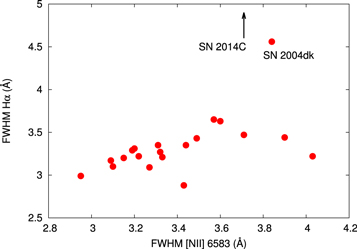
Figure 5. Plot of the FWHM of Hα compared to that of the [N ii] λ6583 line for a number of events in our sample. SN 2004dk and SN 2014C are distinctly more broadened, with SN 2014C falling off the plot, as indicated by the arrow.
Download figure:
Standard image High-resolution imageFigure 6 gives the ratio of the flux of [N ii] λ6583 to that of Hα as a function of the ratio of the fluxes of the two [N ii] lines, λ6548 and λ6583, for a number of events in our sample. SN 2004dk and SN 2014C are shown by both open symbols based on data obtained prior to the onset of late-time interaction and the solid symbols that represent the conditions after the onset of interaction. Note that the post-interaction  flux contains both the broad component formed in the ejecta behind the shock front as well as the narrow component that can originate both in the CSM in front of the forward shock and in the ISM of the host galaxy along the line of sight. The presence of the broad component is the primary cause of the strong decrease of the [N ii]/Hα flux ratio during the interacting phase. This is slightly different from the finding of Milisavljevic et al. (2015) who defined the flux ratio based on only the narrow Hα component. They found an increase of their flux ratio in SN 2014C during the interacting phase. Our definition, however, may be more suitable for objects like SN 2004dk in which the Hα profile cannot be easily separated into broad and narrow components.
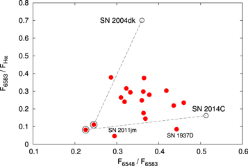
Figure 6. Ratio of the flux of [N ii] λ6583 to that of Hα plotted as a function of the ratio of the fluxes of the two [N ii] lines, λ6548 and λ6583, for a number of events in our sample. For SN 2004dk and SN 2014C, the open symbols represent data prior to late-time interaction and the solid points to data taken after the interaction had begun.
Download figure:
Standard image High-resolution imageFigures 5 and 6 suggest that both the FWHM comparison as well as the [N ii]/Hα flux ratio may serve as a diagnostic tool for identifying CSM interaction. For example, in Figure 6 the corresponding points for SN 1937D and SN 2011jm, the [N ii]/Hα flux ratio of which are below 0.1, are also highlighted. Although they have strong but still narrow Hα features, they are also candidates for CSM interaction.
2.5. Hα/Hβ Ratio
The  /Hβ ratio is usually higher in interacting SNe than in H ii regions. Under the conditions of Case B recombination, which is thought to be approximately valid for most H ii clouds,
  /Hβ ∼3.0–3.3 is expected (Osterbrock 1974), while in interacting SN flux ratios ∼6–10 is often observed.
Figure 7 shows the  /Hβ flux ratios of several interacting SNe including SN 2004dk. The flux ratio before the CSM interaction (or at the very beginning of the interaction in case of SNe that are discovered as Type IIn) is plotted on the horizontal axis, while the ratio during the strong interaction phase is shown on the vertical axis. Note that the superluminous SN 2006gy has two values, the lower point corresponding to the interaction phase around maximum light, while the other point corresponds to the late-phase, even stronger interaction. The sloping black line shows the 1:1 relation. It is seen that after the shock wave penetrates deep into the CSM, the
  /Hβ ratio always becomes higher than before. SN 2004dk (plotted with a filled circle) is no exception: it also shows increased
  /Hβ ∼ 6 measured from our late-phase spectrum (Figure 1) compared to the earlier value of ∼3.7 as seen from the 2005 Keck spectrum (Figure 2). Note that there seems to be an apparent correlation between the hydrogen flux ratios before and after the CSM interaction: SNe showing larger
  /Hβ in early phases tend to have higher flux ratio later. The very low number of events prevents a more definite conclusion. This could be an interesting subject for further studies.
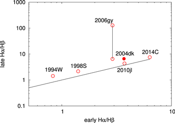
Figure 7. Ratio of the flux of  to that of Hβ in the late, strong-interaction phase plotted as a function of the ratio in early phases for several interacting SNe. The sloping black line represents a ratio of unity. SLSN 2006gy has two values connected with a vertical line. The lower point corresponds to the interaction phase around maximum light; the upper point corresponds to a later phase when the interaction is even stronger. SN 2004dk (filled circle) shows increased
  /Hβ ∼ 6 measured from our late-phase spectrum (Figure 1) compared to the earlier value of ∼3.7 as seen from the 2005 Keck spectrum (Figure 2).
Download figure:
Standard image High-resolution image2.6. X-Ray Properties
Since shortly after its discovery, SN 2004dk has been observed by several X-ray satellites. A log of the observations is given in Table 2.
Table 2. X-Ray Observations of SN 2004dk
| Satellite | ObsID | Date (UT) | Days After | Exp. |
|---|---|---|---|---|
| Discoverya | (ks) | |||
| XMM | 0164560801 | 2004 Aug 12.5 | 11.3 | 13.7b |
| Swift | 00035228001 | 2006 Jan 21.7 | 538.6 | 3.3 |
| Swift | 00035228002 | 2006 Jan 24.0 | 540.8 | 6.0 |
| Swift | 00035228003 | 2006 Jan 25.1 | 541.9 | 4.3 |
| Chandra | 11226 | 2010 Jan 18.8 | 1996.6 | 8.0 |
| Swift | 00088663001 | 2018 Apr 17.9 | 5007.8 | 0.6 |
| Swift | 00088663002 | 2018 Jun 30.3 | 5081.1 | 3.7 |
| Chandra | 21349 | 2019 Jan 11.9 | 5276.8 | 9.4 |
Notes.
a2004 August 01.19 (Graham & Li 2004). bFor MOS2; see the text for details.Download table as: ASCIITypeset image
SN 2004dk was observed by the XMM-Newton Observatory as a Target of Opportunity requested by D. Pooley. XMM-Newton took the observation 11 days after discovery on 2004 August 12 for 17.6 ks of exposure (Pooley 2007). We downloaded the ODF files from the XMM-Newton Science Archive and reprocessed them using the latest calibration files (as of 2018 June). We identified several large background flares in the data. After filtering these out, there were 7.9 ks of exposure in the pn camera, 12.7 ks exposure in the MOS1 camera, and 13.7 ks exposure in the MOS2 camera. We extracted source counts and spectra in the 0.4–8 keV band using a 15″ source region centered on the position of SN 2004dk and a 1′ source-free background region to the south. We obtained net counts of 17.5 ± 8.8, 8.6 ± 5.7, and 27.6 ±7.2 counts in the pn, MOS1, and MOS2 cameras, respectively, for a combined net count of 53.7 ± 12.7.
We fit all three source and background spectra simultaneously using the modified Cash (1979) statistic cstat in Sherpa (Fruscione et al. 2006). We first use an absorbed mekal model with absorption fixed at the value through the Milky Way in the direction of SN 2004dk of 
 , calculated from the Effelsberg–Bonn HI Survey (Winkel et al. 2016) using the online tool at the Argelander-Institut für Astronomie.9
The best-fit model, with a reduced cstat of 0.704, prefers a temperature at the upper limit of the model, kT = 80 keV. Adding an additional absorption component neither improves the fit nor lowers the best-fit temperature. An absorbed power-law model has a best-fit power-law index of 1.1 ± 0.3 for an identical reduced cstat of 0.704. Such a hard spectrum might indicate a non-thermal emission process, as expected for a Type Ib SN at early times (Chevalier & Fransson 2006). The unabsorbed 0.4–8 keV fluxes of the two types of best-fit models are the same within errors (Table 3) around
, calculated from the Effelsberg–Bonn HI Survey (Winkel et al. 2016) using the online tool at the Argelander-Institut für Astronomie.9
The best-fit model, with a reduced cstat of 0.704, prefers a temperature at the upper limit of the model, kT = 80 keV. Adding an additional absorption component neither improves the fit nor lowers the best-fit temperature. An absorbed power-law model has a best-fit power-law index of 1.1 ± 0.3 for an identical reduced cstat of 0.704. Such a hard spectrum might indicate a non-thermal emission process, as expected for a Type Ib SN at early times (Chevalier & Fransson 2006). The unabsorbed 0.4–8 keV fluxes of the two types of best-fit models are the same within errors (Table 3) around 
 , which corresponds to a luminosity of
 .
.
Table 3. X-Ray Spectral Modeling of SN 2004dk
| Observation | Model | PL Ind. | cstat/d.o.f. |
 (0.4–8 keV) (0.4–8 keV) |
|---|---|---|---|---|
| or kT | ( ) ) |
|||
| XMM (2004) | mekal | 80a | 3284.5/4664 |

|
| power law | 1.1
|
3284.4/4664 |

|
|
| Swift (2006) | mekal | 25
|
182.7/1518 |
 b
b
|
| Chandra (2010) | mekal | 80a | 506.7/1036 |

|
| power law | 1.3
|
506.6/1036 |

|
|
| Swift (2018) | mekal | 0.9
|
304.9/1518 |

|
| power law | 2.5
|
307.5/2528 |

|
|
| Chandra (2019) | mekal | 4.2
|
649.3/1036 |

|
| power law | 1.7
|
655.4/1036 |

|
Notes.
aModel maximum value. bUpper limit.Download table as: ASCIITypeset image
The Swift satellite observed SN 2004dk three times in 2006 January (around day 540) for a total X-Ray Telescope (XRT) exposure of 13.6 ks. Using a 10″ source region and 125 background region, we find four total counts in the source region, with an estimated 0.55 background counts in the region in the 0.4–8 keV band. Using the Bayesian method of Kraft et al. (1991), we calculate a 68.3% confidence interval of [1.7, 5.8] net counts and a 99.7% confidence interval of [0, 12.8] net counts. Because the 3σ-equivalent confidence interval includes zero, we regard this as a marginal detection at best and take the flux of the best-fit model as an upper limit. To obtain that flux, we extracted and simultaneously fit source and background spectra of the merged data using methods similar to those above. The best-fit mekal temperature is kT = 25 keV with no meaningful constraints because of the low quality of the data, and the unabsorbed 0.4–8 keV flux from this model is

 .
.
Chandra observed SN 2004dk on 2010 January 18 (around day 2000) for 8.0 ks with the telescope aimpoint on the Advanced CCD Imaging Spectrometer S3 chip as part of a program to investigate strong, late-time CSM interaction in Type Ib/c SNe, presumably due do the SN shock catching up to the previously cast-off hydrogen envelope (PI: Pooley). Data reduction was performed with the chandra_repro script, part of the Chandra Interactive Analysis of Observations (CIAO) software. We used CIAO version 4.9 and calibration database version 4.7.8. Using a 1″ source region and 1′ background region, we detected seven total counts in the source region, with an estimated 0.06 background counts in the region in the 0.4–8 keV band. We extracted and simultaneously fit the source and background spectra using similar methods as above. As with the earlier XMM data, these data prefer a best-fit mekal temperature at the limit of the model ( keV), which yields a reduced cstat of 0.489, but the temperature has a large uncertainty with a 68% confidence interval for kT of [4, 80 keV]. An absorbed power-law model has a best-fit power-law index of 1.3 ± 0.6 and has a reduced cstat of 0.489, also. The unabsorbed fluxes of the best-fit models are the same within errors (Table 3) around
 , which corresponds to a luminosity of
 .
.
Swift observed SN 2004dk again on 2018 April 17, but the XRT exposure was too short (687 s) to detect the SN in X-rays or to set an interesting limit, with only one count in the 10″ source region and an estimated background contribution of 0.02 counts. On the basis of our  detections, our team requested a longer Swift observation, which occurred on 2018 June 30 and had an XRT exposure of 3.7 ks. Merging the observations, we find five total counts in the source region, with an estimated 0.16 background counts in that region in the 0.4–8 keV band. Again using the Bayesian method of Kraft et al. (1991), we calculate a 68.3% confidence interval of [2.9, 7.5] net counts and a 99.7% confidence interval of [0.7, 14.9] net counts, indicating a secure detection. We extract and simultaneously fit the source and background spectra and obtain a best-fit mekal temperature of
  keV or a best-fit power-law photon index of 2.5 ± 0.9, which is markedly softer than previous X-ray observations. The unabsorbed fluxes of the best-fit models agree within errors (Table 3) around
 , which corresponds to a luminosity of
 .
.
Chandra observed SN 2004dk again on 2019 January 11 for 9.4 ks as part of a program to follow up on interesting  -emitting SNe from our DIAFI and HET programs (PI: Pooley). The data reduction, fitting procedures, source region, and background region are identical to the above. In the 0.4–8 keV band, we detect 58 total counts in the source region, with an estimated 0.06 background counts. The best-fit mekal temperature is
  keV. A power-law fit gives a photon index of 1.7 ± 0.2. The unabsorbed fluxes of the best-fit models are the same within errors (Table 3) around
 , which corresponds to a luminosity of
 . SN 2004dk brightened by a factor of ∼8 between the Chandra observation in 2010 and that in 2019.
The X-ray light curve is plotted with our  light curve and radio data reported in Wellons et al. (2012, see below) in Figure 8.
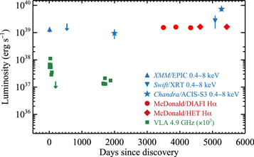
Figure 8. Multiwavelength light curve of SN 2004dk. X-ray measurements are shown in blue with symbols indicating the satellite (the upper limit is from Swift).  measurements are shown in red; circles indicate results from our narrow-band imaging (Vinko et al. 2017), and the diamond is from our HET spectra reported here. Green squares are based on 4.9 GHz radio flux densities from the Very Large Array reported by Stockdale et al. (2009) and Wellons et al. (2012) and converted to luminosities assuming a flat spectrum and 100 MHz bandpass.
Download figure:
Standard image High-resolution image3. Discussion
3.1. Early CSM Interaction
Wellons et al. (2012) observed the radio flux from SN 2004dk from about 8 days to about 80 days after explosion and fit its characteristics with a self-absorbed synchrotron model. They found that the radio emission was consistent with the propagation of the SN shock into a steady-state wind with a density profile scaling as ρ ∝ r−2. They concluded that the electron density at the onset of the interaction was ne ∼ 2.2 × 10⁴ e− cm−3 at a radius ∼5 × 1015 cm and that the shock propagated at a mean velocity of 0.2c = 6 × 10⁴  over the first 80 days. For a wind velocity of 1000
  characteristic of a stripped core, they deduced a mass-loss rate of
 yr−1. They also determined an upper limit to the radio flux about 200 days after explosion that was consistent with the expected decline in a steady-state wind with the properties they had deduced that would have been less than the observed limits by about a factor of 3.
Our XMM-Newton observation around day 11 reveals a hard spectrum, indicating that thermal emission is probably not the source of the X-ray photons. Rather, as suggested by Chevalier & Fransson (2006), synchrotron and inverse Compton processes are likely responsible for the early X-ray and radio emission in Type Ib and Ic SNe. A model X-ray light curve, presented in Figure 1 of Chevalier & Fransson (2006), gives a predicted  of
of  at an age of ∼11 days and assumes an optical light curve like that of SN 1994I. Comparing the absolute V-band light curves of SN 1994I and SN 2004dk given in the Gold Sample of SN Ib/c by Drout et al. (2011, their Figure 7), SN 2004dk peaks about 1 mag more luminous than SN 1994I. Our measurement of
 at t = 11 days is ∼3 times higher than the model of Chevalier & Fransson (2006). Since the optical photons are inverse Compton upscattered to X-ray energies at early times, the X-ray flux should scale with the optical. Since both our
  measurement and the peak optical luminosity of 2004dk are a factor of ∼3 higher than 1994I, the early X-ray emission detected by XMM-Newton is likely explained by the synchrotron + inverse Compton model of Chevalier & Fransson (2006). This conclusion is consistent with the non-thermal origin of the contemporaneous radio emission.
As a consistency check, we can estimate the bolometric luminosity of the shock at this time. Assuming spherical symmetry, the bolometric luminosity of the forward shock would be

Assuming 
 yr−1, vw = 1000
  , and the shock to propagate at 6 × 10⁴
  gives Lbol = 4.1 ×1041 erg s−1. This estimate of Lbol is comfortably in excess of the observed X-ray luminosity at this epoch. As a further check, we can estimate the X-ray luminosity if the X-rays were produced by a thermal mechanism,
  , where Λ is the cooling function and V the radiating volume. We find
  estimated in this way to be of order 1033 erg s−1, far below the observed X-ray luminosity, giving further support to the non-thermal model for the early X-ray emission seen by XMM-Newton at 11 days. The later emission seen by Chandra at 2000 days is ∼102 higher than predicted by the model of Chevalier & Fransson (2006), indicating that another emission process is at work at late times.
3.2. Late-time “Rebrightening”
Stockdale et al. (2009) and Wellons et al. (2012) detected radio emission from SN 2004dk 1660 days or 4.5 yr after the explosion with a flux that was comparable to the 200 day upper limit. Wellons et al. (2012) termed this later detection a “rebrightening” since it was about 40 times the flux expected from extrapolation of the steady-state wind model that fit the earlier detections. The radio rebrightening was attributed to the collision of the forward shock with denser circumstellar material, and our Chandra measurement of a high  around day 2000 supports this interpretation. The beginning of the interaction of the ejecta with denser CSM material presumably occurred some time before the radio rebrightening was detected.
The CSM detected early likely arose from the fast wind from a stripped core, as discussed above. One hypothesis is that the rebrightening occurred when the shock impacted the hydrogen-rich matter we detect; the radio rebrightening could represent mass that had been lost at a much earlier phase that was hydrogen rich and presumably ejected by a different physical process that was not necessarily a steady-state wind. Mauerhan et al. (2018) proposed a model in which a fast wind blows a low-density bubble interior to a denser shell ejected at an earlier phase. The outer shell could be the material from a slower wind compressed by the later, faster wind (Dwarkadas 2005, 2011; Dwarkadas et al. 2010) or material shed in a different process, for instance by common envelope evolution or a burst of episodic mass loss.
Assuming that the epoch of the radio rebrightening represents an upper limit to the time when the shock began to interact with denser, circumstellar material, the boundary of the outer denser material associated with the rebrightening would be at  cm, where rrb is the radius of the shock at the time of rebrightening and
  is the shock velocity in units of 104
  . Adopting the shock velocity deduced by Wellons et al. (2012),
  yields rrb ∼ 8.4 × 1017 cm. For a self-similar shock for which v ∝ t(s−3)/(n−s) where n = 10 is the density slope in the SN ejecta (estimates range from 7 to 12) and s = 2 is the density slope of the CSM, the velocity will scale as
  . For this mild deceleration, the shock would decelerate from
  at 80 days to
  at 1600 days.
This boundary to denser material must be greater than 5 × 1015 cm, given the early radio observations of Wellons et al. (2012). A larger lower limit is given by the deduction of Wellons et al. that the average velocity over the first 80 days is 0.2 c. This gives a lower limit of 4 × 1016 cm.
If the density continues to fall as ρ ∝ r−2 beyond the region of rebrightening, the bolometric luminosity from Equation (1) would decline as t−3/8. At 2000 days, the bolometric luminosity would be reduced by a factor of about 0.14 compared to that at 11 days and would still be comfortably more than the X-ray luminosity measured by Chandra at that later time, 9.5 × 1038  . If the density fell off less steeply, the bolometric luminosity would be even higher. We will revisit these issues in Sections 3.4 and 3.5.
SN 2004dk was 3500 days or 9.6 yr old when we first detected it as a bright  point source on 2014 March 27 (Vinko et al. 2017). The rebrightening was 1700 days earlier, and the collision with material denser than the inner fast wind must have occurred earlier than that. The shock had at least 5.1 yr to decelerate in the relatively denser material after the epoch of radio rebrightening. During this interval, the shock would have propagated with a mean velocity between the velocity we deduce at rebrightening,
  , and that we deduce from the
  line width,
  . This would put the location of the shock at the epoch of the first broadened
  detection at 4.4 × 10¹⁵ to 5.9 × 1017 cm beyond the location of the rebrightening. The latter is almost surely an upper limit, so the implication is that the shock had not propagated substantially in radius from the time of the rebrightening.
Using a model of synchrotron self-absorption to analyze the early radio data of SN 2004dk, Wellons et al. (2012) concluded that the electron density at the early epoch was ne,0 ∼ 2.2 ×10⁴ e− cm−3 at a distance of  cm from the progenitor. They determined that the radio flux at the time of the rebrightening increased by a factor of ∼40 compared to an extrapolation of the early radio data based on a steady-state wind. Assuming the magnetic field and the shock Lorentz factor, and hence a characteristic synchrotron frequency, do not change (assumptions that might be questioned), and equipartition of the magnetic field in the shock, Wellons et al. argued that the synchrotron radio flux scales as
  , where ve is some mean electron velocity. The increase in flux at the epoch of rebrightening thus suggested that the electron density of the CSM was higher by a factor of 401/2 ∼ 6.3 compared to that obtained by extrapolating the earlier model to the location of the rebrightening. Assuming a constant mass-loss rate at constant velocity, the density at the location of the rebrightening can be expressed as

For  , this gives ρrb ∼ 1.5 × 10⁻²³ vsh,4−2 g cm−3 or ρrb ∼ 10−24 g cm−3 for vsh,4 = 4. If the density jumps by a factor of 6.3, the density would then be ρsh ∼ 6 × 10⁻²⁴ g cm−3.
3.3. Constraints from the Late-time Hα Luminosity
The  luminosity provides constraints on the density of the material emitting that flux. Taking the Case B recombination rate per unit volume to be nenpαB(T) with ne = np for pure hydrogen and the recombination coefficient for pure hydrogen to be (Osterbrock 1974)

where T4 is the temperature in units of 104 K, the recombination  luminosity for a constant-density cloud of radius r is then

With  erg, and np = ρN0, this can be expressed as

If the recombination flux comes from a thin shell, then the corresponding expression would be

where  is the fractional thickness of the thin shell.
In Section 2.4 we found the  flux for SN 2004dk to be 1.63 × 1039 erg s−1 at 4626 days. Mauerhan et al. (2018) give the estimated
  luminosity for several related events as 2.5 × 1039 erg s−1 at 1327 days for SN 2014C, 1.3 × 1039 erg s−1 at 2218 days for PTF11iqb, and 2.2 × 1038 erg s−1 at 1883 days for SN 2009ip. Note that all these values are rather uncertain because of the uncertain distances and flux calibration issues.
The location of the  emission in each of these cases is uncertain. The propagation of the SN shock is uncertain since the propagation velocity depends on the possible complex CSM density distribution (see Section 3.5). For a characteristic average shock speed of 104
  propagating for several thousands of days, the typical scale would be a few times 1017 cm for these four objects. The characteristic distances would be 4.0 × 10¹⁷vsh,4 for SN 2004dk, 1.2 × 10¹⁷vsh,4 for SN 2014C, 1.9 × 10¹⁷vsh,4 for PTF11iqb, and 1.6 × 10¹⁷vsh,4 for SN 2009ig, where vsh,4 is the shock velocity in units of 104
  . From Equation (6), we can then write the density as

For each of the SNe, the quantity 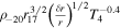 is then 67 for SN 2004dk, 83 for SN 2014C, 60 for PTF11iqb, and 25 for SN 2009ig. Note that the
  luminosity must be coming from the outer dense shell. The density we derive for the region between rrb and the outer shell, ∼10−23 g cm−3, is far too low to generate the flux we detect.
The resulting CSM densities are rather insensitive to temperature, but are sensitive to the location of the  emission and to the potential thinness of any shell emitting
  . If the shell had a thickness only ∼0.01 the radius of the shell, the densities would all be larger by an order of magnitude. It is then difficult to compare the various events quantitatively because the radius and shell thickness could be quite different for the various events. Given the uncertainties in the values of the scaling parameters, the densities deduced in this manner are considerably higher than that deduced above for SN 2004dk based on the radio synchrotron emission, ρ−20 ∼ 5.5 × 10⁻³, just interior to the density jump represented by the rebrightening. The deduced densities are roughly comparable to the mean density of molecular clouds. The density we deduce for SN 2004dk is, however, consistent with the density estimated from [N ii] emission in Section 2.2, ρ−20 ∼ 30–120, for an ionized plasma.
Beginning at 3500 days, we observed SN 2004dk with narrowband filters for 830 days with no substantial change in  flux (Vinko et al. 2017). If the Lorentzian FWHM of ∼300
  that we measure for
  corresponds to a shock speed, this implies that the conditions in the shell were nearly constant over a radial scale of
  cm. This length scale could be nearly an order of magnitude larger if the base width of the
  line were used, but the corresponding displacement would still be small compared to the radius, ∼1017 cm. Given that the radius could not have changed substantially over this timescale, and assuming that the shell thickness did not change substantially, then Equation (6) suggests that the quantity
  is nearly constant over this time interval. Even that is suspect, given the uncertainties in clumping, asymmetry, and other factors. This argument would not apply if the 300
  is the cold dense shell (CDS) velocity, not the shock velocity. Mauerhan et al. (2018) argued that the
  flux may have increased in just the last 1000 days after Vinko et al. (2017); however, independent measurements presented in Section 2 do not confirm such a change in the flux of
  .
.
3.4. Constraints from Late-time X-Ray Emission
It is difficult to estimate the fraction of the bolometric luminosity that will be emitted in X-rays as it was to estimate the  flux, as just illustrated. The X-ray luminosity will depend on the optical depth among other factors. For SNe IIn, the X-ray flux can be substantially more than the flux in
  in some cases, but substantially less in others (Branch & Wheeler 2017, Chapter 14). In the case of 2004dk, they are comparable for a while, but the X-rays have risen substantially by ∼5000 days, while the
  has remained constant (Figure 8). This clearly shows that the X-rays could not give rise to the
  flux. The
  cannot arise from a medium ionized by X-rays.
The standard picture of X-rays produced by a reverse shock in CSM interaction is of limited applicability here because we have the SN ejecta first interact with a lower-density CSM and then a higher-density CSM. The Chandra observation of high  at ∼2000 days confirms the onset of late-time interaction, as seen in the radio. It does not provide additional constraints on the onset of the late-time interaction, but may provide some constraints on densities and velocities in the context of a correct physical model.
The X-ray flux from the Swift observation around 5100 days and Chandra observation around 5300 days seems softer and hence may be due to thermal processes. If so, there is then a constraint on the shock velocity because if the velocity of the shock in the shell is too low, we would not expect any X-ray emission at all. One would need 400  to get the temperature above 106 K, and 500
  or more to get even very soft X-ray emission in the 0.2–0.2 keV band. The FWHM of the
  may be too low to produce thermal X-rays, although the full width of the base of the line (2000
  ) would represent a sufficient velocity; this may indicate that the base of the
  line gives a better indication of the shock velocity than the FWHM. Another complication is that the shell we envisage might be clumpy. It could be that the shock propagates more rapidly in more rarified regions and slower in denser regions and that the thermal X-rays are not produced in the same region as the
  although both are produced in the dense shell. There are several ways to break spherical symmetry, but that is beyond the scope of the current paper; we will continue to acquire more observations and address this issue in a future publication.
3.5. Wind-bubble Model
The density in the vicinity of the rebrightening event derived in Section 3.2, ρ ∼ 5.5 × 10⁻²³ g cm−3, is incommensurate with that derived from the  luminosity in Section 3.3, ρ ∼ 2.6 × 10⁻¹⁹ g cm−3 (modulo various scaling parameters). In addition, the estimated mass-loss rate that could give the density jump estimated by Wellons et al. (2012) in Section 3.2,
 yr−1, seemed unphysically low for plausible mass-loss processes that could produce a slow wind or other processes at the appropriate radius. These apparent discrepancies may be accommodated in the context of a model in which the SN explodes in a CSM that has been previously structured by interacting fast and slow winds, a wind-bubble model.
Early numerical models of the interaction of a wind with the ISM, including effects of conduction, were given by Weaver et al. (1977). Chevalier & Liang (1989) and Tenorio-Tagle et al. (1991) explored models of an SN exploding into such a “prepared” CSM. Dwarkadas (2005, 2011) and Dwarkadas et al. (2010) investigated an SN exploding in a CSM in which a fast wind interacted with a previous slow wind which itself interacted with the surrounding ISM. This is a natural environment in which to consider our observations of SN 2004dk.
From the inside out, the structure of the CSM in a wind-bubble model has an inner fast wind that is plausibly due to a nearly steady-state wind from the stripped-envelope, hydrogen-deficient progenitor. In this case, the inner CSM has the characteristic density profile  . This inner wind structure ends at a termination shock where the freely expanding fast wind is shocked by the reverse shock resulting from the fast wind interacting with the outer, slower wind. This shock results in a density jump of about a factor of 4 for a strong shock in a perfect monatomic gas. Beyond the termination shock, the density slowly rises to the inner boundary of the contact discontinuity between the inner fast wind and the outer slow wind.
Under common circumstances, the matter in the vicinity of the outer shock where the fast wind collides with the slow wind will be strongly radiative, leading to cooling and the formation of a CDS. At that point, the CSM density typically jumps by a factor of order 103. If the CDS forms from the interaction of two steady-state winds, the resulting velocity of the CDS is constant,  (Weaver et al. 1977; Dwarkadas 2005). Beyond the CDS, the forward shock of the wind interaction propagates into the outer portions of the dense, slow wind (Dwarkadas 2005, Figure 4).
Note, critically, that the density structure between the termination shock and the CDS corresponds to non-homologous structure and to no specific mass-loss rate. The resulting overall density structure is the result of neither a steady-state wind nor homologous expansion; it is a characteristic of interacting flows.
Note also that if the fast inner wind is hydrogen deficient then so also is the region of the fast inner, freely expanding wind and the region between the termination shock and the CDS. In this picture, the  emission we detect cannot be from near the termination shock, but must be from within or beyond the CDS, presuming the outer slow material to be of solar composition.
This basic picture can be complicated by a number of factors, including Rayleigh–Taylor instabilities, as discussed by Dwarkadas (2007), but captures the essence of the situation. The SN then explodes into the rather complex “prepared” CSM.
When the SN explodes, the ejecta shock runs relatively quickly through the inner freely expanding wind, somewhat more slowly through the nearly constant-density region between the termination shock and the CDS, and then very slowly through the CDS before breaking out into the outer, undisturbed slow wind. The passage of the SN shock substantially changes the density structure of the medium. When the ejecta shock hits the termination shock, a transmitted shock is sent forward into the nearly constant-density portion of the wind bubble until it encounters the CDS. A new reflected shock propagates back into the ejecta, overcoming the original reverse shock and continuing into the ejecta. The original wind termination shock is obliterated.
There is still a jump of a factor of several in density at the location of the new reflected shock. This jump is thus very reminiscent of the apparent jump in density at the epoch of the radio rebrightening 4.5 yr after the explosion of SN 2004dk. The increase in density is likely to be a factor of 4 representing the jump over a strong shock rather than the uncertain factor of 6.3 formally derived by Wellons et al. (2012).
Given the basic structure of the CSM prepared by the interaction of fast and slow winds, we can outline the resulting characteristics of the matter in the wake of the subsequent SN shock. We normalize to the initial condition presented by Wellons et al. (2012): electron density ne ∼ 2.2 × 10⁴ e− cm−3 at a radius ∼5 × 1015 cm and a mean velocity of 0.2c = 6 ×10⁴  over the first 80 days. As noted in Section 3.2, the shock is likely to have slowed to a velocity of
  after 1600 days. We take a mean velocity during this interval to be
  Adopting this shock velocity gives the location of the rebrightening as rrb ∼ 6.9 × 1017 cm.
From Equation (2), the density at the outer limit of the fast wind at rrb will be ρrb− = 6.3 × 10⁻²⁵ g cm−3. Assuming the strong shock at the transition from the fast to the outer slow wind results in a density jump of a factor of 4, the density just beyond this jump at rrb will be ρrb+ = 2.5 × 10⁻²⁴ g cm−3.
Across the presumed density discontinuity, pressure, and hence ρv2, is nearly constant. The shock velocity just beyond the density jump will then decrease by a factor of 2 to vsh,4 ∼ 2. For a fast wind of constant mass-loss rate colliding with a slow wind of constant mass-loss rate, the density profile between the transition shock at rrb and the outer dense shell will be nearly constant. A similarity solution then gives vsh ∝ t−3/n = t−0.3. The velocity of the shock will then decelerate in this medium as

where we have taken the epoch when the shock hits the shell, tshell, to be the time of our first observation of bright  . By the time the shock hits the boundary of the dense outer shell, it will thus have decelerated to a velocity of
  .
.
Likewise, a similarity solution in a constant-density medium gives the location of the shock to be rsh ∝ t(n − 3)/n = t0.7. The location of the shock in the constant-density medium when the shock arrives at the boundary of the outer dense shell is then approximately

With rrb ∼ 6.9 × 1017 cm, the location of the inner edge of the shell is thus estimated to be at rshell ∼ 1.2 × 1018 cm.
When the shock enters the outer dense shell, we can again invoke the behavior across a density discontinuity, ρv2 ∼ constant so that the velocity within the shell, vin, can be written

We take the estimate of the density within the dense shell as constrained by the  luminosity (Equation (7)) to be

and hence, with the density on the exterior of the density jump at the rebrightening of  g cm−3, we find

This result is roughly compatible with the FWHM that we measure for the  line. Note that δr/r must be considerably less than unity to comport with the thin shell approximation we have implicitly made in the analysis.
The properties we derive for SN 2004dk are thus qualitatively consistent with a wind-bubble model in which the SN exploded into a CSM comprising the previous interaction of fast and slow winds.
3.6. The Slow Wind
If the outer, denser CSM material had been ejected as a wind at about 10  as might be characteristic of a red supergiant or a common envelope, and the shocked material lay at about the distance we estimate for the outer dense shell, rshell ∼ 1.2 × 1018 cm, then this material would have been ejected about 48,000 yr ago, perhaps during helium core burning. Other matter from this slow wind could have been ejected earlier and be at larger radii, but we have no constraints on that. Another component of the slow wind would have been ejected later, but then swept up by the even later, fast wind. When the fast wind turns on, it compresses the slow wind, forming the dense shell. As the fast wind continues, it sweeps up more slow wind material. The mass of the shell increases with time as more slow wind material is swept up, but the velocity of the shell is nearly constant. A similarity solution (Dwarkadas et al. 2010, Appendix) gives

With 
 yr−1 and vfast = 103
  from Wellons et al. (2012),
 yr−1, a typical mass-loss rate for a red supergiant, and vslow = 10
  , we find vshell ≈ 270
  and the time for the shell to reach its current distance of 1.2 × 1018 cm to be 1400 yr. The onset of the fast wind would thus correspond roughly to core carbon burning, long before oxygen or silicon burning, depending on the zero-age main-sequence mass of the progenitor.
From momentum conservation, the CSM mass that can decelerate a mass of shocked material Msh from v0 to v1 is

for  (e.g., Chugai & Chevalier 2006). If v0 ∼ 104
  and v1 ∼ 300
  this gives a mass ratio of MCSM/Msh ∼ 32.
We can deduce the amount of slow, dense wind swept up by the fast inner wind at the location of the dense shell,  , as
, as

assuming rshell = 1. 2 × 10¹⁸, 
 , and where we have scaled the presumed slow wind to
 yr−1. This is a plausible amount of mass to be swept up from a red supergiant wind, given uncertainties about the mechanism. The total mass ejected in a red supergiant wind or other process could be even larger but remains unshocked and undetected.
4. Conclusions and Future Work
We have presented late-time optical and X-ray observations and analysis of SN 2004dk, demonstrating that the SN is now strongly interacting with mass loss shed from the progenitor star prior to core collapse. The line of  is broadened to a FWHM of about 300
  . In addition, SN 2004dk shows a ratio of
  to Hβ of about 6, far stronger than typical H ii regions and another indication of interaction. SN 2004dk also shows evidence for [O i] and He i that may be heated or excited by the interaction.
We have presented XMM-Newton, Chandra, and Swift observations that show a remarkably constant luminosity close to that emitted by  . We argue that the early X-rays at 11 days and those at 2000 days are likely to be non-thermal, but that the X-rays detected by Swift and Chandra after 5000 days are probably thermal. We have no ready explanation for why the thermal and non-thermal luminosities are so similar, but note that other long-lasting interactions have also produced nearly constant X-ray luminosity. The detection of thermal X-rays later than 5000 days implies a shock velocity greater than several hundred
  and likely more than ∼1000
  .
.
We present a wind-bubble model in which the CSM is “pre-prepared” by a fast wind interacting with a slow wind. This model allows a reasonable estimate of the velocity manifested by the broadened  in terms of the early mass loss and the shock velocity suggested by the radio observations. We estimate that the slow wind material currently in the vicinity of the dense shell was blown about 48,000 yr ago, perhaps during the red supergiant phase of core helium burning, and that the fast wind started about 1400 yr ago as the star ejected the last of its hydrogen envelope, perhaps during carbon burning. In this interacting-wind model, much of the outer density profile into which the SN explodes corresponds to no steady-state mass-loss process. The dense shell arises naturally in a model of interacting winds and does not require a special epoch of temporarily enhanced mass loss (Shiode & Quataert 2014; Fuller 2017; Nance et al. 2018); it is just a fast, low-density Wolf-Rayet wind interacting with a red supergiant wind.
In numerical models, when the forward shock breaks out of the CDS, its velocity increases to in excess of 1000  before decreasing over a long timescale as it continues to propagate into the undisturbed outer slow wind. The late-time thermal X-rays may be consistent with that velocity as is the width of the
  line at its base. If the shock has propagated beyond the CDS, radiation from the forward shock could photoionize the matter in the undisturbed wind. Given that the X-ray and
  are of nearly equal luminosity and that the X-ray emission has risen with no corresponding rise in
  , this cannot be an explanation for the
  flux. The absence of strong narrow emission lines might suggest the forward shock has not yet broken out of the CDS for SN 2004dk, but evidence for this may be hidden in unresolved lines. The shock and associated excitation structure may be more complex if the former is propagating through a turbulent, clumpy medium. It may be that the relatively narrow
  is generated from dense clumps, and the flux in the base of the line and the thermal X-rays are produced in more rarefied material between the clumps. The X-rays could also be produced by the reflected shock from the CDS going into a somewhat lower-density region inside of the shell.
We do not know when SN 2004dk began producing  luminosity. It showed no obvious variation in
  flux in our narrowband imaging, but it may be in a long-lived phase of interaction with slow evolution. We note that other events in our sample show the opposite effect; they show variable
  flux, yet no obvious sign of line broadening.
It is interesting to know how SN 2004dk compares and contrasts with other stripped-envelope core-collapse events, especially SN Ib, that have and have not displayed evidence of late-time interaction with hydrogen-rich material. A systematic comparison is the subject of a later paper, but a comparison of the  flux of few related objects—SN 2004dk, SN 2014C, PTF11iqb, and SN 2009ig—at various phases ranging from 1300 to 4600 days is given in Section 3.3. Characteristic shell radii are ∼1017 cm. The density of the region emitting
  is rather insensitive to temperature, but is sensitive to the location and the assumed thickness of the shell.
The event that triggered this particular line of investigation for SNIb/c was SN 2001em. SN 2001em may have been discovered before maximum light (Chugai & Chevalier 2006). Interaction was detected in the radio about 770 days after the estimated date of explosion, and X-rays were detected on day 937 at the level of  . Hydrogen emission was observed on day 970. These timescales are commensurate with those of SN 2004dk, but, as for SN 2004dk, the interaction must have begun at an indeterminate time prior to these observations. Chugai & Chevalier (2006) adopt a model in which a dense, massive, 2.7
  , circumsteller shell is formed by a period of very high mass loss, 2–10 × 10−3
  yr−1, followed by a fast wind which swept up the lost mass into a dense shell and accelerated it. They derive a rather modest final velocity of the shell prior to the explosion of ∼30–50
  . In the wind-bubble model we invoke here, the velocity of the shell is essentially constant as given by Equation (13) for which we find the shell velocity for SN 2004dk to be 270
  . Given the similarity of the models used for each SN, it is likely that the differences in derived shell velocities and densities are related to the different X-ray luminosities of the two SNe and possibly to different timescales for the onset of the interaction with the shell.
Of particular interest is the well-studied case of SN 2014C. Interaction was already conspicuous in optical spectra of SN 2014C on day 113 when it emerged from solar hiatus (Milisavljevic et al. 2015; Margutti et al. 2017), and the radio brightened in that event at about 200 days (Anderson et al. 2017). The beginning of the interaction in SN 2004dk is uncertain. There is no sign of it in the  spectrum of Shivvers et al. (2017) at 284 days, but the evidence is robust in radio emission at about 1600 days. Thus, SN 2004dk might have turned on in roughly the same time frame, hundreds of days, as SN 2014C, but might have been delayed by a factor of 10 longer, as we have assumed in much of our analysis here. This difference in time of onset might be accommodated with appropriate choices of wind timing, mass-loss rates, and wind velocities without demanding a completely different model for the nature of the CSM in SN 2014C in the context of a similar interacting-winds model.
Early spectra of SN Ib often show evidence for a small mass of hydrogen (Parrent et al. 2016; Branch & Wheeler 2017). Weak high-velocity components of  Hβ and Hγ were observed, with velocities of −15,000
  in the double-peaked SN 2005bf (Maund et al. 2007). SN2014C showed some evidence for an extended high-velocity
  absorption feature near maximum, suggesting that the progenitor star was not completely stripped of hydrogen (Milisavljevic et al. 2015). There seems to be no such evidence for SN 2004dk. In contrast, the He I emission lines of SN 2004dk appear to be stronger than those of SN 2014C. SN 2014C and SN 2004dk might thus have had some difference in their progenitor evolution. The CSM between the progenitor and the CDS might have been more helium rich in SN 2004dk. SN 2014C developed broadened lines of [O iii] λλ4959, 5007 282 days after the explosion. The implied velocity, in excess of 3500
  , implied that this oxygen was in the SN ejecta that had been heated by the reverse shock. There is no obvious evidence that these oxygen lines have multiple kinematic components. SN 2004dk has, as yet, not shown such high-velocity oxygen, implying some difference in the strength of the reverse shock or some means to obscure the inner regions of the ejecta.
Although Type IIn SN 1996cr exploded at ∼3.7 Mpc, it was not discovered until several years past explosion (Bauer et al. 2008). X-ray and radio data were not obtained early on, but in many cases were retrieved from archival data, because the active galactic nucleus at the center of the host galaxy (ESO 97-G13) had often been observed. The radio flux showed a sharp increase starting around 700 days, a flattening of the light curve around 2000 days, and a decrease and turnover around 5000 days (Meunier et al. 2013). The X-rays have fairly restrictive upper limits at 700 and 900 days, but show a definite, slowly rising flux by 2000 days that ultimately turns over. The X-ray and radio behavior was addressed by Dwarkadas et al. (2010) who adopted a wind-bubble model with a pre-SN CSM consisting of a freely expanding steady-state wind ending in a strong wind-termination shock, beyond which is a constant-density shocked-wind region and then the CDS formed by the fast/slow wind interaction, as outlined in Section 3.5. To match the X-ray light curve, Dwarkadas et al. (2010) carried out numerical simulations of the SN ejecta colliding with the dense shell of material formed by the interaction of the fast and slow winds. They concluded that the CDS had a density of 1.28 ×10⁻¹⁹ g cm−3 extending from 1.0 × 10¹⁷ to 1.5 × 1017 cm implying a mass of 0.64  . The wind-termination shock is located at 1.6 × 1016 cm, and the shocked-wind region has a constant density of 8.2 × 10⁻²² g cm−3.
In the models of Dwarkadas et al. (2010), the SN forward shock reaches the CDS in about 3 yr and departs it at about 7 yr past explosion. By the time it was observed in the optical, SN 1996cr displayed hydrogen emission and was classified as a Type IIn, but the modeling revealed that the early evolution was best explained with a wind-bubble model with a fast wind just before explosion. The deduced features of SN 1996cr are thus similar to SN 2004dk. A wind-bubble model formed by interacting fast and slow winds gives a satisfactory, rather tightly constrained, agreement with the data, suggesting that SN 1996cr resembled a SN Ib/c at birth. Once again, there is no need in this instance to assume a sudden impulsive mass ejection to account for the dense shell.
By contrast, SN 1986J seems to have been a SN IIn from the time of explosion. Its X-ray flux (e.g., Houck et al. 1998) and optical spectra (e.g., Milisavljevic et al. 2008) are typical of an X-ray luminous SN IIn. In addition, it was observed from onset in the radio with very long baseline interferometry (Bietenholz et al. 2002 and references therein) so we know that it is very unlikely that the progenitor was a Wolf-Rayet star.
The progenitor of an SN Ib/c has lost its hydrogen and maybe its helium envelope. This does not make it specifically a Wolf-Rayet star (Branch & Wheeler 2017), but certainly suggests it could blow a fast, low-density wind. If such a wind is produced in the very late phase of evolution, it will sweep up the earlier lower-velocity red supergiant (RSG) wind to form a dense shell. At some point the SN shock must collide with this shell. The time at which that happens will be decided by the properties of the star that determine the wind properties at various stages.
For all objects where we detect  emission at the site of an SN, we are gathering data at other wavelengths (radio, mid-infrared, and X-ray) and optical spectroscopy to construct a more detailed picture of the immediate environment of these objects. We are currently obtaining joint Chandra/VLA observations of another eight Type I SNe that have also shown signatures of late-time interaction discovered in our ground-based optical survey at McDonald Observatory. We will also be continuing our ground-based efforts with the aim of doubling the sample of old Type I SNe observed in
  .
.
We thank Sarah Wellons and Christopher Stockdale for discussions of the radio emission of SN 2004dk and Nick Chugai for discussions of  emission. We also thank the referee whose cogent reports substantially improved the paper. Support for this work was provided in part by the National Aeronautics and Space Administration through Chandra Award Numbers GO0-11007A and GO GO9-20065A issued by the Chandra X-ray Center, which is operated by the Smithsonian Astrophysical Observatory for and on behalf of the National Aeronautics Space Administration under contract NAS8-03060. This research was supported in part by NSF AST-1109801 and by NSF AST-1813825. J.V. is supported by the project “Transient Astrophysical Objects” GINOP 2.3.2-15-2016-00033 of the National Research, Development and Innovation Office (NKFIH), Hungary, funded by the European Union. V.V.D.’s research is supported by National Aeronautics and Space Administration Astrophysics Data Analysis program grant NNX14AR63G (PI Dwarkadas) awarded to the University of Chicago.
Appendix
The measured fluxes and FWHM values of the  and the [N ii] λλ6548,6583 features for our sample of SNe are given in Table 4. All spectra were taken with HET/LRS2. Note that absolute fluxes are not calibrated; only the relative fluxes are reliable.
Table 4.
Measured Fluxes and FWHM Values of the  and the [N ii] λλ6548,6583 Features for Supernovae Observed in Our Program
| SN | Date | Fλ( ) ) |
Fλ(6548) | Fλ(6583) | FWHM( ) ) |
FWHM(6548) | FWHM(6583) |
|---|---|---|---|---|---|---|---|
| (cgs)a | (cgs) | (cgs) | (Å) | (Å) | (Å) | ||
| PTF11kx | 2016 Dec 7 | 7.4 | 0.8 | 1.7 | 3.44 | 4.13 | 3.90 |
| 2000cr | 2017 Apr 23 | 17.1 | 2.3 | 6.4 | 3.43 | 3.96 | 3.49 |
| 2000ew | 2017 Mar 28 | 10.9 | 0.8 | 3.0 | 3.10 | 3.10 | 3.10 |
| 2004ao | 2017 Mar 27 | 0.48 | 0.06 | 0.14 | 2.88 | 3.19 | 3.43 |
| 2004dk | 2017 Mar 31 | 22.1 | 0.9 | 2.3 | 4.56 | 5.94 | 3.84 |
| 2004gn | 2016 Dec 26 | 5.6 | 0.6 | 1.6 | 3.21 | 3.40 | 3.33 |
| 2005kl | 2016 Dec 10 | 119 | 11.5 | 35.5 | 3.65 | 3.67 | 3.57 |
| 2007af | 2017 Mar 28 | 0.98 | ⋯ | 0.16 | 3.22 | ⋯ | 4.03 |
| 2007gr | 2017 Sep 12 | 7.0 | 0.6 | 1.9 | 2.99 | 3.24 | 2.95 |
| 2008dv | 2016 Sep 9 | 7.9 | 1.0 | 2.9 | 3.35 | 3.25 | 3.31 |
| 2011jm | 2017 Feb 25 | 13.5 | 0.21 | 0.63 | 3.17 | 3.43 | 3.09 |
| 2012fh | 2016 Dec 23 | 0.78 | 0.06 | 0.19 | 3.31 | 2.69 | 3.20 |
| 2012P | 2017 Mar 31 | 25.9 | 2.6 | 8.2 | 3.22 | 3.17 | 3.22 |
| 2014Cb | 2017 May 24 | 17.2 | 1.0 | 3.6 | 3.47 | 4.96 | 3.71 |
| 2014Cc | 2017 May 24 | 19.2 | ⋯ | ⋯ | 50.51 | ⋯ | ⋯ |
| 2014L | 2017 Apr 22 | 66.8 | 3.4 | 9.6 | 3.63 | 4.08 | 3.60 |
| 1937D | 2016 Aug 4 | 11.5 | 0.36 | 0.90 | 3.09 | 3.60 | 3.27 |
| 1979B | 2017 Mar 27 | 1.52 | 0.08 | 0.23 | 3.29 | 2.84 | 3.19 |
| 1981B | 2017 Jan 8 | 1.29 | 0.07 | 0.22 | 3.20 | ⋯ | 3.15 |
| 1983I | 2017 Jan 26 | 20.0 | 1.67 | 5.10 | 3.35 | 3.61 | 3.44 |
| 1985F | 2016 Dec 6 | 21.6 | 1.21 | 3.53 | 3.27 | 3.16 | 3.32 |
Notes.
aIn 10−15 units.
bNarrow component.
cBroad component.
units.
bNarrow component.
cBroad component.
Download table as: ASCIITypeset image