Abstract
The Galactic Center (GC), with its high density of massive stars, is a promising target for radio transient searches. In particular, the discovery and timing of a pulsar orbiting the central supermassive black hole (SMBH) of our galaxy will enable stringent strong-field tests of gravity and accurate measurements of SMBH properties. We performed multiepoch 4–8 GHz observations of the inner ≈15 pc of our galaxy using the Robert C. Byrd Green Bank Telescope in 2019 August–September. Our investigations constitute the most sensitive 4–8 GHz GC pulsar survey conducted to date, reaching down to a 6.1 GHz pseudo-luminosity threshold of ≈1 mJy kpc2 for a pulse duty cycle of 2.5%. We searched our data in the Fourier domain for periodic signals incorporating a constant or linearly changing line-of-sight pulsar acceleration. We report the successful detection of the GC magnetar PSR J1745−2900 in our data. Our pulsar searches yielded a nondetection of novel periodic astrophysical emissions above a 6σ detection threshold in harmonic-summed power spectra. We reconcile our nondetection of GC pulsars with inadequate sensitivity to a likely GC pulsar population dominated by millisecond pulsars. Alternatively, close encounters with compact objects in the dense GC environment may scatter pulsars away from the GC. The dense central interstellar medium may also favorably produce magnetars over pulsars.
Original content from this work may be used under the terms of the Creative Commons Attribution 4.0 licence. Any further distribution of this work must maintain attribution to the author(s) and the title of the work, journal citation and DOI.
1. Introduction
The central parsec of our galaxy hosts a dense nuclear star cluster (NSC; Schödel et al. 2007) surrounding the supermassive black hole (SMBH), Sgr A* of mass MSgrA* ≈ (4.30 ±0.01) × 106 M⊙ (GRAVITY Collaboration et al. 2022). The Galactic NSC, while primarily containing old, late-type stars (≥10 Gyr, Schödel et al. 2020), is home to a large population of neutron star and black hole (BH) progenitors, including young, massive main-sequence stars (Ghez et al. 2005; Genzel et al. 2010) and Wolf–Rayet stars (Paumard et al. 2001). Recent detections of numerous X-ray binaries (Hailey et al. 2018; Zhu et al. 2018) and compact steep-spectrum radio sources (Hyman et al. 2005, 2009; Chiti et al. 2016; Zhao et al. 2020; Hyman et al. 2021; Zhao et al. 2022) further indicate a likely abundance of neutron stars and stellar-mass BHs in the NSC. Considering multiwavelength constraints on the known neutron star population, Wharton et al. (2012) argued for the existence of ∼103 radio pulsars actively beaming toward the Earth from the inner parsec of our galaxy. Several of these pulsars may potentially reside in binaries, analogous to the profusion of millisecond pulsars 8 (MSPs) seen in globular clusters (Ransom 2008). Additionally, a substantial MSP population (Brandt & Kocsis 2015; Lee et al. 2015; Bartels et al. 2016; Fragione et al. 2018) in the NSC has been postulated as a plausible explanation for the observed diffuse γ-ray excess around Sgr A* (Ackermann et al. 2014; Ajello et al. 2016), another being dark matter annihilation (Abazajian et al. 2014; Calore et al. 2015) at the Galactic Center (GC).
Enabling powerful strong-field tests of gravity (Wex & Kopeikin 1999; Kramer et al. 2004; Liu et al. 2012; Wex 2014; Psaltis et al. 2016), the discovery and timing of even a canonical pulsar 9 (CP) in a binary with a BH will allow rigorous tests of the Cosmic Censorship Conjecture (Penrose 1969, 1999) and the BH No Hair theorem. Furthermore, if orbiting close enough (binary orbital period, Pb ≲1 yr) to Sgr A*, regular pulsar timing efforts will permit accurate measurements of SMBH mass (anticipated precision ≃1–10 M⊙ with weekly observing cadence over five years, Liu et al. 2012), spin, and quadrupole moment. Finally, radio observations of pulse dispersion, scattering, and Faraday rotation will provide unique probes of the turbulent, magnetoionic central interstellar medium (ISM) of our galaxy.
Motivated by the rich rewards of GC pulsar timing, numerous extensive surveys of the GC have been previously undertaken over a broad range of radio frequencies (e.g., Johnston et al. 2006; Deneva et al. 2009; Macquart et al. 2010; Bates et al. 2011; Eatough et al. 2013a, 2013b; Siemion et al. 2013; Eatough et al. 2021; Liu et al. 2021; Torne et al. 2021, etc.). To date, these endeavors have revealed a single magnetar, namely PSR J1745−2900 (Eatough et al. 2013b) at 24 offset from Sgr A*, and five pulsars, all located ≳10′ away from Sgr A*. The hitherto nondetection of pulsars within a 10′ radius of Sgr A*, termed the “missing pulsar problem,” is often attributed to hyperstrong interstellar scattering in the direction of the GC (Cordes & Lazio 1997; Lazio & Cordes 1998a, 1998b; Cordes & Lazio 2002). While pulse-broadening measurements of PSR J1745−2900 suggest otherwise (Spitler et al. 2014), it is unclear if a single line of sight toward the GC magnetar is representative of a possibly complex scattering structure at the GC (Cordes & Lazio 2002; Schnitzeler et al. 2016; Dexter et al. 2017). Alternatively, an abundance of highly magnetized massive stars in the NSC may preferentially produce magnetars over spin-driven pulsars (Dexter & O’Leary 2014).
Aside from scattering, additional obstacles to GC pulsar discovery include the Galactic background temperature (TGC(ν); Law et al. 2008), free–free absorption by the ionized central ISM, and orbital motion (if in multiobject systems). While observations at high radio frequencies (ν ≳10 GHz) help mitigate TGC (ν) and free–free absorption, pulsar emission also significantly weakens with increasing ν (period-averaged flux density, Sν ∝ ν−1.4±1.0; Bates et al. 2013). Weighing various chromatic challenges to GC pulsar discovery, Rajwade et al. (2017) recommended 9–13 GHz as the optimal observing band for GC pulsar surveys. However, the observed broad spread of pulsar spectral indices (Bates et al. 2013) mandates continued broadband monitoring to detect elusive GC pulsars.
Orbital motion limits pulsar detection by smearing harmonics of the pulsar rotational frequency (f0 = 1/P0) in the power spectrum. Standard Fourier-domain algorithms attempt to correct for this smearing, assuming either a constant or linearly changing radial pulsar acceleration. Such implementations work for integration times, T ≲ 0.10 Pb and T ≲ 0.15Pb , respectively (Ransom et al. 2002; Andersen & Ransom 2018). While acceleration and jerk searches favor shorter T to counter orbital motion, the sensitivity to a single harmonic in the power spectrum also drops with decreasing T. Integration times in Fourier-domain pulsar searches must therefore strike a delicate balance between maximizing the single harmonic sensitivity and mitigating power smearing from orbital motion.
Here, we leverage T ∈ {5, 30, 60} minutes in the 4–8 GHz Breakthrough Listen (BL) GC survey (Gajjar et al. 2021) to conduct sensitive searches for pulsars orbiting Sgr A* or stellar-mass BHs. Section 2 describes our observations and data preprocessing. In Section 3, we present our pulsar search methodology and results. We estimate our survey sensitivity to periodic signals in Section 4. Ultimately, we summarize our key findings and discuss their physical significance in Section 5.
2. Observations
The BL GC survey is an extensive 0.7–93 GHz search of the GC and neighboring Galactic bulge fields for radio technosignatures, pulsars, bursts, spectral lines, and masers (see Gajjar et al. 2021 for the full survey description, data products, and early technosignature and burst science results). The 4–93 GHz component of the survey utilizes the Robert C. Byrd Green Bank Telescope (GBT), whereas the 0.7–4 GHz portion uses the Parkes radio telescope. Figure 1 shows the 4–8 GHz survey field, wherein a 625 radius of the GC is covered by 19 distinct GBT pointings arranged in three concentric hexagonal rings. From inner to outer, these rings are labeled A, B, and C, with 1, 6, and 12 pointings per ring, respectively. All pointings used the single-beam C-band receiver, yielding a half-power beamwidth,
 at 6 GHz. As illustrated in Figure 1, our central pointing A00 contains the GC magnetar. We refer readers to Suresh et al. (2021) for a 4–8 GHz study of the GC magnetar using our A00 data.
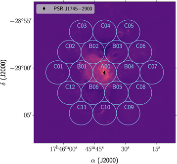
Figure 1. 4–8 GHz BL GC survey field comprised of 19 distinct pointings (light blue circles) of θHPBW ≈ 25 each. The background image is a 5.5 GHz Jansky Very Large Array continuum image (Zhao et al. 2016) of the Sgr A* complex. The GC magnetar PSR J1745−2900 (black diamond) is contained in our central pointing A00. All known pulsars lie ≳10′ away from Sgr A*, i.e., outside of our survey footprint.
Download figure:
Standard image High-resolution imageTable 1 presents an overview of our 4–8 GHz observations 10 distributed across four epochs during 2019 August–September. Our observing program consists of eleven deep integrations (≥30 minutes) on A00, two 5 minute scans on C10, and three 5 minute cadences on each of the remaining pointings. In addition, we observed test pulsars at three epochs, and confirmed their respective detections to verify our system integrity. To identify and reject radio frequency interference (RFI) via position switching, we conducted alternating observations of pairs of pointings in rings B and C. Pointing pairs were chosen such that the beam centers of grouped pointings were separated by at least 2θHPBW on the sky.
Table 1. Log of 4–8 GHz GBT Observations Analyzed in our Study
| Epoch | Start Date | Start MJD | Test Pulsars | Pointings | Nscans a | Scan Duration |
|---|---|---|---|---|---|---|
| (number) | (UTC) | (UTC) | (minutes) | |||
| 1 | 2019 Aug 7 | 58702.217 | B0355+54, J17441134 | (C01, C07) | (3, 2) | 5 |
| 2 | 2019 Aug 9 | 58704.993 | B1133+16, J17441134 | C07 | 1 | 5 |
| (B01, B04) | (3, 3) | 5 | ||||
| (B02, B05) | (3, 3) | 5 | ||||
| (B03, B06) | (3, 3) | 5 | ||||
| (C02, C04) | (3, 3) | 5 | ||||
| (C03, C05) | (3, 3) | 5 | ||||
| (C06, C08) | (3, 3) | 5 | ||||
| (C09, C11) | (3, 3) | 5 | ||||
| (C10, C12) | (2, 3) | 5 | ||||
| A00 | 1 | 60 | ||||
| 3 | 2019 Sep 8 | 58734.958 | ⋯ | A00 | 2 | 30 |
| 4 b | 2019 Sep 11 | 58737.962 | B2021+51 | A00 | 8 | 30 |
a Number of scans per pointing. For a pointing pair (X, Y), (NX , NY ) denotes the number of scans of X and Y, respectively. b Epoch 4 included position-switched observations of the flux density calibrator 3C 286.
Download table as: ASCIITypeset image
To accommodate various science cases, baseband voltages gathered during our observations were channelized to different spectral and temporal resolutions using the Breakthrough Listen Digital Backend (MacMahon et al. 2018; Lebofsky et al. 2019). Here, for our pulsar searches, we worked with total intensity filterbank data (no coherent dedispersion performed) having ≈43.69 μs time sampling and ≈91.67 kHz channel bandwidth. These data contain 53,248 channels spanning 3.56–8.44 GHz, which covers the 3.9–8.0 GHz instantaneous response of the C-band receiver.
2.1. Data Preprocessing
We followed the methodology of Suresh et al. (2021) to excise RFI from our data using the rfifind module of the pulsar software package PRESTO (Ransom 2011). Adopting an integration time of 1 s for our rfifind runs, we detected bright, persistent interference between 4.24–4.39, 4.90–4.95, and 6.90–7.10 GHz. Incorporating our rfifind mask and clipping bandpass edges, the usable radio frequency band in our data extends between 4.4 and 8.0 GHz.
After RFI masking, we dedispersed our dynamic spectra (radio frequency time data) at 1836 trial dispersion measures (DMs) between 0 pc cm−3 and 5505 pc cm−3 (both limits included) with a grid spacing of 3 pc cm−3. These dedispersed data were summed over the entire usable band, and then block-averaged by a factor of 8 to output dedispersed time series with a sample interval, tsamp ≈ 349.53 μs.
2.2. Red Noise Removal
Slow pulsar discovery (P0 ≥ 1 s) in long time series (T ≥ 5 minutes) often suffers from the presence of low-frequency noise in Fourier-domain spectra. To alleviate the adverse impact of red noise on our pulsar searches, we detrended our dedispersed time series using a running median window of width Wmed.
For deciding on an optimal value of Wmed, we visually inspected the effect of different trial Wmed on power spectra of barycentric GC magnetar time series (DM = 1776 pc cm−3,  ; Suresh et al. 2021). Starting at Wmed = 4 s, we successively lowered Wmed by factors of 2 until a further reduction in Wmed brought no concomitant increase in the number of harmonics of f0
mag seen in the power spectrum. In doing so, we settled at Wmed = 0.25 s for removing slow baseline fluctuations in our dedispersed time series.
; Suresh et al. 2021). Starting at Wmed = 4 s, we successively lowered Wmed by factors of 2 until a further reduction in Wmed brought no concomitant increase in the number of harmonics of f0
mag seen in the power spectrum. In doing so, we settled at Wmed = 0.25 s for removing slow baseline fluctuations in our dedispersed time series.
Figure 2 shows the result of time series detrending on the power spectrum of a barycentric DM = 1776 pc cm−3 time series from a 30 minute A00 scan. The power spectrum of the detrended time series evidently reveals significant peaks at f0 mag and its first seven harmonics. Without detrending, these peaks remain buried within red noise in the power spectrum of the original time series.
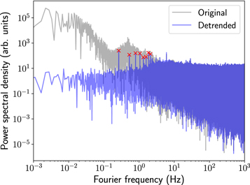
Figure 2. Power spectra of barycentric DM = 1776 pc cm−3 time series from a 30 minute A00 scan before (gray) and after (blue) detrending with a running median filter of width 0.25 s. The red crosses label the fundamental rotation frequency of the GC magnetar and its harmonics. The red noise in the gray power spectrum below 4 Hz arises from gradual baseline fluctuations in our original time series.
Download figure:
Standard image High-resolution imageFinally, to limit the false-positive count in our pulsar searches, we masked periodic RFI in the power spectra of our detrended time series. Looking at power spectra of topocentric DM = 0 pc cm−3 time series, we identified and flagged significant spikes at frequencies of 1.2, 6, and 60 Hz (US electric power line frequency), and their first five harmonics. The resulting cleaned power spectra constituted the basis of our Fourier-domain periodicity searches.
3. Periodicity Searches
Consider a regular pulse train (insignificant pulse jitter) from an isolated pulsar of barycentric rotational frequency, f0 = 1/P0. For an effective pulse duty cycle δeff, the energy in the pulse train gets distributed over Nh ≃1/2δeff independent harmonics in the power spectrum. Consequently, standard periodicity searches perform harmonic summing in power spectra of dedispersed time series to increase the significance of a pulsar detection (Ransom et al. 2002). In a blind search, the pulsar DM, f0, and δeff are unknown apriori. Searches for isolated pulsars, hence require sampling of the three-dimensional parameter space DM–f–Nh .
Binary orbital motion complicates pulsar detection by introducing a time-dependent Doppler drift that smears harmonics in the power spectrum. Conventional search algorithms attempt to retroactively correct for this smearing by presuming a constant or linearly evolving line-of-sight pulsar acceleration (Ransom et al. 2002; Andersen & Ransom 2018).
Figure 3 shows a binary pulsar orbit and its Keplerian orbital elements, including its projected semimajor axis ap = a sin i (orbital semimajor axis a and inclination i), argument of periapsis ω, and true anomaly AT . In the Newtonian regime, the line-of-sight pulsar acceleration (al ) and jerk (jl ) are respectively given by Bagchi et al. (2013); Liu et al. (2021):
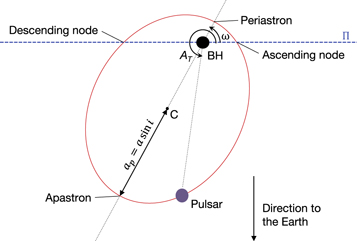
Figure 3. A pulsar orbiting a black hole. The pulsar orbit (red ellipse) has been projected onto a plane containing the direction to the Earth and the line Π connecting the two nodes. The symbols a, i, ω, and AT represent, respectively, the orbital semimajor axis, the orbital inclination, the argument of periapsis, and the pulsar true anomaly. The quantity ap = a sin i is the projected semimajor axis of the pulsar orbit centered at C.
Download figure:
Standard image High-resolution imageIn the above equations, e denotes the eccentricity of the pulsar orbit. Casting al and jl in dimensionless units, and introducing the harmonic number h, we have


Here, h = 1 labels the fundamental frequency f, and c is the vacuum speed of light. Following Andersen & Ransom (2018), we define the dimensionless Fourier frequency, r = fT. The quantities z and w thus represent the number of bins of signal drift in r and  over time T. In Equations (3) and (4), we note that both z and w scale linearly with h. Therefore, orbital motion lowers the detection significance of all harmonics in the power spectrum, with greater deleterious effects for higher harmonics. The most minimal regime of pulsar detection then occurs when only the fundamental survives with adequate significance in the power spectrum, while all higher harmonics have been smeared into the continuum by orbital motion.
3.1. Acceleration and Jerk Searches
The accelsearch routine of PRESTO (Ransom 2011) executes a matched filtering scheme that accounts for Fourier-domain power smearing of the highest harmonic up to a Fourier acceleration zmax and a Fourier jerk wmax (Ransom et al. 2002; Andersen & Ransom 2018). Searches for binary pulsars, hence involve sampling over five parameters, i.e., the DM, f, Nh , zmax, and wmax.
We targeted the discovery of pulsars in compact orbits around Sgr A* or stellar-mass BHs. We focused our searches on CPs as we expected most MSPs to fall below our detection threshold (see Section 4). To identify suitable trial parameter values for our binary pulsar searches, we considered a Mp = 2.14 M⊙ pulsar (highest neutron star mass measured to date; Cromartie et al. 2020) located at AT = −90°in an edge-on orbit (i = 90°) with ω = 0°. We further envisaged Nh = 1 searches for pulsars in tight binaries with large al and jl .
Assuming T = 30 minutes and P0 = 1 s, Figure 4 shows contours of constant wmax (top row) and zmax (middle row) for pulsar orbits around Sgr A* (left column) and a MBH = 9 M⊙ BH (median BH mass for solar metallicity; Woosley et al. 2020). The condition T ≲ 0.15Pb
for jerk searches restricts us to Pb
≳ 3.3 hr for T = 30 minutes. Setting Pb
= 10 hr as our target, we sought to cover ![$e\in \left[0.0,0.8\right]$](https://content.cld.iop.org/journals/0004-637X/933/2/121/revision1/apjac74c0ieqn4.gif) by uniformly sampling the wmax versus zmax curves shown in the bottom row of Figure 4. For our selected MBH value, ap
varies inappreciably for known ranges of Mp
. Therefore, our chosen (zmax, wmax) tuples encompass all known pulsar masses, including the typical mass of 1.4 M⊙ (Zhang et al. 2011).
by uniformly sampling the wmax versus zmax curves shown in the bottom row of Figure 4. For our selected MBH value, ap
varies inappreciably for known ranges of Mp
. Therefore, our chosen (zmax, wmax) tuples encompass all known pulsar masses, including the typical mass of 1.4 M⊙ (Zhang et al. 2011).
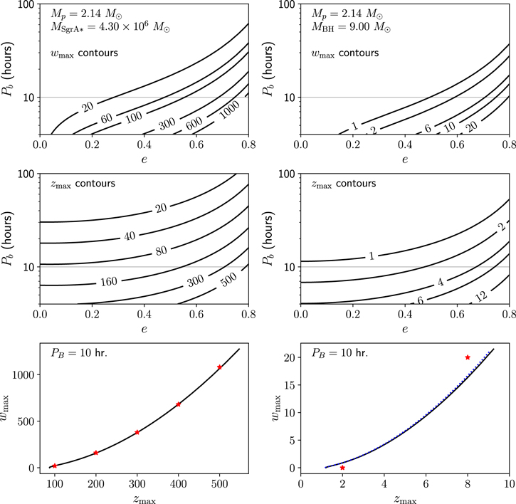
Figure 4. (zmax, wmax) curves for Nh = 1 binary pulsar searches. Top row: Contours of constant wmax for a 2.14 M⊙ pulsar orbiting Sgr A* (left column) and a 9 M⊙ BH (right column). Middle row: zmax contours for the same systems. Bottom row: wmax vs. zmax (black solid curves) for a binary orbital period of 10 hr, assuming a pulsar mass of 2.14 M⊙. While the black solid curve in the bottom left panel is insensitive to Mp , the blue dotted curve in the bottom right panel shows the corresponding trend for a 1.4 M⊙ pulsar orbiting a 9 M⊙ BH. The red stars mark (zmax, wmax) tuples chosen for our Fourier-domain jerk searches on T = 30 min. integrations. We note that the accelsearch module of PRESTO quantizes zmax and wmax in multiples of 2 and 20, respectively (Andersen & Ransom 2018). All panels assume P0 = 1 s, and edge-on pulsar orbits with ω = 0°and AT = −90°.
Download figure:
Standard image High-resolution imageTable 2 outlines our pulsar search strategy, wherein we also incorporated searches for isolated pulsars and binary pulsar orbits in the T = 5 minute integrations of our B- and C-ring pointings. Again, we identified viable zmax and wmax values considering Nh
= 1 searches for binary pulsar orbits. Adopting the same (zmax, wmax) tuples for our Nh
= {2, 4, 8} searches, we enhance our sensitivity to slowly orbiting pulsars through harmonic summing. However, since our searches perform matched filtering (Andersen & Ransom 2018) in the Fourier domain, the greatest sensitivity will be had for systems with al
= (zmax
c/Nh
f T2) and  .
.
Table 2. Pulsar Search Parameters
| Science targets | Pointings | Ta | Pb b | (zmax, wmax) |
|---|---|---|---|---|
| (minutes) | (hours) | |||
| Isolated pulsars | All | 5, 30, 60 | ⋯ | (0, 0) |
| Pulsars orbiting stellar-mass BHs | B-ring, C-ring | 5 | 1 | (2, 0), (6, 20) |
| A00 | 30 | 10 | (2, 0), (8, 20) | |
| Pulsars around Sgr A* | A00 | 30 | 10 | (100, 20), (200, 160), |
| (300, 380), (400, 680), | ||||
| (500, 1080) | ||||
Notes.
1. 1836 trial DMs explored between 0–5505 pc cm−3 (both limits included) with a grid spacing of 3 pc cm−3.
2. For a sample interval of ≈349.53 μs in the dedispersed time series, the range of f searched is 0–1430 Hz with a resolution of 1/T.
3. Trial Nh values considered = {1, 2, 4, 8}.
a Integration time. b Target binary orbital period assumed for specified (zmax, wmax) tuples.Download table as: ASCIITypeset image
Our pulsar search procedure on data can be described in three independent stages. First, we ran nonaccelerated searches for isolated pulsars on a per-scan basis. Second, at the trial parameter values listed in Table 2, we conducted acceleration and jerk searches on data from our 5 minute and 30 minute scans. Finally, we split our 60 minute A00 scan from epoch 2 into two contiguous halves, and executed jerk searches separately on each half.
Imposing a 6σps detection probability threshold in harmonic-summed power spectra, we used the accel_sift.py script of PRESTO (Ransom 2011) to group hits across adjacent trial DMs and frequencies f into distinct candidates. Here, σps measures the equivalent Gaussian significance of a frequency f in the χ2-distributed power spectrum (assuming Gaussian white noise background in detrended time series).
3.2. Results
Our pulsar searches yielded a total of 16,048 periodicity candidates across 64 scans. Table 3 presents our candidate detection statistics organized by pointings. Since we expect any astrophysical signal of our interest to be localized on the sky, we pruned our detection list by rejecting candidates common to paired pointings within a frequency tolerance Δf and a DM tolerance ΔDM. For an integration time T, we chose Δf = 1/2T, i.e., the maximum error on f for Nh = 1. Given an effective pulse width Weff = δeff P, the DM uncertainty associated with pulse detection across a usable bandwidth B is (Cordes & McLaughlin 2003)

Here, B ≈3.35 GHz, and νc ≈ 6.1 GHz is the center frequency of our observations. Conservatively setting Weff = 3tsamp ≈ 1 ms, we obtain ΔDM ≈ 33 pc cm−3. As evident from Table 3, our position-switched observations permit us to eliminate about 5% of candidates in rings B and C, thereby leaving us with 15,560 periodicity detections across 64 scans.
Table 3. Periodicity Detection Statistics
| Pointing | Ndetected a | Nrejected b | Ncands c |
|---|---|---|---|
| A00 | 7039 | ⋯ | 7039 |
| B01 | 454 | 27 | 427 |
| B02 | 487 | 22 | 465 |
| B03 | 495 | 26 | 469 |
| B04 | 460 | 34 | 426 |
| B05 | 414 | 25 | 389 |
| B06 | 485 | 25 | 460 |
| C01 | 481 | 13 | 468 |
| C02 | 456 | 27 | 429 |
| C03 | 489 | 36 | 453 |
| C04 | 437 | 25 | 412 |
| C05 | 554 | 28 | 526 |
| C06 | 596 | 48 | 548 |
| C07 | 458 | 12 | 446 |
| C08 | 423 | 33 | 390 |
| C09 | 555 | 46 | 509 |
| C10 | 370 | 12 | 358 |
| C11 | 413 | 38 | 375 |
| C12 | 982 | 11 | 971 |
| Total | 16048 | 488 | 15560 |
Notes.
a Number of distinct candidates detected at or above 6σps equivalent Gaussian significance in χ2-distributed power spectra. b Number of candidates rejected via position switching. c Number of candidates that pass comparisons between periodicity detections in paired pointings.Download table as: ASCIITypeset image
In Figures 5 and 6, we statistically analyze the remaining 15,560 candidates in terms of their DM, period (P = 1/f), and σps distributions. The GC magnetar markedly stands out as a high significance cluster of A00 candidates centered at DM = 1776 pc cm−3 and P = 3.7686 s. Furthermore, nearly 90% of candidates fall within a horizontal expanse between P = 2 ms and P = 100 ms in the P–DM plane. We attribute this scatter of candidates partly to a statistical sampling effect (greater number of power spectrum samples across P ∈ [2, 100] ms than that spanning P ∈ [102, 104] ms), and partly to noise and intermittent band-limited periodic RFI in dynamic spectra. Appendix A shows the average profiles of two sample candidates, whose phase-resolved dynamic spectra reveal bright RFI between 4.4–4.9, 5.1–5.2, 6.8–7.0, and 7.5–7.8 GHz. These narrowband structures asynchronously wax and wane during our observations, leading to a horde of nonastrophysical candidates detected at numerous DMs and periods.
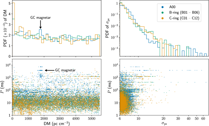
Figure 5. Top left panel: probability distribution function (PDF) of candidate DMs binned uniformly to 141 pc cm−3 resolution. Top right panel: PDF of equivalent Gaussian significance (σps) of candidates in power spectra. Plotted bins are linear in ln σps with width ≈0.06. Bottom left panel: Scatter of candidates in the period–DM plane. Bottom right panel: period–σps scatter of candidates. In all panels, the blue, green, and orange colors represent A00, B-ring, and C-ring, respectively.
Download figure:
Standard image High-resolution image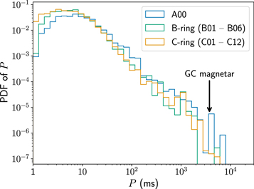
Figure 6. PDF of candidate periods (P) organized by rings. Histogram bins are evenly spaced in ln P with width ≈0.26 s.
Download figure:
Standard image High-resolution imageOther notable features in Figure 5 include streaks of A00 candidates at P ∈ [30, 100] ms, and an excess of C-ring candidates at P ≲ 2 ms and DM ∈ [0, 150] ∪ [430, 700] ∪ [1000, 1150] pc cm−3. Upon manual visual inspection of their respective folded profiles, we traced the A00 streaks to periodic irregularities occurring near the start and end of individual scans. Further, we associate the surfeit of C-ring candidates with the emergence of bright RFI at 5.8–5.9 and 7.8–7.9 GHz during our C12 scans.
In summary, we report the successful detection of the GC magnetar in periodicity searches of our A00 scans. Setting a 6σps detection threshold for our Fourier-domain searches, we find no statistical evidence of novel periodic astrophysical emissions in the 4–8 GHz BL GC survey data.
4. Survey Sensitivity Estimation
Consider the minimal detection of a pulsar, with only its h = 1 harmonic visible in the power spectrum. In such a circumstance, the relevant theoretical detection limit is the single harmonic sensitivity at f0 given by

Here, Ssys is the system-equivalent flux density (SEFD), and m = 6 is the minimum significance required to claim a detection. Often, Ssys in GC surveys is written as a sum of two terms.

where Ssys off − SgrA* is the SEFD away from the Sgr A* complex, and Ssys SgrA* captures the SEFD contribution from the Sgr A* complex.
Assuming slow pulsar orbital motion in time T, we can lower our sensitivity threshold below Ssh by summing over harmonics in the power spectrum. For δeff ≪ 1, the corresponding minimum detectable flux density (Dewey et al. 1985) is then

Appendix B describes various sources of pulse broadening that can widen a pulse from intrinsic width Wint to effective width, Weff = δeff P in a dedispersed time series. We define δint = Wint/P as the intrinsic pulse duty cycle. From the ATNF pulsar catalog v1.66 (Manchester et al. 2001) 11 , about 83% of CPs have duty cycles between 1% and 10%, with a median duty cycle of 2.5%.
Assuming negligible instrumental and dispersive pulse broadening,

Here, τsc(ν) is the scatter-broadening timescale. In the absence of alternate observational evidence, we take τsc toward the GC magnetar to be representative of the central ISM throughout the remainder of our study. From Spitler et al. (2014), we have

for GC magnetar pulses. Thus, scattering inhibits the detection of GC pulsars with P0 ≤ τsc(6.1 GHz) ≃1.35 ms.
Table 4 lists observational parameters and theoretical sensitivity limits of GC pulsar surveys conducted at νc
between 4–9 GHz. We adopted a GC distance, dGC = 8.18 kpc (Gravity Collaboration et al. 2019), to convert Ssh and Smin to pseudo luminosities, Lsh and Lmin, respectively. To facilitate sensitivity comparison across surveys at different νc
, we scaled their respective Lmin to 6.1 GHz invoking  , where α = −1.4 is the mean pulsar spectral index (Bates et al. 2013). This scaling preserves the fraction of known pulsars with spectral pseudo luminosity,
  for a given survey.
Table 4. Observing Parameters and Sensitivity Thresholds for GC Pulsar Surveys Conducted at 4–9 GHz
| Survey | νc | B | T | tsamp | Ssys (νc ) a | Lsh (νc ) b | Lmin (νc ) c | Lmin (6.1 GHz) d |
|---|---|---|---|---|---|---|---|---|
| (GHz) | (GHz) | (min.) | (ms) | (Jy) | (mJy kpc2) | (mJy kpc2) | (mJy kpc2) | |
| Johnston et al. (2006) | 8.4 | 0.864 | 70 | 1.0 | 148 | 22.1 | 3.5 | 5.5 |
| Deneva et al. (2009) | 4.8 | 0.8 | 60 | 0.65 | 57.5 e | 9.6 | 1.5 | 1.1 |
| Bates et al. (2011) | 6.59 | 0.576 | 280 | 0.13 | 216.7 | 19.8 | 3.2 | 3.5 |
| Eatough et al. (2021) | 4.85 | 0.5 | 72 | 0.26 | 129 | 24.9 | 4.0 | 2.9 |
| 8.35 | 0.5 | 144 | 0.13 | 93.3 | 12.7 | 2.0 | 3.2 | |
| This work f : | ||||||||
| A00 | 6.1 | 3.35 | 30 | 0.35 | 46.3 | 5.3 | 0.9 | 0.9 |
| Off-Sgr A* pointings g | 6.1 | 3.35 | 5 | 0.35 | 10.7 | 3.0 | 0.5 | 0.5 |
Notes.
a .
b
Single harmonic pseudo-luminosity threshold, Lsh = Ssh
dGC
2, where dGC = 8.18 kpc (Gravity Collaboration et al. 2019).
c
Minimum detectable pseudo luminosity, Lmin (νc
) = Smin (νc
) dGC
2 for δint = 2.5% and P0 = 1 s.
d
.
b
Single harmonic pseudo-luminosity threshold, Lsh = Ssh
dGC
2, where dGC = 8.18 kpc (Gravity Collaboration et al. 2019).
c
Minimum detectable pseudo luminosity, Lmin (νc
) = Smin (νc
) dGC
2 for δint = 2.5% and P0 = 1 s.
d
 invoked, where α = −1.4 is the mean pulsar spectral index (Bates et al. 2013).
e
TGC(ν) ≈ 568 K (ν/1 GHz)−1.13 (Rajwade et al. 2017) assumed to compute Ssys
SgrA*.
f
We estimated Ssys
off − GC and Ssys
SgrA* using Figure 1 and Equation (2) of Suresh et al. (2021).
g
B-ring and C-ring pointings with negligible Ssys
SgrA* in Figure 1.
invoked, where α = −1.4 is the mean pulsar spectral index (Bates et al. 2013).
e
TGC(ν) ≈ 568 K (ν/1 GHz)−1.13 (Rajwade et al. 2017) assumed to compute Ssys
SgrA*.
f
We estimated Ssys
off − GC and Ssys
SgrA* using Figure 1 and Equation (2) of Suresh et al. (2021).
g
B-ring and C-ring pointings with negligible Ssys
SgrA* in Figure 1.Download table as: ASCIITypeset image
Applying the above power-law scaling and assuming δint = 2.5%, Figure 7 shows Lmin(6.1 GHz) for various surveys as a function of P0. Our survey clearly represents the most sensitive 4–8 GHz exploration for GC pulsars conducted to date. For P0 ≳ 100 ms, our survey reaches down to Lmin ≈ 0.9 mJy kpc2, i.e., an 18% improvement over Deneva et al. (2009), who also utilized the GBT for their observations. However, at νc = 4.8 GHz, scattering limits the Deneva et al. (2009) sensitivity for P0 ≲ 100 ms, with P0 ≤ 3.4 ms pulsars rendered undetectable. In contrast, our survey still provides significant sensitivity to P0 ≥ 1.35 ms, thereby extending our discovery phase space to include potential superluminous MSPs (L6.1 ≥ 6 mJy kpc2, P0 ≈ 3 ms) residing at the GC.
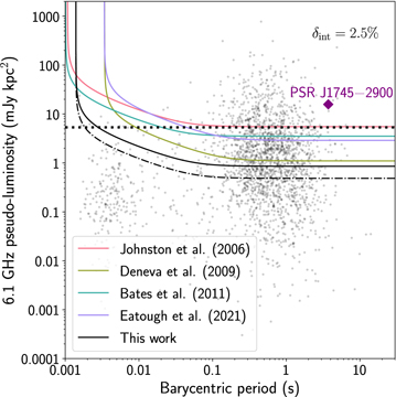
Figure 7. Lmin (6.1 GHz) curves for different GC pulsar surveys (various colors). The solid curves represent Lmin (6.1 GHz) for GC pointings at the survey parameters listed in Table 4. For Eatough et al. (2021), the plotted curve corresponds to their 4.85 GHz observations. The dashed–dotted black curves indicate Lmin for our T = 5 minute pointings away from the Sgr A* complex. All curves assume δint = 2.5% (median duty cycle for CPs). The black dotted line marks the single harmonic sensitivity for our T = 30 minutes GC scans. The background shows a scatter of 2197 pulsars with known 1.4 GHz flux densities (S1.4) and known distances in the ATNF pulsar catalog v1.66. We scaled S1.4 to 6.1 GHz assuming Sν ∝ να , where α = − 1.4 is the mean pulsar spectral index (Bates et al. 2013). The GC magnetar PSR J1745−2900 is highlighted with a purple diamond marker.
Download figure:
Standard image High-resolution image4.1. Fake Pulsar Injection and Recovery
Equations (6) and (8) describe our survey sensitivity presuming ideal Gaussian, white noise backgrounds in dedispersed time series. However, real-world data frequently contains RFI and red noise, the latter of which substantially worsens our sensitivity to long P0 (Lazarus et al. 2015; van Heerden et al. 2017). Therefore, to measure our true survey sensitivity, we injected fake pulsars into our original dedispersed time series and verified their recovery.
Following Section 2.2 of Suresh et al. (2021), we first calibrated 11,016 dedispersed time series from six 30 minute A00 scans at epoch 4 (MJD 58738). To simulate a fake pulsar, we began with an input δint, P0, and a 6.1 GHz pseudo luminosity L6.1. We chose an initial pulse phase randomly from a standard uniform distribution. We then randomly drew Gaussian single pulse amplitudes  and FWHMs W from lognormal distributions with means (L6.1/ δint
dGC
2) and δint
P0 respectively. For both distributions, we assumed standard deviations equal to 5% of their respective means. To each W sample, we then added tsamp in quadrature. Utilizing the drawn
and FWHMs W from lognormal distributions with means (L6.1/ δint
dGC
2) and δint
P0 respectively. For both distributions, we assumed standard deviations equal to 5% of their respective means. To each W sample, we then added tsamp in quadrature. Utilizing the drawn  and updated W samples, we thus generated a periodic Gaussian pulse train that models a discretely sampled signal at the location of a pulsar (pulse jitter neglected). We next incorporated scattering by convolving the simulated Gaussian pulse train with a one-sided, decaying exponential of timescale, τsc(6.1 GHz) ≃1.35 ms. Finally, we added the resulting periodic signal to all calibrated time series to complete our fake pulsar injection. In the above exercise, we ignored instrumental and dispersive pulse broadening as these effects are negligible for the parameters of our survey and data processing (see Appendix B).
For every trial δint and P0, we kicked off our pulsar injections at L6.1 = 0.8Lmin. Passing all calibrated time series containing the injected signal through our processing pipeline (including time series detrending), we stepped up L6.1 in small increments until the detection significance of the artificial pulsar exceeded 6σps. Let Lmin true denote the minimum recovered L6.1 for a given trial δint and P0. Averaging Lmin true over identical fake pulsar injections in 11,016 calibrated time series, we obtained the dotted sensitivity curves shown in Figure 8.
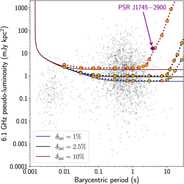
Figure 8. Theoretical (solid curves) and true sensitivity estimates (dotted curves) for different δint (various colors). All curves assume the survey parameters of our 30 minute A00 scans mentioned in Table 4. The duty cycles δint = 1% (dark blue) and δint = 10% (maroon) represent, respectively, the 10th and 93rd percentile of the empirical duty cycle distribution of CPs. The median δint of the corresponding distribution is 2.5% (black). The orange circular markers indicate minimum recovered 6.1 GHz pseudo-luminosities of fake pulsar injections at different trials δint and P0. As in Figure 7, the background plot is a scatter of 2197 pulsars from the ATNF pulsar catalog v1.66. The GC magnetar PSR J1745−2900 is labeled with a purple diamond marker.
Download figure:
Standard image High-resolution imageNoticeably, RFI raises our survey sensitivity above theoretical limits by 3%–7% across all P0. Moreover, the presence of red noise in our raw data progressively hinders our search sensitivity at longer P0 and larger δint. However, despite the deleterious impact of red noise and RFI on our pulsar searches, our survey crucially retains adequate sensitivity to over 95% of theoretically detectable pulsars for a median CP δint of 2.5%.
5. Summary and Discussion
We have conducted a comprehensive 4–8 GHz search of the central 625 (≈14.9 pc in projection) of our galaxy for pulsars. Utilizing the GBT, our observing program comprised of 11 T ≥ 30 minutes integrations on the GC and 53 T = 5 minutes integrations on nearby Galactic bulge fields. As proof of our survey integrity, we successfully demonstrated the detection of the GC magnetar PSR J1745−2900 in all of our GC scans. Executing Fourier-domain acceleration and jerk searches, we report the nondetection of hitherto unknown periodic astrophysical emissions in our data above a 6σ detection threshold.
Our investigations constitute the most sensitive 4–8 GHz exploration for GC pulsars conducted to date. For δint = 2.5% and P0 ≃ 1 s, our survey reaches down to Lmin true ≈ 1 mJy kpc2, i.e., a sensitivity improvement of at least 18% over past GC pulsar searches conducted at similar radio frequencies. Notably, our observations open the window to discovering potential superluminous MSPs (L6.1 ≥ 6 mJy kpc2, P0 ≈ 3 ms) at the GC. Though we focused our binary pulsar searches on CP orbits around Sgr A* or stellar-mass BHs, our chosen processing parameters in Table 2 also incorporate searches for bright MSPs with low radial pulsar accelerations (zmax ≲ 0.5P0, ms −1) and jerks (wmax ≲ 1.1P0, ms −1).
Studying pulsar demographics in our galaxy, Freire (2013) argued that the globular cluster pulsar population is likely older than its Galactic field counterpart. Analogous to globular clusters, the GC environment, with its high density of ∼106 stars per cubic parsec (Schödel et al. 2018), is predicted to favor MSP production. About 3% of Galactic field MSPs have the L6.1 ≥ Lmin true of our survey. Say that GC MSPs follow similar population-level statistics as their Galactic field equivalents. For a beaming fraction fb = 0.7 (Kramer et al. 1998), our nondetection of GC pulsars therefore constrains the total MSP count in the central parsec of our galaxy to NMSP ≲ 50. Our NMSP estimate is a factor of 20 smaller than that derived by Wharton et al. (2012), possibly due to our lack of sensitivity to tight MSP orbits. Sideband searches (Ransom et al. 2003) and coherent full-orbit demodulation algorithms (Allen et al. 2013; Balakrishnan et al. 2022) will both provide enhanced sensitivity to short binary orbital periods (Pb ≪ T), thereby yielding stronger constraints on the GC MSP population in the near future.
Alternatively, our nondetection of GC pulsars can be attributed to complex pulsar orbital dynamics arising from plausible close encounters with other neutron stars, stellar-mass BHs, and intermediate-mass BHs in the dense GC environment. Such proximate compact object flybys can potentially disrupt binaries and scatter pulsars into hyperbolic orbits that lead away from the GC (Jiale et al. 2021). On the other hand, a preference for magnetar formation (Dexter & O’Leary 2014) at the GC may explain the “missing pulsar problem” by virtue of the comparatively shorter magnetar lifetimes (∼104 yr).
Throughout our study, we presumed that interstellar scattering does not limit GC pulsar surveys. While τsc(ν) measurements of the GC magnetar support the above premise, observations of pulse broadening along different lines of sight are necessary to build a more complete picture of the turbulent central ISM. Hence, we encourage regular monitoring of the GC for fast transients to obtain robust scattering constraints on the ionized central ISM, and thus better inform future GC pulsar surveys.
A.S. thanks Scott M. Ransom for timely responses to software-related queries. A.S., J.M.C., and S.C. acknowledge support from the National Science Foundation (AAG 1815242). J.M.C. and S.C. are members of the NANOGrav Physics Frontiers Center, which is supported by the NSF award PHY–1430284. Breakthrough Listen is managed by the Breakthrough Initiatives, sponsored by the Breakthrough Prize Foundation. The Green Bank Observatory is a facility of the National Science Foundation, operated under a cooperative agreement by Associated Universities, Inc.
This work used the Extreme Science and Engineering Discovery Environment (XSEDE) through allocations PHY200054 and PHY210038, which are supported by the National Science Foundation grant number ACI−1548562. Specifically, it used the Bridges-2 system, which is supported by NSF award number ACI−1928147, at the Pittsburgh Supercomputing Center (PSC).
Facilities: GBT, XSEDE (Towns et al. 2014).
Software: Astropy (Astropy Collaboration et al. 2013, 2018), NumPy (van der Walt et al. 2011), Matplotlib (Hunter 2007), PRESTO (Ransom 2011), Python 3 (https://www.python.org), SciPy (Virtanen et al. 2020).
Appendix A: Pulse-Averaged Profiles of Sample Periodicity Candidates
Figures A1 and A2 show average profiles of two sample candidates that sit amidst the large scatter of detections between P = 2 ms and P = 100 ms in the P–DM plane of Figure 5. Average profiles were generated using the prepfold routine of PRESTO (Ransom 2011).
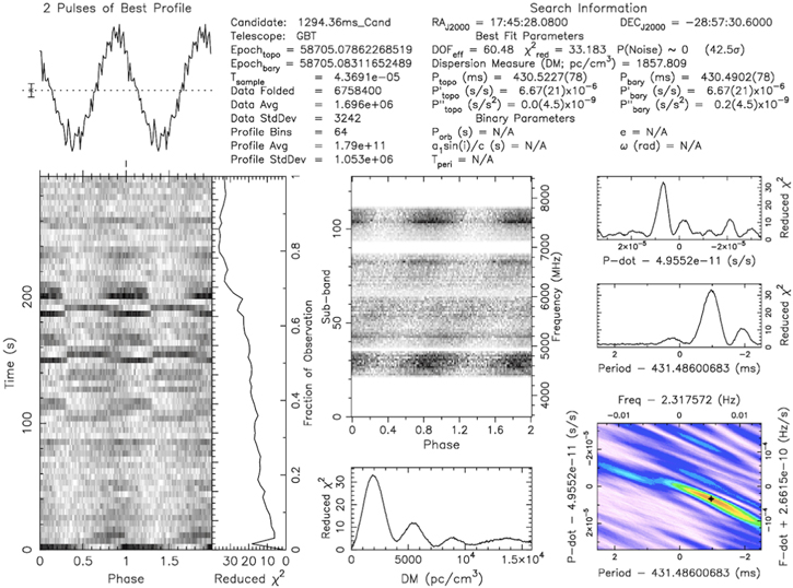
Figure A1. A sample periodicity detection in pointing C04 that falls within the sea of candidates between P = 2 ms and P = 100 ms in the P–DM plane (see Figure 5). Top left panel: average pulse profile of the candidate. Bottom left panel: rotation-resolved profile with flux density shown on the grayscale. The reduced χ2 measures the departure of the pulse-averaged profile from a flat noisy model. Top middle panel: phase-resolved dynamic spectrum of the candidate. Bottom middle panel: variation of the reduced χ2 with DM. Top right panel: reduced χ2 vs. period derivative  . Central right panel: reduced χ2 vs. folding period (P). Bottom right panel: raster plot of the reduced χ2 in the
  plane. The pulsation significance (42.5σ) quoted in the top right corner quantifies the equivalent Gaussian detection probability determined from the reduced χ2 of the average profile.
Download figure:
Standard image High-resolution image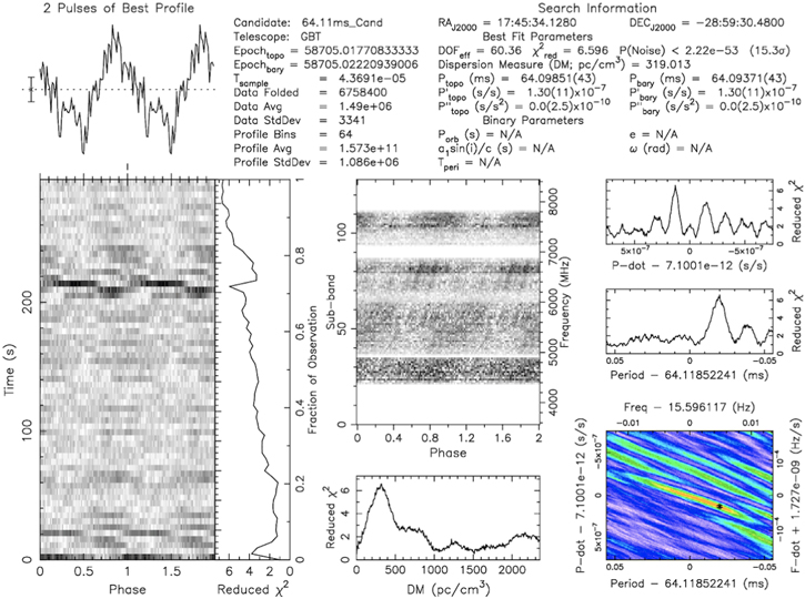
Figure A2. A prepfold output of a periodicity detection in pointing B02.
Download figure:
Standard image High-resolution imageAppendix B: Effective Single Pulse Widths in Dedispersed Time Series
Consider a pulsar emitting single pulses of average intrinsic width Wint. Accounting for instrumental effects, sampling, and propagation-induced broadening, the effective pulse width in a dedispersed time series is
Here, tsamp is the sample interval in the dedispersed time series, and tR ∼ (Δνch)−1 is the receiver filter response time for a channel bandwidth Δνch.
The term tchan represents the intrachannel dispersive smearing given by Cordes & McLaughlin (2003)

Further, tBW quantifies the residual broadband dispersive delay for a DM error ΔDM.
Finally, τsc(ν) is the pulse-broadening timescale from multipath wave propagation through turbulent ionized plasma.
For our observations, νc ≈ 6.1 GHz, B ≈ 3.35 GHz, Δνch ≈91.67 kHz, and tsamp ≈ 349.53 μs. Working with a DM step size of 3 pc cm−3, our trial DMs are at best ΔDM = 1.5 pc cm−3 off from the true DM of a source. Collectively, the above numbers imply tR ∼ 11 μs, tBW ≈ 184 μs, and tchan ≈ 6 μs for DM = 1776 pc cm−3 of the GC magnetar (Suresh et al. 2021). Assuming the empirical GC magnetar scattering law (Spitler et al. 2014) given in Equation 10, τsc ≃1.35 ms at 6.1 GHz.
Since τsc ≫ tchan, tBW, tR , Equation B1 can thus be simplified to

Footnotes
- 8
We define MSPs as pulsars with barycentric rotational periods, P0 < 30 ms.
- 9
We define CPs as pulsars with P0 ≥ 30 ms.
- 10
Links for data download: http://blpd9.ssl.berkeley.edu/GCrawspec/, http://blpd12.ssl.berkeley.edu/GCrawspec/.
- 11