Abstract
In a companion paper, we develop a theory for the evolution of stellar wind-driven bubbles in dense, turbulent clouds. This theory proposes that turbulent mixing at a fractal bubble/shell interface leads to highly efficient cooling, in which the vast majority of the input wind energy is radiated away. This energy loss renders the majority of the bubble evolution momentum driven rather than energy driven, with expansion velocities and pressures orders of magnitude lower than in the classical Weaver et al. solution. In this paper, we validate our theory with three-dimensional, hydrodynamic simulations. We show that extreme cooling is not only possible, but is generic to star formation in turbulent clouds over more than three orders of magnitude in density. We quantify the few free parameters in our theory, and show that the momentum exceeds the wind input rate by only a factor  . We verify that the bubble/cloud interface is a fractal with dimension
  . The measured turbulent amplitude (
 ) in the hot gas near the interface is shown to be consistent with theoretical requirements for turbulent diffusion to efficiently mix and radiate away most of the wind energy. The fraction of energy remaining after cooling is only
  , decreasing with time, explaining observations that indicate low hot-gas content and weak dynamical effects of stellar winds.
1. Introduction
Feedback from massive stars is thought to be the dominant process setting the lifetime efficiency of star formation on the scale of individual molecular clouds (Lada & Lada 2003; McKee & Ostriker 2007). Luminous hot stars use their strong radiation to disperse the surrounding dense gas in several ways: imparting primarily outward photon momentum to gas and dust where stellar UV/optical radiation is first absorbed (direct radiation pressure); imparting preferentially outward photon momentum to dust where diffuse infrared is absorbed (reprocessed radiation pressure); ionizing and heating gas, which leads to over-pressured expansion of ionized gas and creates a rocket effect on neutral structures where photoevaporation occurs (pressure of photoionized gas); or directly depositing momentum in the star’s own atmosphere, resulting in high-velocity stellar winds that shock and transfer momentum to the ambient gas. It is much debated in the literature which of these mechanisms dominates in which situations within the star-forming interstellar medium (ISM) (Krumholz et al. 2019). While several recent efforts have used numerical radiation hydrodynamic simulations for in-depth studies of the effects of radiation feedback on star-forming clouds (Dale et al. 2012, 2013; Walch et al. 2012; Raskutti et al. 2016, 2017; Howard et al. 2017; Kim et al. 2018, 2019, 2021; Geen et al. 2020, 2021; Grudić et al. 2020; Fukushima et al. 2020), there have been fewer detailed numerical studies of stellar wind feedback (reviewed below). In this paper, we focus on the thermal and dynamical effects of stellar winds driven by star clusters in their natal molecular clouds.
In an accompanying paper (Lancaster et al. 2021, hereafter, Paper I) we have theoretically investigated the dynamics of expanding stellar wind bubbles in the case that most of the wind’s energy is radiated away. There, we argue that the interface between hot bubbles and the surrounding gas is subject to strong turbulent mixing, which subsequently leads to efficient radiative cooling in intermediate-temperature gas. We also argue that the surface of the hot bubble is a fractal, and the large associated area enhances cooling. We hypothesize that efficient cooling leads to the dominant phase of bubble evolution being momentum driven rather than energy driven. In this work, we support the theoretical model of Paper I with a suite of three-dimensional (3D) hydrodynamic simulations, which we analyze to provide quantitative corroboration of the arguments made there. Each simulation follows the expansion of a hot bubble driven into the surrounding dense, turbulent ISM by a constant luminosity point source.
Several numerical studies have previously explored the dynamical effects of main-sequence stellar winds on their environment. These have included one-dimensional numerical models (Garcia-Segura et al. 1996a, 1996b; Silich & Tenorio-Tagle 2013; Krause et al. 2016; Fierlinger et al. 2016; Rahner et al. 2017) some of which have incorporated phenomenological accounts of 3D processes such as energy leakage (Harper-Clark & Murray 2009) and turbulent diffusivity that leads to cooling (El-Badry et al. 2019). These problems have also been explored in two-dimensional studies, which have sought to examine filamentation at reduced computational expense (Freyer et al. 2003, 2006; Wünsch et al. 2008; Ntormousi et al. 2011; Dwarkadas & Rosenberg 2013). Finally, numerical investigations of stellar wind feedback effects in 3D have ranged from targeted studies of winds (Dale et al. 2013; Krause et al. 2013; Rogers & Pittard 2013; Krause & Diehl 2014; Offner & Arce 2015; Wareing et al. 2017; Dale & Bonnell 2008) to comparisons of winds and photoionization heating over a range of parameter space (Dale et al. 2014; Geen et al. 2015; Haid et al. 2018; Geen et al. 2021). These simulations have contributed to assessments of the relative contribution of winds in a number of scenarios and over a range of densities and cloud masses. Some have additionally tried to constrain the relative contribution of leakage and turbulent mixing.
In this paper, we explore a set of questions related to the detailed structure and evolution of bubbles driven by stellar winds in turbulent clouds. Our goals are to characterize the dependence of bubble evolution on input wind power and ambient cloud properties, and to explain the physical mechanisms controlling the evolution. Using numerical simulations, we quantify (1) the temporal evolution of wind bubble sizes and the energy and momentum that bubbles/shells contain; (2) the properties of the turbulence that drives mixing at the interface between a bubble’s hot/diffuse interior and cool/dense shell; (3) the fractal structure and foldedness of the cooling interface; and (4) the total energy losses to cooling due to turbulent mixing. Confirming the theory laid out in Paper I, we shall show that for the conditions within star-forming clouds, the vast majority of wind energy is expected to be lost due to turbulent mixing followed by radiative cooling, and that the large area associated with the fractal geometry of the bubble/cloud interface is crucial to enhancing losses. Our physical picture of turbulent, cooling mixing layers is much informed by insights from recent numerical and analytic investigations of the Kelvin–Helmholtz (KH) instability in the context of multiphase galactic winds and the circumgalactic medium (Gronke & Oh 2018; Fielding et al. 2020; Tan et al. 2021).
The numerical model we adopt is intentionally idealized. It is designed to provide a testing ground for the theory presented in Paper I that represents key real-world features (to the extent that is computationally practical), while still having that theory be applicable. To that end, we (i) have ignored the effects of star formation that is extended in both space and time, (ii) approximated the winds as having constant mechanical luminosity, (iii) ignored the effects of magnetic fields and stellar radiation, and (iv) adopted the assumption of collisional and ionization equilibrium for computing cooling losses in ionized gas, and a simple analytic fit for cooling in warm/cold neutral gas. Thus, our simulations are designed to test our theoretical predictions, rather than faithfully represent the real world. By tackling an idealized numerical problem, however, we are able to validate our theoretical framework and quantitative predictions that can be extrapolated beyond the necessarily limited scope of any single simulation suite.
The structure of this paper is as follows. In Section 2, we briefly review our theory for evolution of wind-driven bubbles. The reader is referred to Paper I for a complete description. In Section 3, we describe our numerical methods for implementing winds in the Athena code, as well as our simulation setup and the parameters of our model suite. We present the analysis of our results in Section 4 and conclude with a summary of our findings in Section 5.
2. Review of Paper I Theory: Wind Bubble Dynamics with Efficient Cooling
Our theory is developed in full in Paper I; for convenience we briefly summarize key features here. Our global dynamical evolution model is based on the premise that energy losses in the bubble/shell interface are so great that the bubble is effectively momentum driven rather than effectively energy driven. 1 We term this global solution the efficiently cooled (EC) stellar wind-driven bubble.
In the EC model, there is a point source of constant mechanical luminosity  and mass-loss rate
  , which injects into the surrounding cloud a wind with velocity

and momentum input rate

The momentum of the system is mostly contained in the bubble shell, and increases linearly in time as

This allows for amplification by a factor  (assumed order unity in the EC theory) above the value
  that corresponds to the momentum originally injected in the wind, which would apply if there is no thermal energy buildup within the bubble (maximally efficient mixing/cooling).
We define  as the radius of the sphere that has the same volume as the bubble:

Under the assumptions that the background density variations are statistically isotropic and homogeneous, and that the bubble’s momentum is given by Equation (3), the bubble’s effective radius evolves in time as

Here,  is another order-unity parameter that accounts for geometry;
  denotes the solution for an exactly spherical bubble expanding in a uniform ambient medium with momentum increasing at a rate
  . The scaling
  is shallower than
  for the classical energy-driven solution.
The total energy contained within the bubble interior is

where  quantifies the enhancement in energy above the case where the bubble is fully occupied by the free wind. For a spherically expanding bubble, we can write
  in terms of
  (see Equations (A13) and (A16) of Paper I), with
  within 6%.
The predicted pressure in the post-shock gas of the wind is
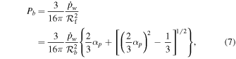
where  is the radius of the free wind region, defined analogously to Equation (4). From Equation (A14) of Paper I, the term in curly braces can be approximated as
  within 4% for
  .
.
The radial kinetic energy in the bubble’s shell is given by

The shell will also have turbulent motion, such that  is its total kinetic energy. We describe the level of turbulent energy relative to the radial kinetic energy as

Paper I shows that the above formulae can be combined to obtain a prediction for the fraction of input energy retained after cooling,

where  is the complementary fraction lost to cooling. To the extent that the terms in parentheses in Equation (10) are relatively constant, we would expect
  .
.
In Paper I, we hypothesize that the bubble/shell interface is a fractal. Under this assumption, the bubble’s total area when measured on scale ℓ becomes

where d is known as the excess fractal dimension of the surface and  is an order-unity parameter meant to account for any minor inconsistencies with this model.
Paper I argued that instabilities at the interface between the shocked wind and the surroundings drive turbulence that feeds off the kinetic energy in the shocked wind. The turbulence in the hot gas is assumed to follow a power-law form, such that  . Accounting for both the turbulent velocity and fractal area of the interface, the effective enthalpy flux at scale ℓ is then
  , where

defines an equivalent radial velocity through the turbulent mixing/cooling boundary layer for a bubble of size  . This enthalpy flux represents the capacity for mixing and radiative cooling, increasing to smaller scale until reaching the scale where
  , where

for Tpk the temperature of peak cooling. With pressure in the shocked gas given by Equation (7),  .
.
Finally, we note that Paper I outlined the conditions under which the EC regime should apply. One estimate, from comparing to the solution from El-Badry et al. (2019), gives an upper limit on the energy retention fraction for the EC solution to be valid:

Another limit is that the velocity of shocked hot gas flowing into the boundary layer,

cannot exceed the equivalent velocity that turbulent diffusion can accommodate, given in Equation (12).
3. Numerical Methods and Models
To test the theory presented in Paper I, we use the
Athena code (Stone et al. 2008) in running a series of 3D hydrodynamic simulations of constant luminosity stellar winds injected into turbulent clouds. We do not include any magnetic fields in the present simulations, but we do include cooling in the gas that is implemented as part of the Athena-TIGRESS code base for the star-forming multiphase ISM (Kim & Ostriker 2017, 2018). This implements cooling in an operator-split manner following Koyama & Inutsuka (2002) at  and Sutherland & Dopita (1993) at
  .
.
There is also uniform background heating of  , which decreases in hot, ionized gas; more details can be found in Section 2.3.1 of Kim & Ostriker (2017). All of our simulations are run using the linearized Roe Riemann solver (Roe 1981), second-order spatial reconstruction, and the unsplit van Leer integrator (Stone & Gardiner 2009).
3.1. Wind Injection
Here, we describe our treatment of stellar winds, which we implement in Athena in an operator-split fashion. We provide a quantitative test of this implementation in Appendix A. Each simulation contains a single wind source, which we refer to as a star particle, although in practice it represents a stellar cluster. This source particle is put in by hand and does not exert any gravitational force on the surrounding gas. Our approach employs a hybrid thermal/kinetic energy injection scheme that interpolates between pure thermal injection close to a source and pure kinetic injection toward the edge of the feedback region. There are multiple benefits to this hybrid energy injection approach. From a physical perspective, it more directly represents the reality of a bubble driven by a cluster of massive stars, wherein the majority of the energy close to the center of the bubble is thermal (due to shock thermalization through colliding winds of individual stars) while it is mostly kinetic toward the edges (where this thermal energy has managed to drive expansion). From a numerical perspective, for a purely kinetic feedback implementation the vector momentum field cannot be properly resolved immediately adjacent to the source. By transitioning to thermal energy injection near the source, it is only necessary to resolve a scalar field. An advantage of the hybrid approach over purely thermal energy injection is that the latter can require a larger spatial scale for pressure gradients to accelerate the flow modeling the primary wind.
Given a star particle at position  within the domain of the simulation, we deposit energy in the grid cells surrounding the star particle using a subcell method based on the implementation of Ressler et al. (2020). We specify
  , the radius of the spherical feedback region, and
  is the number of subcells per grid cell along a grid-aligned direction. When initializing the simulation we loop through a cube of
  subcells where

is the total number of subcells that could possibly lie within the feedback sphere along a grid-aligned direction and  denotes the ceiling function. The subcells within this cube are equally spaced along each grid-aligned direction between
  and
and  .
.
For each subcell in this cube with position  relative to the source, we determine if
  (i.e., if the subcell is within half a subcell spacing of the feedback radius or fully within the feedback radius) . If it is, we then record the position of the subcell
  for use within the full simulation. In order to account for the subcell volume only partially overlapping the actual feedback region, we additionally assign each subcell a weight
  according to
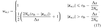
This formula is simply a linear interpolation between 1 and 0 over the radial range of ± half a subcell spacing from the feedback radius, which approximates the true volume fraction (Jones & Williams 2017). We additionally store the total effective volume that wind energy is injected into, defined as

Once the positions and weights of the subcell template are initialized, they are used for the hybrid thermal/kinetic energy injection.
Given a mechanical luminosity  and mass-loss rate
  for the wind, the mean mass density
  and energy density
  to be injected in a time
  are
are

For a given subcell in our template, indexed by i, we determine the grid cell in which it resides at location  , and increment the mass density by
  . For the purposes of the current paper,
  is always at the origin.
The total energy density in the target cell is similarly incremented by  . To compute the injected momentum, we specify the variable
  at a given subcell position
  according to

Once  is determined we define the injected momentum density as

As was noted in Wall et al. (2020), the presence of momentum and mass within the grid cell to which we are adding these quantities means that the kinetic energy added by the above change in momentum density is not
 , but actually somewhat less depending on what the initial density and momentum of the cell are. The discrepancy between the actual injected kinetic energy density and
  is especially important at the early times of wind onset, when the surrounding density is high, but becomes negligible once the wind has evacuated the feedback region. In the case where there is negligible preexisting energy and momentum, our prescription deposits 75% of the total energy as kinetic energy.
In order to make sure that our results are not affected by the details of our feedback mechanism, we run tests with  (purely thermal feedback) in Appendix B.1. This scenario might be closer to the truth of a cluster of stars whose colliding winds shock and turn initially kinetic energy into bulk thermal energy. We found that this pure thermal feedback scenario simply leads to a minor delay in the wind’s evolution, but broadly the results remain unchanged.
When we inject the wind mass into the feedback region, we add an equal amount of mass to a passive scalar variable, which is simply passively advected with the gas. We use this scalar to track the mixing of the wind material with the surrounding gas as well as a means of separating mass that has been swept up by the wind from the ambient medium, as we will explain in Section 4.
3.2. Model Parameters and Setup
Our goal is to span a large range of the potential parameter space for stellar winds originating from young star clusters within massive molecular clouds, which is where most star formation takes place. To that end, we consider three cloud masses  of 5 × 10⁴, 105, and
  , and four different cloud radii
  of 20, 10, 5, and 2.5 pc . The largest radii represent normal star-forming giant molecular cloud (GMCs), cases with intermediate radii may represent infrared dark clouds, and cases with the smallest radii may represent extremely dense cluster-forming clumps within larger GMCs or the natal clouds in which super star clusters are born in starbursting galactic centers.
Each choice of  and
and  corresponds to a choice of mean mass density
  as
as

where  is the mean molecular weight of the gas, mp
is the mass of a proton, and
is the mean molecular weight of the gas, mp
is the mass of a proton, and  is the mean number density of the hydrogen nuclei. Rather than creating spherical clouds within our cubic domain, we apply uniform density
  everywhere within a domain of side length
  . The global cloud parameters are just used for reference in setting the ambient conditions with which the wind interacts.
The grid has uniform spatial resolution in each dimension with Lbox/Δx = 128, 256, and 512 for the simulations with  and only Lbox/Δx = 128 and 256 for the simulations at higher and lower cloud mass. The parameters describing the simulation initial density conditions and numerical resolution are outlined in Table 1. Only the highest resolution is listed for each model.
Table 1. Parameters of Simulation Suite
| Cloud Mass | Cloud Radius |

|

|
 a
a
| Resolution a |
|---|---|---|---|---|---|

|

|

|

|

| |

| 20 | 43.1 | 3.59 | 0.15 | 2563 |

| 10 | 345 | 5.08 | 0.08 | 2563 |

| 5 | 2760 | 7.18 | 0.04 | 2563 |

| 2.5 | 22,800 | 10.2 | 0.02 | 2563 |
| 105 | 20 | 86.3 | 5.08 | 0.08 | 5123 |
| 105 | 10 | 690. | 7.18 | 0.04 | 5123 |
| 105 | 5 | 5520 | 10.2 | 0.02 | 5123 |
| 105 | 2.5 | 44,200 | 14.4 | 0.01 | 5123 |

| 20 | 431 | 11.4 | 0.15 | 2563 |

| 10 | 3450 | 16.1 | 0.08 | 2563 |

| 5 | 27,600 | 22.7 | 0.04 | 2563 |

| 2.5 | 228,000 | 32.1 | 0.02 | 2563 |
Notes. Each model is run with three different values for the mass of the wind source particle,  and 1.
Download table as: ASCIITypeset image
We initialize all the simulations at a uniform pressure of  . Since we evolve the simulations long enough for thermal relaxation to occur before initiating the wind, this particular choice of initial pressure is not important to our results. We also ran test simulations at a initial pressure of
  and found no differences.
Each simulation is initialized with a turbulent velocity field that is a Gaussian random field with power spectrum  for
for  . For higher resolution runs, the realization of the power spectrum uses a set of modes identical to those of the lower resolution case. The amplitude of the turbulence is chosen so that the initial kinetic energy per unit mass is equivalent to twice that of the gravitational potential for a sphere of radius
  and mass
  , i.e.,

where the tildes are used to indicate energy per unit mass. We note, however, that self-gravity is not included in the simulations.
For each simulation, we allow the turbulent velocity field to evolve and decay, without any additional driving, until the average kinetic energy per unit mass has decayed to  (i.e., it has been reduced by half). At the end of this initial evolution, each simulation has a turbulent velocity scale
  . For each model,
  is listed in Table 1.
At the same time as turbulence is decaying, the Reynolds stresses create an inhomogeneous density structure throughout the simulation domain. The turbulent decay period is generally one-tenth of the initial flow crossing time ( ) of the simulation domain, amounting to 0.03–0.7 Myr. Over this period, the thermal energy also relaxes, with temperature approaching thermal equilibrium; in the cold gas this is ∼30–200 K.
After the initial period of turbulent decay, we create a star particle at the center of the simulation domain of mass  . The parameter
  can be thought of as akin to a total star formation efficiency. For each set of initial conditions laid out in Table 1 we run simulations at
  and 1. The star particles inject energy and mass proportional to their own mass in accordance with the method described in Section 3.1, with a feedback radius
  at all resolutions, meaning that the feedback radius is resolved by a minimum of 3.2 resolution elements at the lowest resolution. We test this choice of feedback radius in Appendix B.3 and find it does not affect our results.
We adopt a constant wind luminosity per unit mass of  and mass-loss rate per unit mass
  . This mass-loss rate is about a factor of 5 larger than that expected for a standard solar metallicity population, with a Kroupa IMF (Kroupa 2001) as calculated by STARBURST99 (SB99; Leitherer et al. 1999). A comparison between the constant values that we adopt and those determined from SB99 is given in Figure 1. We use the larger mass-loss rate because this reduces the temperature of the shocked wind, yielding a less stringent time step.
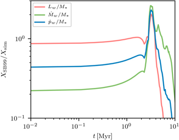
Figure 1. Ratio of the wind parameters derived using the population synthesis code SB99 to the constant values for each parameter that we adopt in our simulations.The SB99 mass-loss rate and momentum input rate are, respectively, a factor ∼5 and ∼2 lower than the ones we adopt. We validate that using the SB99 values does not change our conclusions (see Appendix B.2).
Download figure:
Standard image High-resolution imageOur adopted wind parameters correspond to a wind velocity of  and a momentum injection rate per unit of mass of
  . At the lower mass-loss rates consistent with the SB99 calculations, the wind velocity (momentum injection rate) is larger (smaller) by a factor
  , i.e.,
  and
and  . This only corresponds to a difference in radial evolution (according to our theory) of a factor of
  , so this should not affect the interpretation of our results. We have additionally run simulations with a standard mass-loss rate and have obtained consistent results, as described in Appendix B.2.
4. Numerical Results
Here, we lay out the results of the simulations described in Section 3.2. In our presentation, we shall focus on cases with  and use the remaining simulations for validation of the generality of our results, as summarized in Appendix C.
4.1. Cloud and Bubble Structure and Thermal Distributions
Example snapshots from our simulations are provided in Figure 2 ( and
and  model) and Figure 3 (
 and
and  model) in order to provide a more concrete reference. These two models are deliberately chosen to span the range of cloud size and star formation efficiency parameters.
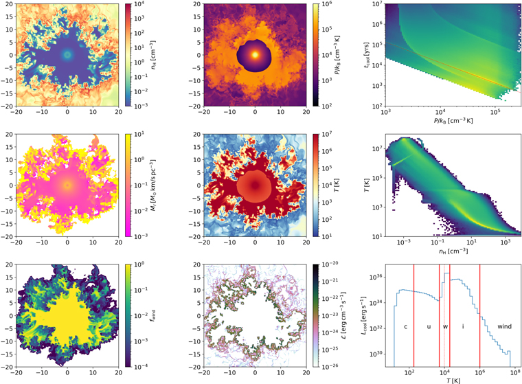
Figure 2. An example snapshot of the wind bubble structure and phase properties at time  after the initiation of the wind for the model with
  ,
,  ,
,  , and
, and  simulation. The left and center columns show slices through the z = 0 plane, while the right column displays distributions. From left to right and top to bottom, the panels show the gas number density, pressure, a cooling-weighted phase diagram of cooling time versus pressure, radial momentum density, temperature, a volume-weighted temperature-density phase diagram, the wind mass fraction (
 ), the cooling rate per unit volume, and a cooling-weighted histogram of the gas temperature distribution (which depicts the total cooling occurring in each temperature bin). In the top-right panel, the highest concentration of cooling is in gas that has
  this slope is indicated by a red dashed diagonal line for the coefficient in Equation (13) corresponding to
  . The last panel uses vertical lines to delineate the phases described in Table 2, where the subscripts from the table are indicated. The label “wind” includes both the free (f) and post-shock (ps) wind phases. In this panel,
  is marked as a vertical dashed line within the “w” phase.
Download figure:
Standard image High-resolution image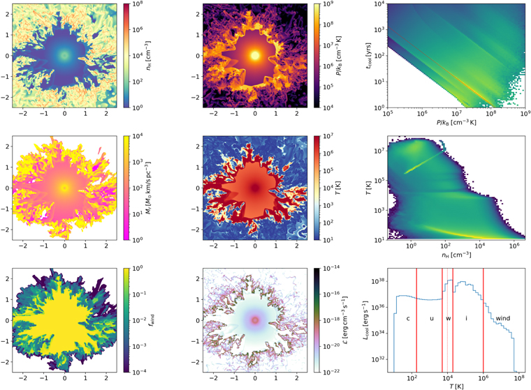
Figure 3. Same as Figure 2 but for the model with  ,
,  ,
,  , and
, and  simulation at
  . All quantities are as specified in Figure 2, though the range of many quantities are quite different.
Download figure:
Standard image High-resolution imageIn both figures, the wind-blown bubble is the low-density, high-temperature region filling the central region of the simulation domain, with fingers extending outward. Outside of the bubble, the inhomogeneous density structure generated by the background turbulence in the cold cloud is evident; higher density portions of the ambient gas are also left behind in the bubble interior, although they are ablated over time by KH instabilities as the high-velocity wind flows past them.
As expected, the cooling rate (bottom center panel) is greatest at the (fractal) interface between the hot bubble and cool shell, where mixing is driven by turbulence. The outward momentum originally carried by the wind is deposited at the bubble boundary by interface mixing, where it builds up in the expanding cool shell (middle left panel). The degree of mixing is also evident in the fraction of wind gas in each cell (bottom left panel).
Figures 2 and 3 also include (right column) information on the statistical distribution functions of gas in density, temperature, pressure, and cooling time. The top-right panel shows that the highest concentration of cooling is in gas with  , as predicted in Paper I (see definition in Equation (13)) . Quantitatively, we find that

follows well the prominent linear feature at short cooling time for both cases, as well as our other models. The corresponding  would be
  .
.
4.2. Gas Phase Definitions
We define several different gas phases as an aid in quantifying the structure and evolution of the wind-driven bubbles. These definitions can be thought of as an expansion on the phases laid out for the classical stellar wind bubble in Paper I, in order to better account for the cooling of the gas. These definitions (see Table 2) are based on the temperature T and radial velocity vr of the gas. The table also lists subscripts used to denote quantities associated with each phase (such as volume, momentum, energy, etc.). These subscripts label the thermal phases of the wind in the bottom-right panels of Figures 2 and 3.
Table 2. Definitions of Gas Phases
| Phase | Temperature Condition | Velocity Condition | Subscript | Schematic Region |
|---|---|---|---|---|
| Free Hypersonic Wind |

|

|

|

|
| Shocked Stellar Wind |

|

|

|

|
| Ionized Gas |

|

|

|

|
| Warm Neutral Gas |

|

|

| |
| Thermally Unstable Gas |

|

|

| |
| Cold Neutral Gas |

|

|

|
Note. Names assigned to gas phases based on temperature and velocity conditions, with (second-from-right column) the subscript used to denote each phase. The final column indicates the rough correspondence between gas phases and locations in the schematic in Figure 1(b) of Paper I.
Download table as: ASCIITypeset image
The first two phases listed in Table 2 are analogous to the two wind phases described in Weaver et al. (1977). The ionized gas is contained within the cooling layer, and cooling in this phase is dominated by collisional excitation of transitions of H, He, C, N, and O (primarily). This phase is produced via mixing and subsequent cooling of shocked wind and shell gas, and would not exist as part of the undisturbed/ambient ISM in either the uniform or turbulent cases.
The Warm Neutral Gas has cooling dominated by collisionally excited Lyα emission and recombination on dust grains. The Thermally Unstable Gas is in the range between the stable equilibrium warm and cold phases in the static case for our adopted cooling function. This phase is continually populated because of the turbulence in the system. Finally, at the lowest temperature there is the Cold Neutral Gas, which in reality would include both atomic and molecular phases, but here we do not follow the detailed chemistry.
The final three phases would all usually exist to varying degrees as part of the background in a turbulent, dense cloud. We wish to separate the portions that are ISM gas that has been shocked and then cooled after being swept into the expanding bubble shell from the portions that are undisturbed ambient gas. We do this using cuts based on the fraction of the mass in a given cell that originates in the wind,  . The wind mass is tracked using a scalar that is injected with the wind (see Section 3.1) and then passively advected.
For each of the Ionized, Warm, Thermally Unstable, and Cold phases of the gas we track all quantities of interest in gas with  and
and  (each subsequent selection being a superset of the previous selection). Unless otherwise stated, we use
  to separate the swept-up and ambient parts of these phases, as this gives the best agreement between different methods of measuring the total cooling, as described in Section 4.7. The tracking of gas properties at different
  values also allows us to quantify the mixing of the wind with the turbulent gas.
As is evident in the bottom-right panels of Figures 2 and 3, the majority of the cooling is occurring in the warm and ionized phases. These are the phases that primarily occupy the boundary region between the bubble and surrounding cloud, as is clear from the temperature and cooling slices in these figures.
4.3. Bubble Evolution Comparisons
Here, we present results from our simulations of the temporal evolution of the radial momentum of the gas ( ), the wind bubble’s effective radius (
 ), and the interior bubble energy (
 ). We compare these results with the theory developed in Paper I and reviewed in Section 2. When measuring quantities in the shell of the wind bubble, we include the measurement of this quantity in all gas with a wind mass fraction greater than 10−4. We found this was the best way of differentiating between the swept-up shell and the background gas.
In this section, we show results for the  cases, while results for other cloud masses are presented in Appendix C (Figures 24 and 25).
4.3.1. Shell Momentum
As is evident in Figures 2 and 3, most of the radial momentum is carried by the dense shell of swept-up gas, thus we define the momentum as

As mentioned above, only cells with a wind mass fraction greater than 10−4 are included in this definition. We found no significant changes in our measurement when considering  gas or even
  gas, which we took to indicate that there was no significant momentum carried in completely unpolluted gas. In Figure 4 (for the
  models), we compare this measurement of the momentum in the simulations with
  , as predicted by the EC theory with
  (Equation (3)).
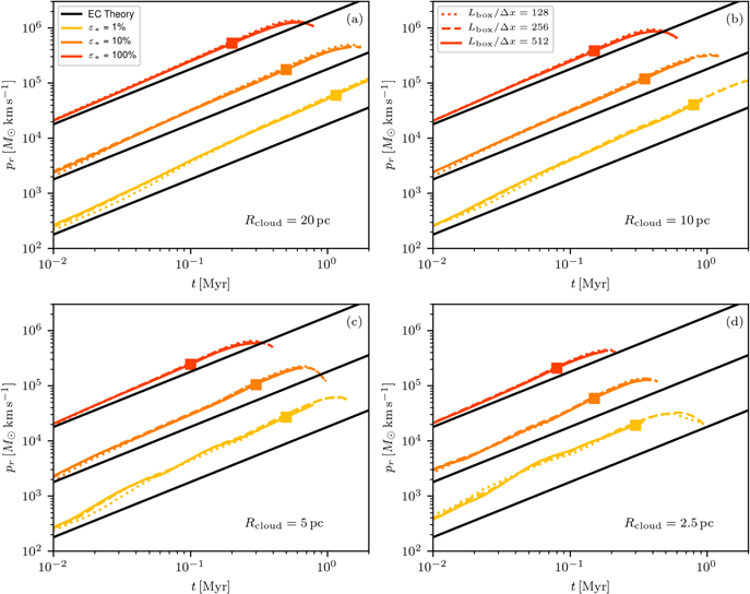
Figure 4. Evolution of the total radial momentum of the bubble (interior plus shell) in each of our simulations for cases with cloud mass  . Model cloud radii (from least dense,
  , to most dense,
  ) are given within the individual panels (a)–(d); see Table 1 for parameters. For each case, we show results for star cluster particles of mass M* = 103, 104, and
 (corresponding to star formation efficiencies of
  and 100%) in yellow, orange, and red respectively. At each value of
  and
and  we show three separate lines (solid, dashed, and dotted) corresponding to varying resolution, as shown in the key. For each simulation with 5123 cells, we mark the time at which the first wind-polluted gas exits the simulation domain
  with a square, and only show results from each simulation up until
  (though not all of the highest resolution simulations were run for this long). For each value of
  and
and  , we show
  (which should apply when cooling is maximally efficient, per Equation (3)) in black.
Download figure:
Standard image High-resolution imageThe results at different resolutions show that the radial momentum carried by the bubble is extremely well converged in our simulations. Overall, results are within a factor of 1.2−4 of the EC prediction. The results are quantitatively closest to  for more luminous winds (corresponding to higher star formation efficiency).
The momentum in excess of  can be attributed to nonzero buildup of thermal energy in the shocked wind that aids in driving expansion (see the Appendix of Paper I). This is parameterized in our theory by
  in Equation (3).
We note that once the bubble has reached the edge of the simulation domain (identified by nonzero outflow of wind-contaminated gas), we cannot expect the numerical solution to continue to follow the EC theoretical prediction. We mark this first blowout time in Figure 5 with large squares (for the highest resolution models). Some time after blowout, the rate of momentum increase falls below  because a fraction of the wind exits the domain without interacting with cloud gas.
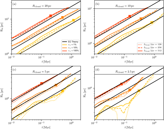
Figure 5. Evolution of the effective radius  in each of our simulations for cases with cloud mass
  . Line styles are as in Figure 4. For each value of
  and
and  , we show (in black) the evolution prediction from the EC theory (Equation (5), with
  ). The gray horizontal lines indicate
  , while squares indicate the time when wind-contaminated gas first leaves the domain (
 ). As in Figure 4, we only show simulation results up until
  .
.
Download figure:
Standard image High-resolution image4.3.2. Effective Radius
The effective bubble radius  is defined from Equation (4) based on the bubble volume,
  . For this volume, we include just the hot phases of the gas, the free wind (volume
  ), and the shocked wind (volume Vps):

Comparisons between our simulations with  and the prediction given by Equation (5) (with
  ) are given in Figure 5. It is clear that the EC theory very well explains the salient features of the radial expansion. The only exceptions are the smallest two clouds for
  , which is the least realistic parameter regime since high density regions are observed to have very high star formation efficiency (e.g., Leroy et al. 2018). These deviations are mainly caused by the Reynolds stress in the surrounding turbulent gas being non-negligible compared to the wind pressure, given the low
  .
.
We note in particular that the scaling  represents the numerical results better than the steeper scaling
  of Weaver et al. (1977) or El-Badry et al. (2019) for pressure-driven expansion. For the majority of cases that follow the
  scaling well, the numerical result is within 20% of Equation (5). Quantitatively, the EC theory works especially well at higher densities (where cooling is most efficient) and at higher
  (i.e., higher
  , where
  and
and  are larger, and therefore the constraint on Θ as given by Equation (14) is not as stringent).
At the time of first blowout, the mean bubble expansion rates range from  in the least dense cloud to
  in the most dense cloud, with larger velocities applying in the cases with higher wind power
  . Note that the first blowout (shown with colored squares) occurs much earlier than the time when
  (shown with a horizontal gray line) due to the fractal nature of the bubble interface, where parts of the bubble surface are at much larger radii than others.
4.3.3. Bubble Interior Energy
In keeping with the definition of the bubble interior given by Equation (26), we measure the bubble’s interior’s energy using

where the “ ” and “
 ” subscripts refer to kinetic and thermal energy, respectively. We note that the thermal energy within the free wind (
 ) is negligible compared to its kinetic energy, but we include it here for completeness.
Figure 6 compares the energy measurement from the simulations with the prediction given by Equation (6), employing Equation (5) and taking  . When comparing the theory and simulations, we see trends similar to those observed in the evolution of bubble radii and momenta: the EC theory is most accurate at higher
  and higher density
  .
.
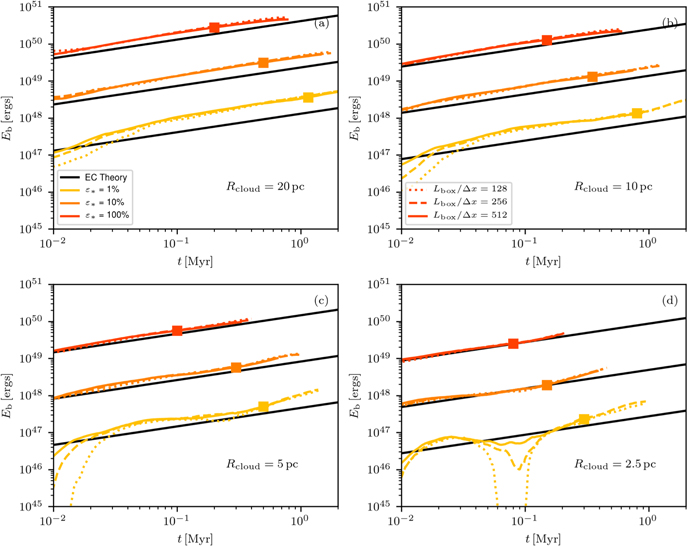
Figure 6. Evolution of the total energy in the interior of the bubble in each of our simulations for cases with cloud mass  . Line styles are as in Figure 4. For each value of
  and
and  , we show in black the energy given by Equation (6) (taking
  and using Equation (5)).
Download figure:
Standard image High-resolution imageWe also note that given the agreement with theoretical predictions for the shell momentum (as evidenced by Figure 4) and the bubble internal energy (as evidenced by Figure 6), we expect the shell’s radial kinetic energy to be half that of the bubble’s interior energy, as predicted in Paper I (see Equation (23) there). This is indeed the case.
4.3.4. Hot-gas Pressure
Finally, we compare the prediction for the pressure in the shocked wind gas given by Equation (7) and that measured in our simulations. We measure the pressure by selecting the shocked wind gas (conditions specified in Table 2) in simulation snapshots and calculating the volume-averaged mean thermal pressure. We use the  simulations for these comparisons as the pressure is computed directly from snapshots, which are taken at higher cadence in the lower resolution simulations. We also compute the
  ,
,  , and
, and  percentiles of the distribution of pressures in this gas.
In Figure 7, we compare the evolution of the pressure with the prediction of Equation (7). For this comparison, we use  , and we see that the theoretical prediction closely matches the evolution in the simulations. As we discuss below, the simulations actually have
  . From Equation (7) this would tend to increase the theoretical prediction (black curves in Figure 7), bringing the prediction closer to the observed simulation value for the low
  cases (which have the largest
  ), but further away from agreement for the high
  cases. The missing component here is the obliquity of the shock surface: the more oblique the shock, the less thermalized the shocked wind becomes, hence lowering the pressure (discussed at the end of Appendix A in Paper I). As is clear from Figures 2 and 3, the high
  winds have more oblique shocks, explaining this discrepancy.
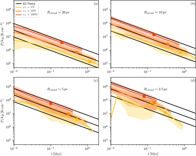
Figure 7. Evolution of the pressure in the shocked wind gas in cases with cloud mass  . All panels show the evolution of the volume-averaged mean pressure (solid colored lines) along with shading the 16th to 84th percentiles of the distribution of pressures in post-shock gas (colored shaded regions). We show the theoretical prediction (Equation (7), with
  ) in black. The time at which wind first escapes the domain is indicated by a colored square.
Download figure:
Standard image High-resolution image4.4. Dimensionless Parameters
In the above comparisons we explicitly set the dimensionless, order-unity parameters of our theory equal to unity. However, the values and time evolution of these parameters provides interesting insight into the validity of the assumptions in the EC theory for different regimes (see Section 4.3). As is explained in Appendix A of Paper I and summarized in Section 2, some of these parameters are interdependent.
The first dimensionless parameter is  , which is defined as the rate of momentum input to the surrounding medium divided by the rate of momentum injection by the wind. Specifically, we measure

where  is as measured in Equation (25). This measurement of
  is shown as solid lines in Figure 8.
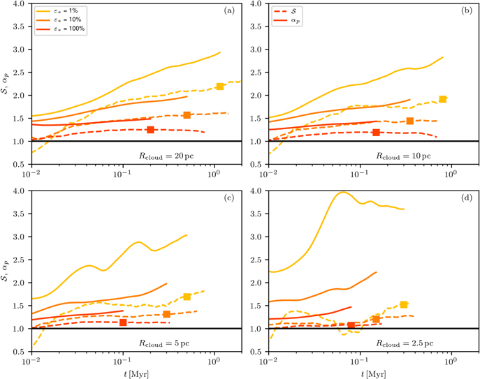
Figure 8. Evolution of the momentum ( ) and energy (
 ) enhancement factors shown as solid and dashed lines, respectively. The evolution of
  is only shown up to the point of breakout, which is indicated with colored squares on the curves for
  . We indicate the no enhancement case with the horizontal black line. We show the highest resolution version of all simulations with
  .
.
Download figure:
Standard image High-resolution imageAnother quantity in the EC theory is the energy enhancement factor  , defined in Equation (6). As explored in-depth in Appendix A of Paper I,
  and
and  are expected to track each other (with
  ) because both are associated with buildup of energy in the bubble interior. For the same reason, we expect
  to be higher when the shocked wind makes up a larger portion of the bubble volume, i.e., larger
  . We also expect larger
  when shock surfaces are less oblique. In order to directly compare
  with
with  , we show in Figure 8 a measured value of
  as dashed lines.
The measured value of  is taken as the ratio of the bubble energy in the simulations, measured according to Equation (27), to
  , where
  is taken as the fixed wind momentum input rate and
  is computed from the simulations as detailed in Section 4.3.2.
The next dimensionless parameter we introduce is  , which encodes geometric factors. Using Equation (5),

We evaluate this using the measured  (see Section 4.3.2) and
  (Equation (28)). We note that we have no explicit theoretical prediction for
  other than expecting it to be near unity. Figure 9 shows the measured values of
  over time. We see that
  remains quite close to unity, remaining in the range 0.5–1.5 for the majority of the evolution. There is also some indication that
  takes on lower values in the higher density clouds.
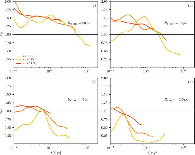
Figure 9. Evolution of the dimensionless parameter  . Line colors are associated with simulations of different
  . We use the highest resolution version of all simulations with
  and only show the evolution up to the point of breakout (square markers in Figure 4 and others).
Download figure:
Standard image High-resolution imageThe radial kinetic energy of the shell in the EC theory is determined by momentum input from the wind, but there is no prediction for the kinetic energy in non-radial, turbulent motion. Given that the theory relies on efficient cooling facilitated through a turbulent interface, we expect a significant fraction of the kinetic energy in the shell (and around the bubble/shell interface) to be in turbulent motion. The simplest way to quantify this is in terms of the  parameter defined in Equation (9).
To measure this parameter we write the total radial kinetic energy in the shell as

where the sum is performed over the indicated phases, and as in Equation (25), we sum over zones where  . The total kinetic energy is measured in an analogous way.
The ratio  is displayed in Figure 10. Surprisingly, for much of the bubble evolution and most of the parameter space, the energy in turbulent motion is at least as large as the energy in radial motion, with
  (equipartition between radial and turbulent motion) over much of the parameter space. This fact emphasizes how important the turbulence is for the evolution of the bubble, especially the turbulence driven by the wind. We observe that the more powerful winds instill a larger fraction of their kinetic energy in radial motion.
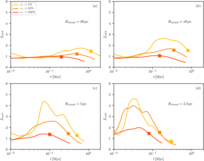
Figure 10. Evolution of the ratio of turbulent kinetic energy to kinetic energy in radial motion, for shell gas. We show the highest resolution version of all simulations with  . The square symbols mark the point at which wind-polluted mass begins to leave the domain.
Download figure:
Standard image High-resolution imageIn all simulations the fraction of turbulent kinetic energy in the shell increases in time until seemingly reaching a set value before decreasing again. As we will see upon further inspection of the turbulent motion below, this reflects a saturation of turbulence as more and more radial energy is provided to the wind.
4.5. Turbulent Structure Function
Both the amplitude and spectral shape of turbulence are important to the mixing and cooling that dictate the bubble evolution. These are quantified via the turbulent structure function.
Following the theory outlined in Paper I, we particularly wish to measure the turbulence in the hot gas near the interface. To this end, we select gas with  and
and  (the Ionized Gas and the Shocked Stellar Wind). In order to isolate the turbulent motion from the bulk radial outflow in this gas, we apply our structure function analysis only to the non-radial components of the velocity field. We will refer to this proxy for the turbulent velocity field (which is really the tangential velocity field) as
  defined as

where  is the full velocity field. Of course, there are also turbulent contributions to the radial motion, but directly quantifying this is problematic due to contamination by the strong background radial flow. Figure 11 shows example snapshots of the magnitude of
  from the
  model (in the purple-to-yellow color scheme).
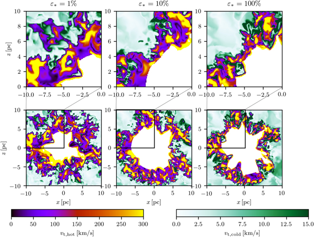
Figure 11. Magnitude of the tangential velocity in snapshots of the  models at the time in each simulation when
  . The separate columns (left to right) are the
  and 100% cases. The hot gas (Shocked Stellar Wind and Ionized Gas) is shown with the purple-to-yellow color scale, while the cool gas (warm, thermally unstable, and cold gas) is shown with the green color scale. The top row of panels is a zoom-in of the bottom row, which itself zooms in on just the bubble region, to highlight the structure of turbulence in the bubble/shell interface.
Download figure:
Standard image High-resolution imageTo measure the turbulent structure function, we randomly select a cell i from the region under consideration. We then compute two histograms. The first histogram is the number of cells at position j with a spatial separation  from cell i, binned by width
  . The second histogram is as above, except now the histogram is weighted by the square of the difference in the tangential velocity field between positions i and j:

Dividing the second histogram by the first and taking a square root gives us a single sampling of the root-mean-square velocity offset as a function of separation scale ℓ. In order to account for the (unmeasured) radial component of the true turbulent velocity field, we additionally multiply by  (assuming that the turbulence is isotropic). We repeat the above process for 200 cells randomly selected from the Ionized Gas and Shocked Stellar Wind .
With this factor of  we refer to the measured structure function as
  . With these 200 samples of
  we take the median value in each radial bin (over the ensemble of samples) to represent the structure function. We also calculate the 25th to 75th percentiles over these 200 samples to quantify the width of the distribution of velocity deviations at each scale.
As the calculation described above is quite computationally expensive, we only calculate the full time evolution of the structure function for a subset of our simulations ( ,
,  , and
, and  ). The results of these calculations are illustrated in Figure 12, where the turbulent structure function is shown in time increments of 104 yr varying from early times (shown in dark blue) to late times (shown in bright green). The beginning time is
  and the ending times are 2.23, 1.21, and
  for the
  10%, and 100% cases, respectively. At all star formation efficiencies the characteristic velocity scale of the turbulence decreases in time but only by at most a factor of 2. In comparison, the shell velocity decreases by a factor of 10 over the same time interval.
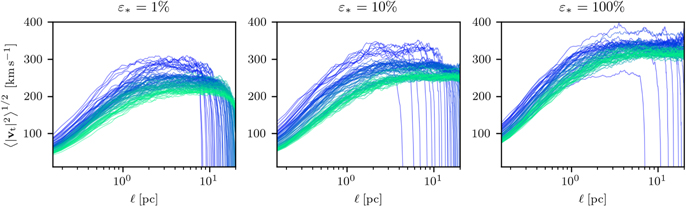
Figure 12. Temporal evolution of the structure function of turbulent velocities in the hot gas (Shocked Stellar Wind and Ionized Gas ) in the first  of the simulation for the
  and
and  simulations. The separate panels (left to right) are the
  and 100% cases. Temporal evolution is indicated by the color of the lines in each panel, moving from early times (dark blue) to the late times (bright green) in increments of
  . The characteristic velocity scale of the turbulence decreases in time and varies by at most a factor of 2 over the course of the simulation. The characteristic spatial scale of the structure function increases over time. Turbulent velocities are overall higher for the higher wind power (
 ) models.
Download figure:
Standard image High-resolution imageFor the rest of our simulations with  and
and  , we measure the structure function of the turbulence at the individual time when
  . We show these structure functions, along with the 25th to 75th percentiles of velocity deviations, in Figure 13. To provide a reference for the background turbulence, we calculate in the same way the structure function of the turbulent background in the full simulation volume just before the initiating of the wind. This background turbulence has a much lower velocity than the turbulence in the hot gas, so we scale the background measurements by a factor
  this scale choice is purely for plotting purposes. This scaling also adjusts for the differences in initial turbulent velocity scales
  among the different size clouds (as laid out in Table 1) so that all background structure functions appear essentially identical.
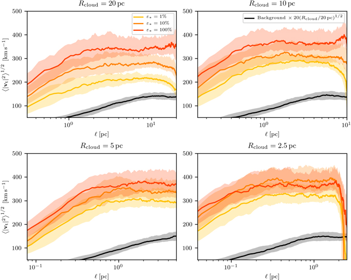
Figure 13. The structure function of turbulent velocities in the hot gas (Shocked Stellar Wind and Ionized Gas ) when  . These are measured in the highest resolution versions of all simulations with
  and we show the simulations with ε* = 1%, 10%, and 100% in yellow, orange, and red, respectively. For each panel we show scales from
  to
to  (solid lines) as well as the 25th to 75th percentiles of structure function measurements over the ensembles of 200 samples from the hot gas. In each panel we show in black the structure function of the background turbulent gas scaled up by a factor
  . The velocity scale of the turbulence is set by the strength of the wind (represented here by
  ) while the characteristic length scale of the turbulence is likely set by the bubble size and turbulent density structure of the background.
Download figure:
Standard image High-resolution imageIt is clear from Figure 13 that the velocity scale of the turbulence is determined primarily by the strength of the wind, which is represented here by  . However, the characteristic spatial scale of the turbulence, which is where the structure function flattens out, is consistently
  , suggesting that this scale may be set by the size of the bubble and/or the spatial scale of the background turbulence. This variation in turbulent velocity magnitude with
  could be explained by the more oblique shocks in the higher
  cases: when a shock is more oblique, the post-shock flow will have a larger speed.
Along those lines, we note that for the  case in the
  cloud, the amplitude of the turbulent velocity is lower than expected. This is because the
  restriction cuts out much of the shocked wind due to the strongly oblique shocks in this case (see Figure 3).
4.6. Fractal Structure of Interface
In this section we explore the fractal nature of the bubble/shell interface. These results also inform the discussion of turbulence-induced mixing and cooling in Paper I.
4.6.1. Fractal Dimension from Cooling
We measure the fractal dimension of the bubble surface in two different ways. Since the details of the fractal structure of the bubble/shell interface affect the cooling, it makes sense to measure the fractal dimension using the cooling itself. To that end, we determine the fractal dimension using a box-counting or Minkowski–Bouligand algorithm (Schroeder 1991) where membership in or out of the fractal is determined based on cooling.
2
To maximize the dynamic range we use simulations with  . To be consistent with the turbulent structure function measurements of Section 4.5, we analyze the fractal structure at the time when
  .
.
We first choose a fraction  . For a given time snapshot we measure the total amount of cooling,
  . We denote
  as the cooling rate in the
  hydrodynamical cell, for a sorted list starting with the maximal cooling rate. We then compute the cumulative sum up to I such that
  . The count I of cells contributing to the specified cooling fraction at the minimum scale
  (the resolution of the simulation) is hereafter denoted by
  .
.
We next reduce the size of the simulation grid by a factor of 2 in each direction, so that merged cells have length  , and the cooling of adjacent cells is combined. We repeat the above sort-and-accumulate process to measure the number of cells
  needed for
  . We iteratively repeat this process for
  and 32 and use these measurements to calculate the fractal dimension as

This quantity will vary with scale, ℓ. However, we expect d to take on a roughly constant value on large scales, dropping below this at sufficiently small scale due either to limited numerical resolution or to some physical dissipation scale such as the cooling length,  . In practice the former is more relevant as the cooling length is usually below our resolution limit.
At sufficiently large  , d is close to zero on large scales and becomes very large (based on our fitting method) on small scales. This is because
  becomes a very steep function of
  when transitioning beyond the concentrated cooling in the interface boundary layer. Above a certain
  , essentially the whole domain is included, implying that the true
  at small ℓ.
We believe that the most physical d to associate with the fractal structure of the cooling interface is the value at large scales for the largest value of  that does not exhibit the discontinuous behavior explained above. On the left-hand side of Figure 14, we therefore show the dependence of d on scale for the largest choice of
  that does not result in this discontinuous behavior. This choice of
  varies between simulations.
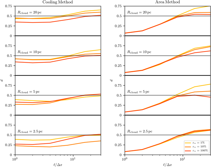
Figure 14. The excess fractal dimension of the bubble surface as a function of scale using the two measurement techniques described in the text (see Sections 4.6.1 and 4.6.2). Left panel: the excess fractal dimension of the bubble surface measured using a box-counting technique; boxes at different scales mark where cooling is taking place. Right panel: the excess fractal dimension measured based on the logarithmic scaling of the area of an isotemperature surface ( for all curves shown here) when measured on different scales.
Download figure:
Standard image High-resolution imageThe scale-dependent nature of the excess fractal dimension d is evident in Figure 14, where d decreases at small scales. We see that d tends to be larger at smaller values of  (this is clearest in the larger/lower density clouds). In part, this may be because turbulence at the bubble/shell interface, which is responsible for creating the fractal structure, makes up a much larger fraction of the kinetic energy at low
  , as was shown in Figure 10.
Overall, this measurement method suggests a fractal dimension  in most simulations, with larger values (up to ∼0.6–0.7) in models with very low
  and large
  .
.
4.6.2. Fractal Dimension from Isotemperature Surfaces
Our second method of measuring the fractal dimension, paralleling Fielding et al. (2020), uses the area of isotemperature surfaces for temperatures that should be characteristic of the interface between the wind bubble and the shell. Specifically, we measure the area of isotemperature surfaces for  ,
,  , 105,
  and
and  . We use the marching_cubes algorithm from the scikit-image package to measure these surface areas, using step sizes
  and 32.
The excess dimension d is then given by the logarithmic derivative of the area with respect to the scale on which the area is measured

As with the previous method, this value should be a constant over a large range of scales, decreasing at some small scale due to numerical or physical dissipation (usually the former). Our measurements are made at the time when  . The scale-dependent results are shown on the right side of Figure 14. For the sake of brevity, we only show the results for the isotemperature surfaces measured at
  for each simulation.
Figure 14 clearly shows that this measurement technique consistently finds  at small scale, as expected. We also found (not shown) that the value of d on large scales depends on temperature: the higher temperature surfaces have more fractal (higher d) structures than the lower temperature surfaces, with the effect most extreme in the smallest-
 , largest-
 models. On large scales, the range of d from this technique falls roughly within
  .
.
It is also interesting to note that at all cloud sizes, the bubble surface tends to become less fractal at higher wind luminosity (or  ), as seen in the previous measurement technique, but now to a higher degree. Physically, the more-fractal structure in the lower-
 models at large scales may potentially be explained by their greater buildup of hot gas (higher
  ), which can more effectively create fingers of high-temperature gas within the lower density parts of the turbulent cloud at large scales.
4.6.3. Area Measurements
Using the results of Section 4.6.2, we can now assess the relationship between the bubble’s surface area and its effective radius,  , as defined by Equation (11). In particular, this allows us to test whether a single fractal dimension can describe the surface and to evaluate the free parameter
  in that equation. For this analysis we consider the models with
  and
and  at all values of
  .
.
We set

where  denotes the scale-dependent area measurement of the isotemperature surface (at a range of T), and ℓ is the measurement scale. We shall use
  , the scale on which the fractal structure begins to saturate (as is evident in Figure 14). Equation (35) compares the actual area with the prediction for a fractal with excess dimension
  as this value is broadly consistent across the range of parameters investigated and measurement techniques used.
We present the time evolution of Equation (35) in Figure 15. Especially for the larger  cases, we conclude that the simple
  fractal agrees extremely well with bubble’s true surface area.
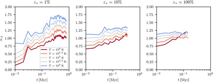
Figure 15. The ratio of bubble surface area  to fractal area
  as
as  evolves in time. We only show the evolution up to the point of wind breakout. We set
  and measure the area for several isotemperature surfaces as marked in the key. Results for
  from taking the area ratio (see Equation (35)) are shown for
  ,
,  , and
, and  and
and  . The near constancy of
  in time, especially at
  and 100%, is an excellent indication that a fractal with
  describes the geometry of the bubble well.
Download figure:
Standard image High-resolution image4.6.4. Bubble Geometry
Finally, we consider an additional characteristic of the bubble geometry, which we term its foldedness. We define this as the value of the dot product of the unit normal to the bubble surface ( ) and the unit radial vector (
 ). There are physical reasons that this quantity matters. In the spherically symmetric, pressure-driven bubble of Weaver et al. (1977), El-Badry et al. (2019), and others, the bubble expands due to a pressure gradient force normal to the bubble surface. Since the bubble is spherical, the normal vector to the surface is always directed exactly radially outwards, so that the pressure force and expansion velocity are exactly aligned. In the case of a bubble in a turbulent medium, the surface will have a complicated geometry, as Figures 2 and 3 illustrate. For any pressure force acting normal to the bubble surface, only a fraction of the force will act radially outward. The radial contribution from a normal force can be then be quantified by this foldedness quantity
  .
.
The quantity  is our measure of the foldedness of the surface in the case of our wind-driven bubbles, and this is important in setting the radial force that drives the overall expansion. Specifically, if there is a uniform internal pressure P, the effective outward radial force on the bubble surface can be written as

for an appropriate effective area,  . We define
  using the area of isotemperature surfaces
  from Section 4.6.2 and the foldedness
  as
as

Again, using the marching-cubes algorithm, we evaluate  by taking the dot product of the unit normal to each triangular face output by the algorithm with the unit radial vector pointing to the center of that triangular face. We then average these values over the set of faces. The results are displayed in Figure 16 for the
  ,
,  model at all values of
  . In Figure 16, we also show that the scaling of
  in time is very similar to the temporal behavior of
  . Both of these quantities decrease in time
  . But more important than the specific time dependence is the fact that the scaling of the excess fractal dimension is compensated by the foldedness of the surface, such that
  .
.
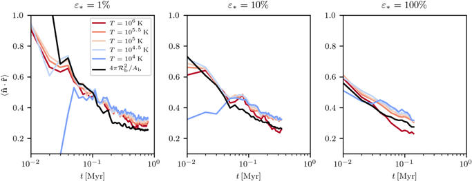
Figure 16. The average value of the dot product of the outward normal vector to the bubble surface with the radial vector, which we term the foldedness of the bubble surface. The degree to which this is less than one quantifies the amount that the surface is inward facing or crumpled. The same models are used as for Figure 15, along with the same calculations of the bubble isotemperature surfaces. We also show  in black. The degree to which the black curve matches the other curves reflects how close the effective area,
  is to the equivalent spherical surface
  .
.
Download figure:
Standard image High-resolution imageOur findings on scalings imply that the effective area for radial pressure forces is the same as for a spherical surface. We posit that this property is generally true. That is, for any bubble, the quantity  defined in Equation (37) scales as the square of its associated linear scale defined through the cube root of volume. Though the divergence theorem can be used to show that
  for
for  the bubble radius at a given spherical polar angle, we have not found proof to connect this to Equation (4); nevertheless, it seems intuitively reasonable.
The above proposition that  points to the self-consistency of the assumption in the EC solution that the angle-averaged radial force in the momentum equation does not explicitly depend on detailed geometry, even for a fractal bubble. It is the combination
  that drives outward expansion of the bubble. The Reynolds stress term is radially directed and therefore always contributes to the shell momentum in the
  direction, but the pressure term would produce a normal force where it acts on the shell, and therefore would contribute to the radial momentum as in Equation (36). Our conclusion that
  is then what allows us to treat the total momentum input rate via an equivalent spherical calculation, with the breakdown of the two contributing terms provided in the Appendix of Paper I (see Equation (A11) there).
4.7. Cooling and Energetics
4.7.1. Measured Cooling and Retained Energy
Energy inputs from the wind are split between the (thermal and kinetic) energy in the interior of the bubble,  , the radial kinetic energy of the shell,
  , the turbulent kinetic energy in the shell,
  , and energy that is lost to cooling,
  . The EC theory presented in Paper I and reviewed in Section 2 provides predictions for
  and
and  and thus (through the total input energy
  ) for the sum of the energy lost to cooling and the energy in turbulent motion. The exact split between turbulent energy dissipation and cooling is not predicted by our theory, but we can account for it in simulations using the quantity
  , introduced in Section 2 and shown in Figure 10. In this section we will endeavor to measure the cooling that is occurring in our simulations directly and check that this is consistent with the prediction given by Equation (10).
First, we must measure the cooling directly from the simulations. Since, however, there is cooling present in the background gas, mixing between the background gas and the wind, and cooling occurring in the background gas that is shock accelerated by the wind, this is not a trivial task. The measurement is further complicated by the fact that the cooling will be a large fraction of  , so that an inclusion of only a small amount of background cooling in our measurement can make our inference of
  greater than 1. To address these issues we proceed by measuring the cooling in two separate ways so that we may check for consistency between our methods.
The first way follows our method for measuring momentum, as laid out in Section 4.3.1. Specifically, we sum the cooling in all gas with  in our simulations. The justification of this otherwise arbitrary cut in
  is based on the excellent agreement among measurements of the radial momentum at different resolutions when using this criterion, as evidenced in Figure 4 and also its agreement with our second measurement method, detailed below.
We measure the cooling in another way by using conservation of energy. The time derivative of the total energy in the simulation domain can be written as

where  is the sum of cooling that occurs in the swept-up ambient gas and the bubble/shell interface,
  is the rate at which energy moves out of the simulation domain through the boundaries, and
  is the net cooling (=cooling—heating) in the ambient gas that is not due to the wind. While it is straightforward to measure the total energy in the simulation domain, and hence its time derivative
  , as well as the rate at which energy leaves the box, it is not so easy to define what the cooling due to the background ambient gas is.
We address this by running the simulations that we initialized before turning on a wind (as described in Section 3.2) forward in time without a wind and measuring the net cooling that occurs throughout the volume. We will denote the cooling that occurs in these simple turbulent evolution simulations as  . To account for the fact that part of the simulation volume that would normally be cooling as background gas will have been displaced by the wind bubble in our simulations, we measure
  as
as

With this measurement of the background cooling we can use Equation (38) to determine  .
.
The results of the two methods for calculating  are displayed in Figure 17 as solid and dotted lines for the
  ,
,  and
and  cases, for all
  values. We only show these lower density cases as, in the higher density simulations, the background cooling becomes too strong and difficult to separate from the cooling associated with the wind, especially at low values of
  . In fact, this effect is already evident in the
  and
and  case shown in the bottom left panel of Figure 17.
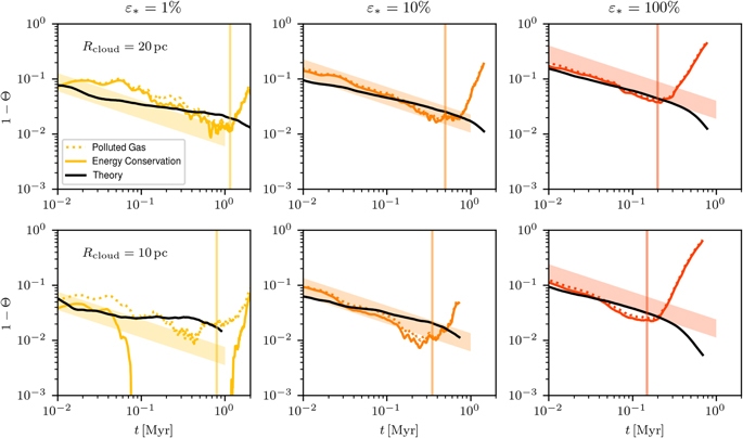
Figure 17. The fraction  of the input wind energy that is retained in the bubble and shell, including both kinetic and thermal terms, as a function of time. We show results for the
  in the top row and
  in the bottom row (both with
  ), for
  and
and  . The time when the wind breaks out of the simulation box is denoted in each panel by a colored vertical line. The colored solid lines in each panel denote
  measured via the energy conservation method, while the dotted lines denote the same quantity measured using cooling in wind-polluted (
 ) gas. The shaded areas in each panel delimit the range expected from EC wind theory (see text). The black line in each panel shows the theoretical prediction from Equation (10) with values of
  ,
,  ,
,  , and
, and  determined as described in Section 4.4.
Download figure:
Standard image High-resolution imageThere is excellent agreement between our two measurement methods, with only moderate deviations at low  values. The dramatic increase in
  (decrease in cooling) toward the end of each simulation can be attributed to breakout and venting of the wind outside of the simulation domain, the onset of which is indicated by the colored vertical line.
In Figure 17 we also show, as indicated by the shaded region in each panel, where we expect the solutions for  to lie. This is bounded above by the locus at which the EC condition applies as given by Equation (14), and bounded below the locus of maximum cooling as given by Equation (10) with
  and
and  , so that the right-hand side becomes
  . Both of these limits have retained energy fraction
  with different coefficients (3.8 and 1.5, respectively), decreasing in time as
  . Finally, as black lines, we show the prediction of Equation (10) in its entirety, with time-varying values for
  ,
,  ,
,  , and
, and  measured as described in Section 4.4.
Overall, Figure 17 shows that the different numerical measurements of  are in good agreement with each other and with theoretical estimates. At early times (
 ), the energy retained in the bubble amounts to
  of the input, slightly increasing for lower density clouds and for more powerful winds (larger
  ). This decreases
  until the time breakout occurs,
  (decreasing at higher wind power and for denser clouds).
4.7.2. Total Possible Cooling
Finally, we connect our results to the expected requirements for the EC solution based on the theory of cooling and mixing at turbulent, fractal interfaces, as discussed in Paper I. To this end, we measure two quantities. The first is the expected radial velocity of shocked wind gas being advected to the boundary mixing layer ( , given by Equation (15)). The second is the equivalent velocity of gas flowing through the mixing/cooling layer, as given by Equation (12); this takes into account the fractal structure of the bubble surface, but is only really defined up to a multiplicative factor from our theoretical analysis.
For this exercise, we use the time dependent measurements for the evolution of the bubble’s effective radius (Figure 5), the shock radius ( ), and the turbulent structure function (Figure 12) in models with
  ,
,  , and all
  . We choose
  and calculate
  . Note that we have implicitly adopted a fractal dimension of
  , which is broadly consistent with our results in Sections 4.6.1 and 4.6.2. As noted above, the equivalent velocity in Equation (12) is only predicted up to an order-unity coefficient. We therefore multiply
  by a factor 0.25 and show the results of this calculation in Figure 18.
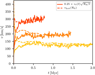
Figure 18. Evolution of quantities related to the flow into and through the turbulent mixing/cooling boundary layer between the bubble and the background. The expected radial velocity (Equation (15)) of shocked wind gas advected into the fractal interface is shown as dashed lines. The equivalent velocity of gas transiting the mixing/cooling layer (Equation (12) with  ) is shown as solid lines, including a factor of 0.25 chosen to match the dashed lines. These curves are shown for the model with
  ,
,  , and all
  . We use
  for the measurement scale of the turbulent structure function.
Download figure:
Standard image High-resolution imageFigure 18 shows that there is excellent agreement between the expected velocity at which energy and mass arrives at the surface of the bubble (an advection speed), and the effective flow velocity through the mixing/cooling boundary layer (a diffusion speed). This directly demonstrates a key feature of our model: all thermal energy that is delivered to the turbulent interface is efficiently mixed in and radiated away as rapidly as it arrives.
5. Summary and Conclusion
In Paper I, we described a theory for the expansion of a stellar wind-driven bubble into the dense, turbulent ISM, characterized by strong cooling losses due to turbulent mixing of the hot gas with denser gas at the bubble surface. We posited that this cooling was large enough to cause the dominant phase of the bubble’s evolution to be momentum driven.
A solution in which momentum input (rather than energy input) controls bubble evolution has been discussed in the past by several authors in various contexts (Steigman et al. 1975; Ostriker & McKee 1988; Koo & McKee 1992a, 1992b; Silich & Tenorio-Tagle 2013; Kim et al. 2017), and others have suggested that such solutions could be associated with efficient mixing and cooling at boundary layers (Garcia-Segura et al. 1996a; Dale & Bonnell 2008; Mackey et al. 2015; Fierlinger et al. 2016), but none have previously demonstrated that this regime generally applies within star-forming molecular clouds. We do this by conducting a large suite of 3D hydrodynamic simulations with winds injected into dense, turbulent ISM material. Analysis of our simulations shows that the predictions of our theory very accurately describe the evolution of the wind bubble’s volume, the momentum that it carries, and its energetics. Our simulations demonstrate that the limit of maximally efficient cooling in our theory is most appropriate for the strongest stellar winds (parameterized in our model by high values of the star formation efficiency  ).
).
Our theory and simulations explore in detail where energy is stored and explain physically how most of it is radiated away, via processes analogous to those that have been investigated in recent simulations of KH unstable mixing layers with fractal geometries (e.g., Fielding et al. 2020; Tan et al. 2021). The fractal theory of the bubble interface also accurately predicts essential quantities of the bubble such as the area of its interface with the ambient ISM and properties of the geometry of this interface. We additionally demonstrate that it is the fractal nature of the bubble that allows for such efficient cooling by showing that the cooling capacity under our fractal theory is consistent with the energy being provided by the stellar wind.
The main conclusions from our simulations can be summarized as follows:
- 1.
- 2.The total momentum carried by the bubble increases approximately linearly in time (Equation (3)) and is typically only slightly larger (at most a factor 4) than the total momentum injected by the wind, with the smallest enhancement for the most luminous winds (largest
 ), as shown in Figure 4. The momentum enhancement factor reflects buildup of hot shocked gas within the bubble; higher turbulence levels in models with more powerful winds drive stronger interface mixing and limit this buildup, keeping very close to unity.
 - 3.From analysis of the shells in our simulations, we find (see Figure 10) that the energy carried in tangential motion is typically greater than that carried in radial motion (turbulence dominated). These results show that shells typically become more turbulence dominated in time up to the point of bubble breakout from the simulation domain. We also find that cases with less luminous winds and denser environments are more turbulence dominated.
- 4.We measure the turbulence in the hot gas directly, and find typical velocities of 150–350 km s−1 (amplitude increasing with input momentum rate; see Figure 13), which are about 10%–15% of the wind velocity. This turbulence has characteristic energy-containing or outer scale that is larger in larger clouds (Figure 13), suggesting that the background inhomogeneity induced by turbulence helps to define it. The outer scale is typically ∼10% of the bubble size, growing with the bubble (Figure 12).
- 5.We quantify the excess fractal dimension d of the bubble/shell interface in two different ways (see Figure 14), and find that this generally falls in the range of. Lower luminosity winds generally have higher fractal dimensions, which is consistent with the shells driven by these winds being more turbulence dominated, as it is the turbulence that induces the fractal structure. We also find that the fractal characterization of the shell interface is in excellent agreement with the measured area (Figure 15) and geometry (Figure 16).
- 6.We use to denote the fraction of the energy input rate from the wind that remains in the bubble as either thermal or kinetic energy at any given time. We find that , decreasing in time (Equation (10)) for all models (Figure 17). The very small value of is consistent with observational constraints (see Paper I discussion).





We have demonstrated that our simulations are well converged in all of the quantities that we investigate here. Higher resolution should only increase cooling, so we believe our results for the efficient-cooling bubble evolution solution are robust. However, our present simulations do not resolve the scale  at the wind bubble interface where mixing and cooling timescales would be comparable in the real ISM. Full validation of the small-scale processes discussed here will therefore require higher resolution simulations, an important direction for future work.
Finally, we reiterate that the simulations presented here include only a limited set of the relevant physical processes. In particular, we have not included radiation or magnetic fields. EUV radiation would photoevaporate gas from the shell surfaces that face the cluster, while FUV radiation absorbed by dust (where it is not destroyed) directly deposits photon momentum; both effects drive expansion of the bubble surrounding the cluster. The free wind and shocked wind regions would then in general interact with photoionized gas that has been evaporated from the shell, rather than directly with the denser shell gas (e.g., Dwarkadas & Rosenberg 2013; Geen et al. 2021). With a lower density contrast, KH instabilities at hot/warm interfaces would have higher growth rates than for hot/cold interfaces at the same pressure. The turbulent mixing process would likely occupy a larger volume of photoionized gas compared to the situation here, since the turbulence levels in the interaction region depend on the density contrast (Fielding et al. 2020). Magnetic fields presumably also affect the mixing/cooling process. Given the extremely high velocities of the shocked wind, field strengths in the cloud would have to be very (unrealistically) high to prevent primary instabilities at the interface, but magnetic tension could still limit the turbulent cascade at small scales (and render it anisotropic). Numerical magnetohydrodynamic studies including both winds and radiation will be needed to assess how the turbulent mixing/cooling process and overall dynamical evolution are quantitatively affected.
We thank Drummond Fielding and Erin Kado-Fong for useful discussions. We thank the referee for many insightful comments that improved the quality of the manuscript. This work was partly supported by the National Science Foundation (AARG award AST-1713949) and NASA (ATP grant No. NNX17AG26G). J.-G.K. acknowledges support from the Lyman Spitzer, Jr. Postdoctoral Fellowship at Princeton University. Computational resources were provided by the Princeton Institute for Computational Science and Engineering (PICSciE) and the Office of Information Technology’s High Performance Computing Center at Princeton University.
Software: Athena (Stone et al. 2008; Stone & Gardiner 2009), Astropy (Astropy Collaboration et al. 2013, 2018), SciPY (Virtanen et al. 2020), NumPY (Harris et al. 2020), IPython (Perez & Granger 2007), Matplotlib (Hunter 2007), xarray (Hoyer et al. 2017), pandas (Reback et al. 2020), adstex (https://github.com/yymao/adstex).
Appendix A: Validation of Wind Implementation
We test our implementation of stellar winds by comparing to analytic solutions given by Weaver et al. (1977) for a spherical wind expanding into a uniform, static background medium. In our test the background medium has a number density of  . The wind has a mechanical luminosity of
  and a mass-loss rate of
  . This corresponds to a wind velocity of
  . The simulation was run in an
  box with 1283 cells. The feedback radius was set as
  (
( ), and we used
  subcells. We run simulations both with and without cooling (the latter is fully adiabatic). The results of these tests are displayed in Figure 19.
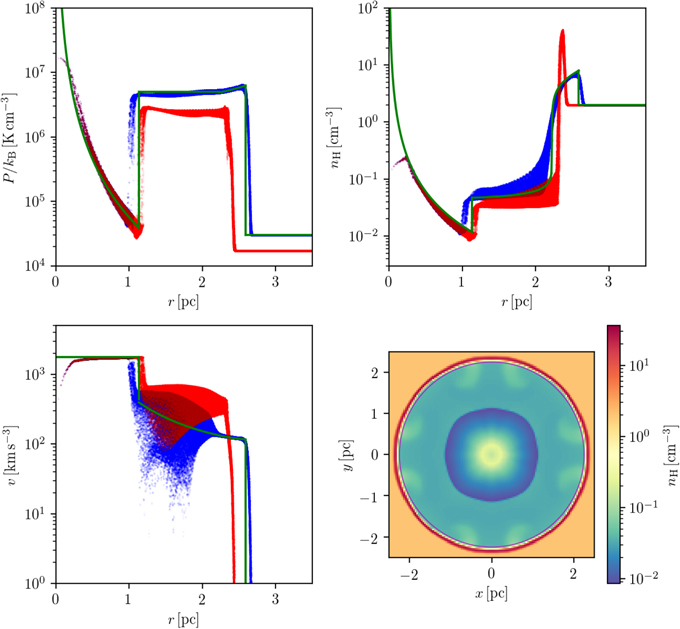
Figure 19. Wind implementation tests for a uniform background, shown for a snapshot 104 yr after the start of wind feedback. We show profiles (every cell is plotted) of pressure (top left), number density (top right), and velocity magnitude (bottom left) in radius for both the adiabatic run (in blue) and the run with cooling (red). The Weaver et al. (1977) solution for fully adiabatic evolution is shown in green for these same panels. In the bottom-right panel, we show a slice of number density through the z = 0 plane of the simulation for the run with cooling. One can clearly see the cooled, dense shell that has formed at the outer edge of the wind bubble. The Weaver et al. (1977) solution for the radius of the shell in the case that gas in the leading shock cools is indicated as a magenta circle.
Download figure:
Standard image High-resolution imageComparison of the profile for the Weaver et al. (1977) fully adiabatic solution (described in Section 2 of that paper, shown in green) and our adiabatic simulation (shown in blue) makes clear that the code accurately captures the expected behavior. In the realistic nonadiabatic case the shell of swept-up ambient gas is expected to cool and collapse once the cooling time in the shell is much shorter than the lifetime of the wind. The profile of the simulation with cooling (in red) shows that this has occurred, and that the dense shell is at smaller radius than in the adiabatic case. From the density slice of the nonadiabatic simulation shown in the bottom-right panel of Figure 19, it is clear that this solution matches the expected evolution of the nonadiabatic phase of wind evolution (where the expected radius of the shell in this case, given by Equation (1) of Paper I, is shown as a magenta circle) and retains a high degree of spherical symmetry.
Appendix B: Additional Tests
In this appendix we display various tests and extensions of our theory.
B.1. Pure Thermal Feedback
As described in Section 3, we use a hybrid thermal/kinetic energy injection scheme that provides for larger time steps, while at the same time avoiding issues of discontinuity in the injected energy field near the source particle. However, in a real star cluster, winds initially emanate from a few massive stars in the form of bulk kinetic energy through line driving (Lucy & Solomon 1970; Abbott 1982; Sundqvist et al. 2014). The winds from these separate stars then collide and shock heat, converting the initial kinetic energy into thermal energy within the cluster region (Cantó et al. 2000; Krause et al. 2013). The concentrated thermal energy is then yet again converted into bulk kinetic energy as pressure gradients produce acceleration on slightly larger scale, as in Chevalier & Clegg (1985). Since the energy injection zones in our simulations are comparable to the size of a star cluster, perhaps a more realistic scheme would be simply to inject purely thermal energy into the feedback region. This is also interesting to test given that thermal energy is lost very efficiently in our model (but only at the outer edge of the bubble).
To this end we perform the same simulations described in Appendix B.2 except adopting the value of  used in the main text, and now injecting purely thermal energy rather than using the hybrid injection scheme described in Section 3. The results of these tests are shown in Figure 20 for the main parameters of interest (
 ,
,  , and
, and  ), in comparison with results for the hybrid injection scheme. The simulations with thermal energy injection lag those with the hybrid energy injection, but only very slightly. This is most noticeable for radial momentum,
  , while
  and
and  are both relatively insensitive to this change. These results indicate that the bubble evolution is not strongly dependent on the energy injection method.
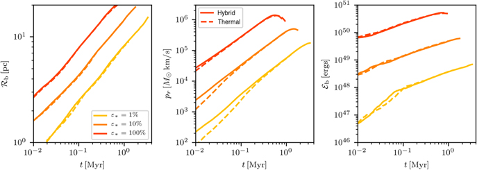
Figure 20. Tests run with purely thermal energy injection, in comparison to the hybrid scheme explained in the main text. All panels are analogous to the top panels shown in Figure 21. Results using the hybrid injection scheme (thermal scheme) are shown with solid (dashed) lines. The evolution of the total radial momentum,  is very slightly delayed for the thermal scheme compared to the hybrid feedback mechanism, but reaches the same scaling by the time the bubble radius is
  .
.
Download figure:
Standard image High-resolution imageB.2. Reduced Mass Loss
For practical reasons, our simulations use a value for the wind mass-loss rate per unit stellar mass,  , that is about a factor of 5 larger than that predicted by the SB99 code for a Kroupa IMF. From Figure 1, this results in a wind momentum injection rate a factor of
  larger than from SB99. To confirm that our theory still applies when using a lower value for
  , we ran tests with
  , similar to the SB99 level. This correspondingly reduces the momentum injection rate to
  . With a lower momentum injection rate, the right-hand side of Equation (14) is reduced, and more cooling (larger Θ) would be required to satisfy the condition for efficient cooling. If this EC condition is not satisfied, energy will build within the bubble, so that the EC predictions for radius, momentum, and energy would underestimate the true values.
For the reduced mass-loss rate, we run three simulations ( , 10%, and 100%) with
  ,
,  , and
, and  . We note that the choice
  (the low-density regime) is the worst case scenario for application of the EC theory since cooling is least efficient at low densities, already making it harder for Equation (14) to be satisfied.
The evolution of the bubble’s effective radius ( ), the total momentum carried by the bubble (
 ) and the total bubble internal energy (
 ) are shown in the top panels of Figure 21. Similar to the figures shown in Section 4, we display the quantities derived from simulations using yellow, orange, and red lines compared to the theoretical predictions of the EC model in black. As expected, the EC theory underestimates
  ,
,  , and
, and  . However, these differences are small, especially in the case of the radial evolution.
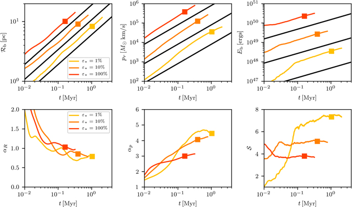
Figure 21. Results of our test runs with smaller mass-loss rates ( ). The top panels show comparisons to the EC theoretical predictions (black) for the bubble’s effective radius (left), total radial momentum (middle), and total energy in the bubble interior (right) for simulations run with
  (yellow), 10% (orange), and 100% (red). The bottom panels show quantities related to the ratio of the simulated and theoretically predicted values (see Section 4.4).
Download figure:
Standard image High-resolution imageMoreover, the temporal dependence of each quantity is still very well described by the EC theory. This is exemplified by the bottom panels of Figure 21, which display quantities related to the ratio of the simulated values to the values predicted by our EC theory. The fact that these quantities are roughly constant and order unity over the course of the simulation, especially for higher-luminosity clusters, reflects that the EC theory still describes evolution reasonably well.
B.3. Changed Feedback Radius
For all the simulations in the main text, we keep the feedback radius, which determines the region where wind energy is injected, constant. As a further test of numerical robustness and convergence, we perform a set of simulations with a feedback radius that is half that given in the main text,  . The set of models is as described in Appendix B.2 but with the normal
  values described in the text and now with
  , so that
  (i.e., the feedback region is still well resolved). We compare to the standard simulations with
  and
and  .
.
The results of the comparison between the  and
and  cases is shown in Figure 22 for the standard quantities of relevance to our theory. As expected, the results for the smaller feedback radius simulations appear to enter the scaling regime earlier than those simulations with larger
  .
.
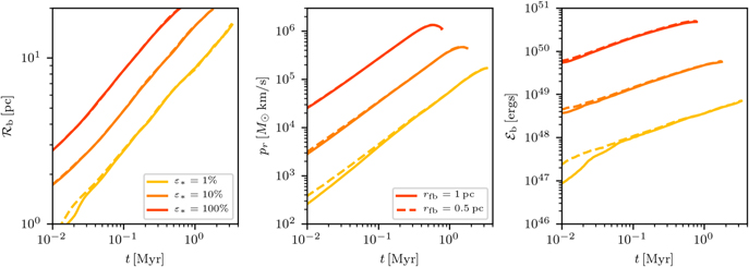
Figure 22. Results of tests with standard ( , solid curve) and and smaller (
 , dashed curve) feedback radius. All panels are analogous to those shown in Figure 20. There is excellent agreement among all quantities, indicating that the changed feedback radius (higher source resolution) does not impact our results.
Download figure:
Standard image High-resolution imageB.4. Different Turbulent Initial Conditions
When initializing the velocity fields in our simulations, we generally use the same set of amplitudes and phases (based on the same sequence of random seeds) to create the turbulent velocity field. With a different initial velocity field (even for the same initial kinetic energy), the background density structure into which the bubble expands would be different. To check whether the results are sensitive to the specific realization of the turbulent velocity field, we perform the same simulations as in Appendix B.2, using the standard  , except we initialize the velocity field with a different random seed.
While the cloud will still have the same statistical density structure, the gas in the immediate vicinity of the star particle will likely be different. We expect this to result in a slightly different early-time evolution of the wind bubble, while the same overall evolution would be followed once the bubble has probed a significant fraction of the cloud size. In reality, the massive stars that create these high-powered winds will preferentially form at density maxima, but such a self-consistent treatment is left for later work.
The results of these tests are shown in Figure 23. So as not to overemphasize the differences at early times, we display these results on a linear (rather than logarithmic) timescale. Comparing to the standard simulation with a different set of turbulent phases, we see that indeed the overall evolution of the wind-driven bubbles is insensitive to the specific density structure within the turbulent cloud.
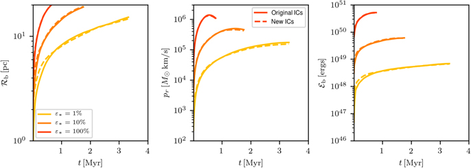
Figure 23. Results of our test runs comparing different initial realizations of the turbulent velocity field, which creates different cloud density structure. All panels are analogous to those shown in Figure 20 except here we use a linear scale for time. This choice is so as to not overemphasize differences in the early evolution, which are due to differences in the density structure very near to the source particle. We show the original initialization as solid lines and the alternate initialization as dashed lines. There is clearly very good agreement at later times between the evolution, in spite of different density structures.
Download figure:
Standard image High-resolution imageAppendix C: Results for Different Mass Clouds
In Table 1 we lay out the full range of simulations that we ran. In the main body of the text we only displayed and discussed results for the cases with  . In this appendix we display results from the runs with cloud masses of Mcloud = 5 × 10⁴ and
  , given in Figures 24 and 25, respectively. Results for both 1283 and 2563 resolution are shown.
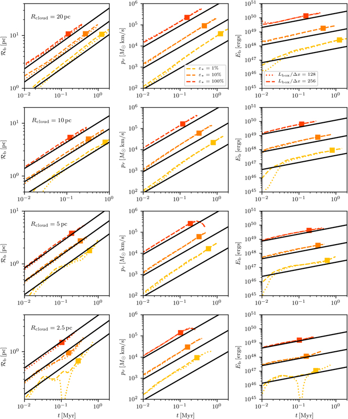
Figure 24. Comparisons of our theory (black curves) to our simulations (colored curves) for cases with cloud mass  and (from top to bottom row) Rcloud = 20, 10, 5, and 2.5 pc. Columns from left to right show the bubble’s effective radius,
  , the total radial momentum,
  , and the total energy in the bubble interior
  . All curves are calculated exactly analogously to those in Figures 4–6.
Download figure:
Standard image High-resolution image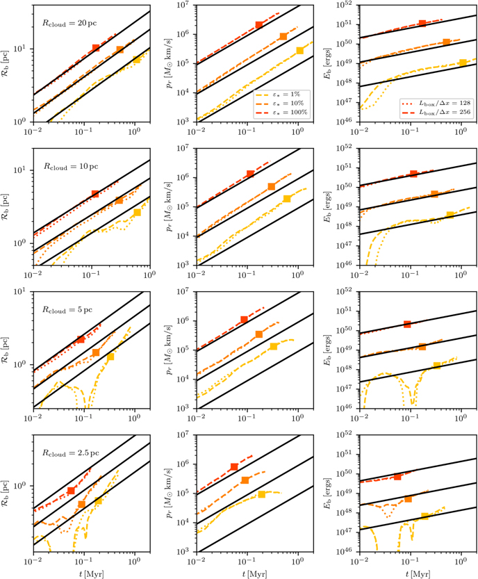
Figure 25. Same as Figure 24 for cases with  .
.
Download figure:
Standard image High-resolution imageFootnotes
- 1
We use the term momentum driven (energy driven) to denote a solution in which momentum (energy) increases linearly in time. The Castor et al. (1975)/Weaver et al. (1977) solution is also internally energy conserving in the sense that there are no radiative energy losses from the hot bubble or its interface with the shell; however, the leading shock is assumed to be fully radiative so that a fraction
of the input wind energy is radiated away as the shocked and accelerated ambient gas cools to join the exterior of the shell. - 2
The measurement technique we adopt was suggested to the authors by Drummond Fielding.
