Abstract
We present the spectral and spatial evolution of H2O masers associated with the water fountain source IRAS 18043−2116, found in observations with the Nobeyama 45 m Telescope and the Australia Telescope Compact Array. We have found new highest-velocity components of the H2O masers (at the redshifted side VLSR ≃ 376 km s−1 and at the blueshifted side VLSR ≃ −165 km s−1), and the resulting velocity spread of ≃540 km s−1 breaks the speed record of fast jets/outflows in this type of sources. The locations of those components have offsets from the axis joining the two major maser clusters, indicating a large opening angle of the outflow (∼60°). The evolution of the maser cluster separation of ∼2.9 mas yr−1 and the compact (∼02) CO emission source mapped with the Atacama Large Millimeter-submillimeter Array suggest a very short (∼30 yr) timescale of the outflow. We also confirmed an increase in the flux density of the 22 GHz continuum source. The properties of the jet and the continuum sources and their possible evolution in the transition to the planetary nebula phase are further discussed.
Original content from this work may be used under the terms of the Creative Commons Attribution 4.0 licence. Any further distribution of this work must maintain attribution to the author(s) and the title of the work, journal citation and DOI.
1. Introduction
Water fountains (WFs) are evolved stars, mostly in the post-asymptotic giant branch (post-AGB) phase that show H2O maser emission tracing high-velocity collimated jets when they are observed at high angular resolution (see Imai 2007 and Desmurs 2012 for reviews). The velocity spread in their H2O maser spectra is typically >50 km s−1, and can be as large as ≃500 km s−1 (Gómez et al. 2011). Their H2O maser emission thus traces significantly faster motions than the typical expansion velocities of circumstellar envelopes (CSEs) during the AGB phase (10–30 km s−1; Sevenster et al. 1997). The WFs identified so far seem to be in the short transition phase between the AGB and the planetary nebula (PN) phases of low-mass stars (initial stellar masses ≲4 M☉; Khouri et al. 2021). The short dynamical ages of the maser jets (5–100 yr; Imai 2007; Tafoya et al. 2020) may indicate that WFs represent one of the first manifestations of collimated mass loss in evolved stars. It is believed that jets carving the CSEs play an essential role in the shaping process of the PNe (Sahai & Trauger 1998; Tafoya et al. 2020). Interestingly, the spatio-kinematics of WFs show a wide variety, from clear collimation and bipolarity to more complicated patterns such as multiple arc-shaped patterns (Orosz et al. 2019), sometimes with additional low-velocity components that may be associated with the relics of slowly expanding circumstellar material, probably ejected during the AGB phase (Imai et al. 2013). A rapid deceleration of a fast WF jet may show up in the systematic velocity drifts of individual peaks in the maser spectrum. One such example is IRAS 18113−2503, in which the jet would have been launched at an initial velocity of 800 km s−1 and decelerated to 200–300 km s−1 within 20–30 yr (Orosz et al. 2019). Such deceleration is also expected for the jet in W43A, with more direct evidence (Tafoya et al. 2020). Thus, single-dish and interferometric observations of H2O masers in these sources are able to trace the evolution of the collimated jet or even measure directly the growth of the WF outflow.
IRAS 18043−2116 (hereafter abbreviated as I18043) was first reported as a WF by Deacon et al. (2007) with H2O maser emission, which covered a velocity range of 210 km s−1 (+185 to −20 km s−1) around the stellar systemic velocity of VLSR ≃ 87.0 km s−1 km s−1 (Deacon et al. 2004). Later, Walsh et al. (2009) reported H2O maser emission over a velocity spread of nearly 400 km s−1 (+289 to −109 km s−1). More recently, Pérez-Sánchez et al. (2017) reported maser emission spread over a more redshifted velocity range from +349 to −46 km s−1. Therefore, this WF may host the second fastest jet identified in the H2O maser spectra just after IRAS 18113−2503 (Gómez et al. 2011). The distance to I18043 is estimated to be ∼11 kpc using the Revised Kinematic Distance Calculator (Reid et al. 2014) on the basis of the systemic velocity of this source (VLSR ≃ 87.0 km s−1, see Section 3.3 for more details). This calculator is based on a Galactic model that is best suited for star-forming regions and, therefore, its application to evolved stars can cause some uncertainty in the estimated distance. However, WFs are located close to the Galactic plane and they are expected to follow the Galactic rotation (Imai et al. 2007). Also, this distance is in good agreement with the value of 8.20 ± 1.75 kpc calculated from modeling the spectral energy distribution of I18043 (Vickers et al. 2015).
Here we present new detections of the highest-velocity components of the masers in I18043 yielded with the 45 m telescope of the Nobeyama Radio Observatory (NRO) and with the Australia Telescope Compact Array (ATCA). These detections broke the record of the top speed of the jet in I18043. We also present the follow-up mapping observations of the H2O masers with ATCA to locate the new maser components. The radio continuum emission associated with I18043 was also mapped. The whole structure of the outflow has been revealed by the observation of CO J = 2 → 1 emission with the Atacama Large Millimeter-submillimeter Array (ALMA).
Section 2 summarizes those NRO, ATCA, and ALMA observations. Section 3 presents the results of the observations. Section 4 provides the discussion on the evolution of the high-velocity jet traced by H2O maser and CO emission. The time variability in the continuum emission, which has also been confirmed in the present work, is also discussed.
2. Observations
2.1. Nobeyama Radio Observatory 45 m Telescope
Single-dish monitoring observations of H2O and SiO masers toward WFs were conducted in the “Finest Legacy Acquisitions of SiO- and H2O-maser Ignitions by the Nobeyama Generation” (FLASHING) survey. FLASHING has been described in detail in Imai et al. (2020) and Amada et al. (2022), including the specification and the record of the observations with the NRO 45 m Telescope since 2018 December. The summary paper of FLASHING will be published in a separate paper. Here we focus on the FLASHING observations of H2O (at the rest frequency of 22.235080 GHz) masers in I18043 conducted during 2019 January–2020 April, including the epochs of the new discovery of the highest-velocity components and those within 1 month of the ATCA observations, described later. Each of the observations lasted for about 1 hr.
We used three spectral windows to obtain a total velocity coverage of ∼1600 km s−1. Each spectral window had 2048 spectral channels, each with a velocity resolution of 0.41 km s−1. Data reduction was carried out using the JavaNewstar package 9 in a standard manner, namely, data integration in the time domain followed by spectral baseline fitting in the maser emission-free spectral channels. We adopt a conversion factor of 2.8 Jy K−1 to convert the antenna temperature to the flux density scale.
2.2. Australia Telescope Compact Array
The ATCA observations presented in this paper were conducted on 2020 April 7 and 30, 2020 June 4, and 2021 March 30 within project C3361, which is a follow-up of the sources monitored in the FLASHING program in order to increase the temporal sampling of spectra, and to obtain information on the evolution of the spatial distribution of the H2O masers. Two independent spectral windows were observed, centered at 18 and 22 GHz, with a bandwidth of 2 GHz each, obtaining full linear polarization products. We set up the Compact Array Broadband Backend in its 64M-32k mode, which samples each of these spectral windows in 32 broadband channels per polarization with a coarse spectral resolution of 64 MHz, for radio continuum observations. Several of the broadband channels were further zoomed in to observe the H2O maser line with a finer spectral resolution of 0.42 km s−1. The total velocity coverage for the line was 1727 km s−1 on April 7 and 3453 km s−1 in the later three sessions.
Initial calibration was carried out using standard procedures in Miriad. The absolute flux density scale was calibrated with the source PKS 1934−638. PKS 0537−441 was also used as a bandpass calibrator for the first epoch, while PKS 1613−586 was used for the other three epochs. The sources IERS B1817−254, PMN J1832−2039, IERS B1817−254, and PMN J1755−2232 were used as complex-gain calibrators in each of the four epochs, respectively. Further processing (imaging, deconvolution, and self-calibration) was carried out with the Astronomical Image Processing System (AIPS). For the continuum data, we flagged out the broadband channels containing the maser line, to avoid contamination. In the line data, the spectral channel with strongest maser emission was used for self-calibration as well as reference position for the maps. The phase and amplitude corrections for self-calibration were obtained at 10 s intervals (the integration time of each individual visibility). These solutions were then applied to both the whole spectral data set and the broadband continuum data centered at 22 GHz. Since the line and continuum data share the same calibration corrections, the 1σ relative positional accuracy among individual maser components and between maser and continuum emission is approximately given by the size of the synthesized beam divided by 2 times the signal-to-noise ratio (S/N) of the emission.
We note that the beam is highly elongated along the north–south direction, which strongly worsens the positional accuracy in that direction. The synthesized beams were 253 × 0
34 at a position angle of −6.78° and 1
42 × 0
41 at a position angle of −1.27° on 2020 April 30 and 2021 March 30, respectively. In these two sessions only, the uv coverage was good enough to map the maser emission while the spectra were obtained for all the four sessions previously mentioned. We roughly estimate a positional accuracy of ∼20 mas (1σ) along the minor axis of the beam (almost in the east–west direction) for a component with an S/N ∼ 10. The relative positions of the maser components with respect to the reference one were determined by Gaussian fitting using the AIPS task JMFIT, assuming a single Gaussian component in each velocity channel. This simple assumption looks valid for distinguishing clusters of the maser components described in Section 3.2.
2.3. Atacama Large Millimeter-submillimeter Array
I18043 was also observed with ALMA on 2019 January 18 (project code: 2018.1.00250.S). The details of these observations are presented by Khouri et al. (2021). The spectral setup covered a frequency range that contains emission of the CO(J = 2 → 1) line at 230.538 GHz. In this paper, we present only the spectrum and image of the CO(J = 2 → 1) in order to estimate the systemic velocity of I18043 and compare the spatio-kinematical distribution of the masers with that of the molecular material. The integration time of ∼11 min yielded an rms noise level of 3 mJy in the spectrum for a velocity resolution of 1.5 km s−1, and a synthesized beam of 124 × 1
18 with a position angle of −78°. The relative position accuracy is ∼60 mas for a component with an S/N ∼ 10.
3. Results
3.1. FLASHING/ATCA Spectra of Masers
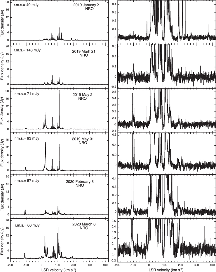
Figure 1 shows a time series of the spectra of H2O masers of I18043 taken with the NRO 45 m telescope and ATCA during 2019 January 2–2021 March 30. Because of the rapid variation in the spectral profile from one observation epoch to another, it is difficult to directly check the consistency of the flux density scales between the spectra of the NRO 45 m telescope and ATCA. However, the maser components around VLSR ∼82 km s−1 had flux densities of ∼4 Jy in both spectra of the two telescopes during 2020 April 7–16, suggesting that the flux density scales are roughly consistent with each other within ∼10%.
Download figure:
Standard image High-resolution image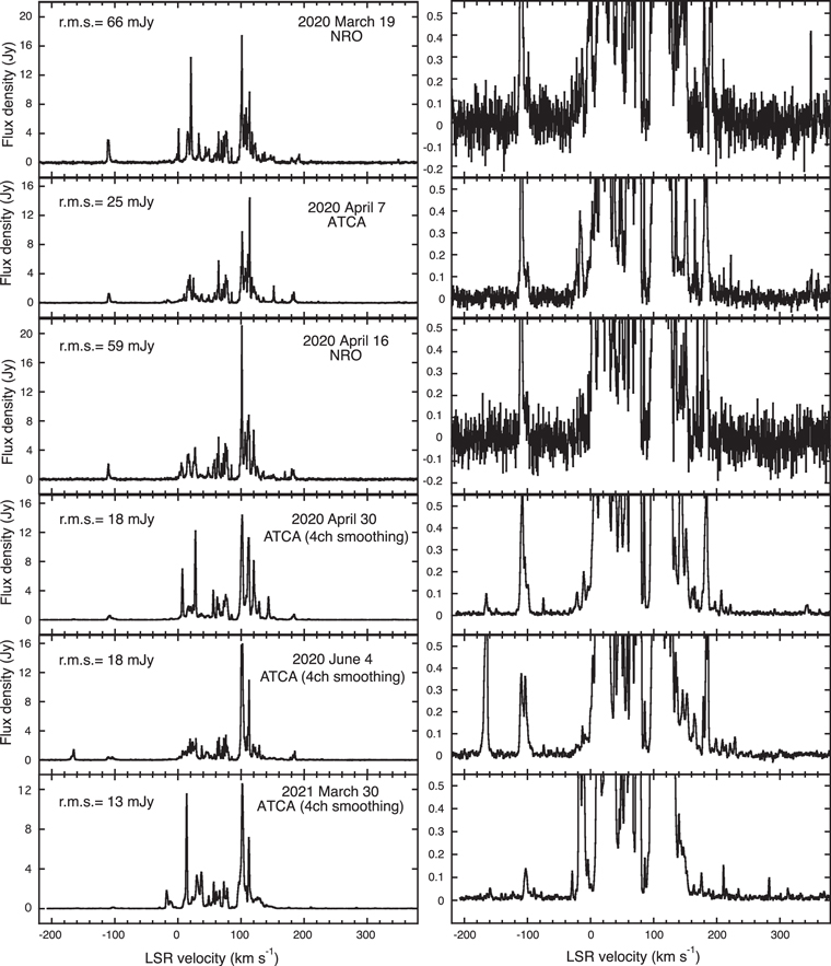
Figure 1. Spectra of H2O masers in I18043 taken with ATCA and NRO telescopes during 2019 January 2–2021 March 30. The rms noise levels are indicated in each spectrum.
Download figure:
Standard image High-resolution imageThe FLASHING session on 2019 January 2 detected the redshifted side of the new velocity components at VLSR ≃ 376 km s−1, while the ATCA session on 2020 April 30 detected the blueshifted side of the new velocity component at VLSR ≃ −165 km s−1. These detections break the record of the velocity spread of the maser components in this source (−100 km s−1 > VLSR > 350 km s−1; Walsh et al. 2009; Pérez-Sánchez et al. 2017); this suggests that the top speed of the jet in I18043 has to be revised. Moreover, this velocity spread (≃540 km s−1) is the largest ever detected in the spectra of H2O masers of WFs, beating the previously reported one for IRAS 18113−2503 (≃500 km s−1; Gómez et al. 2011).
It is difficult to determine whether these extreme velocity components may be decelerating, as suggested by Orosz et al. (2019) for IRAS 18113−2503, due to their too short lifetimes within a few months. However, their seemingly constant velocities within ∼1 km s−1 on this timescale may rule out such rapid deceleration (up to 10 km s−1 month−1).
3.2. ATCA Maps of H2O Masers and the Continuum Source
Figure 2 shows the maps of H2O masers taken in I18043 with ATCA on 2020 April 30 and 2021 March 30. Although some of the maser components have relatively large positional uncertainties (up to 500 mas) in the decl. offset, almost parallel to the elongation direction of the synthesized beam, the maser map resolves the structure of the bipolar outflow in the east–west direction. One can see two main clusters of maser components at (A) −75 ≤ VLSR ≤ 83 km s−1 and (B) 83 ≤ VLSR ≤ 188 km s−1, as well as another blueshifted cluster (C) −113 ≤ VLSR ≤ −98 km s−1. An additional redshifted group (D) 206 ≤ VLSR ≤ 209 km s−1 is also tentatively visible to the west of cluster B. The most redshifted component (VLSR ∼ 344 km s−1) also may be included in the group D while the most blueshifted component (VLSR ∼ −165 km s−1) can be included in the group C, taking into account their positional uncertainties mentioned above.
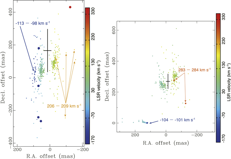
Figure 2. Left: map of H2O masers in I18043 taken with ATCA on 2020 April 30. The maser distribution has a larger positional uncertainty in decl. offset. The scatter of the weak (S/N ≃ 10) blueshifted (VLSR = −113 to −98 km s−1) and the redshifted (VLSR = 206–209 km s−1) components is attributed to such a large positional uncertainty in this direction, but the mean positions of each of the blue- and redshifted components are still close to the major alignment axis of the two major clusters of the masers. The new blueshifted components (VLSR ∼ −165 km s−1) and the redshifted components (VLSR ∼ 344 km s−1) are highlighted in bigger filled circles. The position and the size of the black cross indicate the position and statistical error (3σ) of the continuum source, respectively. The synthesized beam is 253 × 0
34 at a position angle of −6.78°. Right: same as the left panel but on 2021 March 30. The new blueshifted components (VLSR ∼ −102 km s−1) and the redshifted components (VLSR ∼ 284 km s−1) are highlighted in bigger filled circles. The synthesized beam is 1
42 × 0
41 at a position angle of −1.27°.
Download figure:
Standard image High-resolution imageFigure 2 also shows the location of the continuum source (X, Y) = (15 ± 23, 165 ± 131) (mas) on 2020 April 30 and (X, Y) = ( −13 ± 4, 270 ± 16) (mas) on 2021 March 30. The continuum source had a flux density of Sν = 0.75 ± 0.05 mJy on 2020 April 30 and Sν = 0.97 ± 0.09 mJy on 2021 March 30. The location of the continuum source, detected at S/N ≃ 36, also may have a large positional uncertainty related to the synthesized beam shape. Nevertheless, it is clear that the continuum source is located between the blue- and redshifted H2O maser clusters.
These ATCA maps taken in 2020–2021 can be directly compared with Figure 3 of Pérez-Sánchez et al. (2017) taken in 2013. Although it is difficult to quantitatively compare the separations of the maser clusters in a time span of ∼7 yr, one can see that the separation between clusters A and B looks consistent. Taking into account the stellar systemic velocity of VLSR ≃ 87 km s−1 (Deacon et al. 2004), clusters A and B may form a pair with spectral and spatial symmetry with respect to the central star. Regarding the stellar systemic velocity, we revised its value using CO emission detected with ALMA; see Section 3.3.
In the same manner, cluster C and group D will form another symmetric pair. However, cluster C and group D in 2020–2021 have large uncertainties in their locations and distributions. Group D in 2020–2021 may be coincident to cluster B in 2013 (Pérez-Sánchez et al. 2017), while cluster C has been newly visible ∼50 mas east of cluster A.
Figure 3 highlights the maser distributions during 2020–2021 in the east–west direction in which the relative maser positions were better determined. The separation between the two major clusters A and B is discussed in more detail in Section 4.
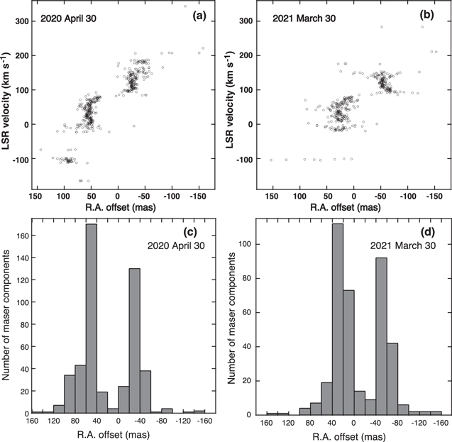
Figure 3. Distribution of H2O masers in I18043 along R.A. offset found with ATCA. (a) LSR velocity distribution of the masers on 2020 April 30. (b) Same as panel a, but on 2021 March 30. (c) Histogram of R.A. offsets on 30 April 2020. (d) Same as panel c, but on 30 March 2021.
Download figure:
Standard image High-resolution image3.3. Atacama Large Millimeter-submillimeter Array Maps of CO Lines
Figure 4 shows the spectrum of the CO(J = 2 → 1) emission observed with ALMA. The line consists of a strong central component and high-velocity wings, which are indicated in the left panel of Figure 4. The high-velocity wings extend over a velocity range >200 km s−1, although the blueshifted wing exhibits contamination of foreground gas that probably belongs to molecular clouds along the line of sight. From the velocity of the line peak of the central component, a systemic velocity of VLSR,sys = 87 ± 1 km s−1 is derived for I18043. This value is compatible with the systemic velocity obtained by Deacon et al. (2004) using OH maser observations.
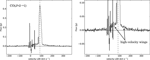
Figure 4. Left: ALMA observations of the CO(J = 2 → 1) emission in I18043. The vertical dashed line indicates the systemic velocity of the source, VLSR,sys = 87 km s−1. Right: zoom in toward the CO(J = 2 → 1) emission around the systemic velocity to show the high-velocity wings.
Download figure:
Standard image High-resolution imageThe spatial distribution of the CO(J = 2 → 1) and 230 GHz continuum emission is shown in Figure 5. There exists an offset of the brightness centroids between the blue- and redshifted components (<02), and the spatially unresolved brightness distributions of these components well support the far distance to this source and the compactness of the jet structure (≲11 kpc × 0
2 ∼2200 au).
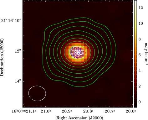
Figure 5. Integrated CO(J = 2 → 1) emission around the systemic velocity of I18043 observed with ALMA. The green contours represent the velocity-integrated emission in the velocity range 65–110 km s−1. The values of the contours are 3 × σ × 1.6n, with n = 0, 1, 2, 3,…, and σ the rms value of the emission, 0.07 Jy beam−1 km s−1. The blue and red contours represent the velocity-integrated emission in the velocity ranges −125–65 km s−1 and 110–300 km s−1, respectively. The values of the contours are 0.7, 0.75, 0.8, 0.85, 0.9, and 0.95 times the peak value of the emission, which is 0.62 Jy beam−1 km s−1 and 1.1 Jy beam−1 km s−1 for the blue- and redshifted emission, respectively. The background image corresponds to the intensity of the CO(J = 2 → 1) emission. See the scale to the right side.
Download figure:
Standard image High-resolution imageThe locus of the CO(J = 2 → 1) emission peak in each bin with a velocity width of 6 km s−1 is presented in Figure 6. There is a clear velocity gradient in R.A. offset with respect to the 230 GHz continuum peak, as shown in the right panel of Figure 6.
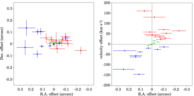
Figure 6. Left: peak positions of the ALMA CO(J = 2 → 1) emission in each bin toward I18043. The position of the 230 GHz continuum is indicated with a black triangle, R.A.(J2000) = 18h07m20851, decl.(J2000) = −21°16
12
13. Right: R.A. offsets from the continuum peak position as a function of the velocity offset from the systemic velocity, VLSR,sys = 87 km s−1. The blue, green, and red marks represent emission in the velocity ranges −170 < Voffset < −20 km s−1, −10 < Voffset < 10 km s−1, and 10 < Voffset < 170 km s−1, respectively. These figures seem to be obtained after averaging two spectral channels in the green velocity range and nine spectral channels in the blue and red velocity ranges.
Download figure:
Standard image High-resolution image4. Discussion
4.1. Characteristics of the Outflow in I18043 from the H2O Maser and CO Line Emissions
We measured the separation between the two main clusters of H2O masers, blue- and redshifted with respect to the systemic velocity ≃87 km s−1. This separation of the two clusters was ∼45 ± 5 mas on 2008 July 12 (Walsh et al. 2009). On the other hand, it has changed to ∼74.1 ± 0.4 mas and 87.6 ± 0.5 mas on 2020 April 30 and 2021 March 30, respectively, as shown in Figure 3. Note that the uncertainties in these separations are statistical. This result may indicate a possible expansion of the cluster separation at a rate of ∼2.9 ± 0.5 mas yr−1, namely a growth of a bipolar outflow hosting the two clusters.
We also note that the angular separations of the red- and blueshifted groups of H2O masers in I18043, ∼74 and 88 mas, correspond to a linear length of ∼800 and 950 au, respectively. They are quite similar to the separation of the red- and blueshifted groups of masers in IRAS 16552−3050 (∼700 ± 100 au; Suárez et al. 2008; Vickers et al. 2015). On the other hand, the velocity spreads are rather different between these two WFs (∼540 and ∼170 km s−1; Suárez et al. 2008). The origin of the difference in the velocity spreads (inclination of the jet major axis, stellar luminosity, evolution phase) will be further investigated.
In a previous analysis of Very Long Baseline Array (VLBA) data from 2008 October 26 and 2009 January 25 in I18043, Orosz (2017) was able to distinguish two distinct arc-shaped groups of masers, blue- and redshifted with respect to the systemic velocity of ∼87 km s−1. The blueshifted maser emission was within a velocity range from −111 km s−1 to 78 km s−1 and the redshifted maser emission was within a velocity range from 94 km s−1 to 176 km s−1. Comparing these results with those by Walsh et al. (2009), it seems that the high-velocity components detected previously at velocities higher than 200 km s−1 were not included in the VLBA epochs, with a velocity coverage up to 227 km s−1 (Day et al. 2011). In our recent observations, we were able to detect higher-velocity components than those previously reported, in both the blue- and redshifted sides of the spectra at velocities up to VLSR ≃ −165 km s−1 and ≃376 km s−1, respectively. This velocity spread is the largest ever detected in a WF ≃540 km s−1. The emergence of the new highest-velocity components at the outer outflow lobes may indicate a rapid growth of the outflow triggered by an increase in the maximum outflow velocity.
From two epochs of the VLBA data, 2008 October 26 to 2009 January 25, Orosz (2017) estimated roughly the expansion rate of the outflow to be ∼1 mas yr−1, with an average separation of the two maser clusters of ∼63 mas. If we extrapolate the expansion rate of the outflow from 2009 to 2020, the separation of the two clusters would be ∼74 mas, which is consistent with the results of the ATCA observations. Thus, the dynamical age of the outflow is estimated to be tjet ≲ 30 yr, using the expansion rate and the separation of the two clusters from the VLBA data. Orosz (2017) used the full velocity spread of the H2O masers seen in their VLBA maps (+176 to −111 km s−1) and derived the inclination angle of the jet’s major axis to be ijet ∼ 75° with respect to the plane of the sky. Using this inclination angle, we estimate a 3D expansion velocity for the redshifted side of Vjet,3D ∼ 170 or 300 km s−1, when assuming mean proper motions of ∼1 and 2.9 mas yr−1, respectively, considering the most redshifted components observed with ATCA of VLSR ∼ 284 and 344 km s−1, respectively.
The CO(J = 2 → 1) emission consists of a spatially extended low-velocity component, shown as green contours in Figure 5, and a compact high-velocity component, shown as blue and red contours. The green contours represent the velocity-integrated emission in the velocity range +65 to +110 km s−1, and the blue and red contours represent the velocity-integrated emission in the velocity ranges −125 to +65 km s−1 and +110 to +300 km s−1, respectively. The peaks of the blue- and redshifted components have an offset in the east–west direction by approximately 02, with the blueshifted emission located toward the east. Thus, the velocity gradient seen in the CO emission is in agreement with the velocity gradient of the blue- and redshifted masers.
The right panel of Figure 6 shows the locus of the CO(J = 2 → 1) emission peak in each bin with a velocity width of 6 km s−1. The observed dispersion of the locus in the R.A. offset indicates a wide angle of the outflow. We note that there exists a clear velocity gradient in the R.A. offset of the CO emission from −20 to 20 km s−1 with respect to the systemic velocity. This velocity gradient is roughly followed by the blue- and redshifted CO emission, considering the uncertainties and a S/N of 10.
The wanders of the peak positions in the blue- and redshifted CO emission components, Voffset > 70 km s−1, may be affected by the large positional uncertainty, while those in the range Voffset = 10–70 km s−1 are roughly consistent with the ones of H2O masers. This suggests that the H2O masers are associated with the CO outflow itself, or possibly shock regions in the outflow. The absence of CO emission at the fastest velocity range ∣Voffset∣ > 100 km s−1, where the H2O masers are visible, is different from the case of W43A in which the H2O masers are associated with the slower-moving entrained material rather than the faster jet (Tafoya et al. 2020). The CO velocity wanders also indicate a large opening angle of the outflow, within which the locations of different velocity components are scattered due to an inhomogeneity of the outflow velocity. Taking into account the direction coverage of the wandering-velocity components with respect to the originating point of the outflow, the full opening angle of the outflow is estimated to be ∼60°.
Also looking at the right panel of Figure 2 in more detail, the blueshifted components at VLSR ∼ −104 to −101 km s−1 present an offset from the two major clusters of masers A and B. This separation also may imply the presence of a wide-angle outflow, indeed supported by the CO(J = 2 → 1) observations.
Figure 7 shows a schematic picture of the WF I18043, including the current observational panorama discussed in the previous sections. The continuum emission, close to the central stellar system, may correspond to an ionized area at the inner part of a biconical outflow. Farther away from the central system, around several hundreds of au, thick biconical cavities surrounding the outflow are expected from the observed clusters of H2O masers, which are likely excited in the cavities by shock interaction with the outflow. The blue- and redshifted H2O masers may be more amplified along the front and rear sides of the inner cavities, where a longer amplification path is expected close to the line of sight. Moreover, the CO emission is tracing an envelope of several thousands of au. The velocity wanders in the blue- and redshifted components of the CO emission indicate a large opening angle of the biconical outflow (a full angle of ∼60° in each component). This is also consistent with a large scatter of the maser distribution in the direction perpendicular to the major axis of the outflow.
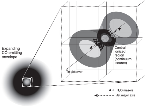
Figure 7. Schematic picture of the system of I18043. The whole expanding envelope (bottom-left corner) is traced in the 65–110 km s−1 component of the CO emission (see Figure 5). The envelope exhibits weak bipolarity in the east–west direction, indicated by a velocity gradient (see Figure 6). The center of the envelope is ionized (either by photons from the central star or by shocks at the outflow), as indicated by the 22 GHz continuum emission (see Figure 2). This part is zoomed in on the right side, exhibiting a biconical outflow. The distribution of H2O masers (black and gray circles for the blue- and redshifted components, respectively) exhibits strong bipolarity in the present ATCA (see Figure 2) and VLBA (Orosz 2017) data.
Download figure:
Standard image High-resolution imageApart from the H2O maser emission detected at 22 GHz, this source also presents H2O maser emission at 321 GHz. These maser components span a velocity range similar to that at 22 GHz, indicating that these H2O masers at both frequency transitions probably coexist. The intensity of the submillimeter masers is comparable to that of the 22 GHz masers, implying the kinetic temperature of the region where the submillimeter masers originate is Tk > 1000 K (Tafoya et al. 2018).
4.2. Characteristics of the Radio Continuum Emission in I18043
The origin of the radio continuum emission in this source is also relevant to understand its evolution. Pérez-Sánchez et al. (2017) obtained flux density data at four frequency bands between 1.5 and 22 GHz. They reported spectral indices (α, defined as Sν ∝ να ) < 2 between 1.5 and 5.5 GHz. Specifically, we estimated a value of 0.49 ± 0.09 from their data between 1.5 and 5.5 GHz, and α = −0.2 ± 0.2 between 5.5 and 22 GHz. These values are consistent with free–free radiation from a plasma, which ranges from α = 2 (optically thick regime) to −0.1 (optically thin), with an optical depth decreasing at higher frequencies. As mentioned by these authors, the spectral indices should be taken with care, since these observations were not simultaneous: the data at 22 GHz were taken in 2015, two years after those at lower frequencies, and the radio continuum emission in evolved stars is known to be variable (Cerrigone et al. 2011). Pérez-Sánchez et al. (2017) argued that if the radio continuum emission happened to fade with time, then the flux density at 22 GHz at the time of the low-frequency observations (2015) would have been lower, leading to a spectral index at high frequencies significantly lower than −0.1, which in its turn would point out to a nonthermal contribution. Actually, a decreasing flux density has been suggested in itself as being a signature of nonthermal radio continuum emission (Suárez et al. 2015; Cerrigone et al. 2017). However, following this line of reasoning, our data at 22 GHz do not show any evidence for a nonthermal component, since the radio continuum emission at 22 GHz seems to be consistently increasing: while a flux density of 0.70 ± 0.10 in 2013 July was obtained by Pérez-Sánchez et al. (2017), we measured Sν = 0.75 ± 0.05 mJy on 2020 April 30 and Sν = 0.97 ± 0.09 mJy on 2021 March 30. This is a factor 1.3 increase in one year in our observations, with an apparently higher increase rate in our observations than in the previous ones by Pérez-Sánchez et al. (2017).
Considering, then, that the current radio continuum data are compatible with thermal free–free emission from electrons in a plasma, we note that the spectral index α = 0.49 ± 0.09 in the Pérez-Sánchez et al. (2017) data between 1.5 and 5.5 GHz indicates a partially optically thick emission. It is also close to the standard value of ne ∝ r−2 expected in the case of an isotropic distribution of electrons with a radial variation of electron density of ne ∝ r−2, where r is the distance to the central star (Olnon 1975; Panagia & Felli 1975). This would be the case of an isotropic ionized wind or a photoionized region at the beginning of the PN phase (since the previously ejected envelope would also have an r−2 density dependence). Under the assumption of an isotropic wind, Pérez-Sánchez et al. (2017) obtained a mass-loss rate of ≃3 × 10⁻⁵ (D/11 kpc) M⊙ yr−1.
However, I18043 clearly shows the presence of a collimated jet traced by H2O maser emission, therefore assuming an isotropic ionized wind may not be appropriate. In this sense, Pérez-Sánchez et al. (2017) mentioned that the mass-loss rate they obtained under this assumption is an upper limit to the actual value. On the other hand, a collimated, ionized jet with ne
∝ r−2 would also show a similar spectral index in its radio continuum emission (Reynolds 1986), with a particular value depending on the jet geometry. In this model, a biconical jet (constant opening angle) would give α = 0.6, while lower or higher values correspond to a jet whose width decreases or increases with distance from the star, respectively. Here the jet half-width is given by w ∝ r
, where
is related to the spectral index as α = 1.3–0.7/
following Reynold’s model. The case of a standard spherical wind yields
= 1 and α = 0.6. On the other hand, an isothermal, constant-velocity, fully ionized flow yields 0.5 <
≤ 1 and 0.6 ≥ α > −0.1. For the case of I18043, α = 0.49 and
≃ 0.89, therefore the radio continuum emission is congruous with a fully ionized collimated outflow.
In an ionized jet, the flux density of the radio continuum emission can provide an estimate of the mass-loss rate. Using Equation (8) in Anglada et al. (2018) and the parameters from the jet traced by H2O masers, we estimate  M⊙ yr−1 and ≃6 × 10⁻⁶
M⊙ yr−1, considering the flux density at 5.5 GHz and the spectral index α = 0.49 measured by Pérez-Sánchez et al. (2017) in 2013, and a jet velocity of 170 and 300 km s−1, respectively. In this calculation we assumed an injection opening angle of the jet equal to 60°, a distance to the source of 11 kpc, an electron temperature of 104 K, an inclination angle 75° with respect to the plane of the sky, and a turnover frequency of ≃5.5 GHz. On the other hand, we obtain the following values for the mass-loss rates from 2 to 4 × 10⁻⁶
M⊙ yr−1 when they are derived from the flux density measurements at 22 GHz in 2020−2021, although these are likely to be lower limits, considering that the continuum emission at this frequency may be in the optically thin regime (Pérez-Sánchez et al. 2017). This would suggest that, if the continuum emission arises from a jet, its mass loss is increasing. In any case, better estimation of the physical parameters would require an up-to-date measurement of the continuum spectrum of the source, with (nearly) simultaneous observations at a wide range of frequencies. Even so, these values of the mass-loss rates are not very accurate; they seem to be higher than those expected in models of post-AGB stars (≃10−7–10−8
M⊙ yr−1; Vassiliadis & Wood 1994), although these models follow the evolution of a single star. Lately, observations and models suggest that the presence of collimated jets in WFs could be due to a binary system in the center, leading to the formation of accretion disks from which the collimated outflow can be launched. In particular, these objects seem to have gone through a common-envelope phase (García-Segura et al. 2021; Khouri et al. 2021), which greatly enhances mass-loss rates.
M⊙ yr−1 and ≃6 × 10⁻⁶
M⊙ yr−1, considering the flux density at 5.5 GHz and the spectral index α = 0.49 measured by Pérez-Sánchez et al. (2017) in 2013, and a jet velocity of 170 and 300 km s−1, respectively. In this calculation we assumed an injection opening angle of the jet equal to 60°, a distance to the source of 11 kpc, an electron temperature of 104 K, an inclination angle 75° with respect to the plane of the sky, and a turnover frequency of ≃5.5 GHz. On the other hand, we obtain the following values for the mass-loss rates from 2 to 4 × 10⁻⁶
M⊙ yr−1 when they are derived from the flux density measurements at 22 GHz in 2020−2021, although these are likely to be lower limits, considering that the continuum emission at this frequency may be in the optically thin regime (Pérez-Sánchez et al. 2017). This would suggest that, if the continuum emission arises from a jet, its mass loss is increasing. In any case, better estimation of the physical parameters would require an up-to-date measurement of the continuum spectrum of the source, with (nearly) simultaneous observations at a wide range of frequencies. Even so, these values of the mass-loss rates are not very accurate; they seem to be higher than those expected in models of post-AGB stars (≃10−7–10−8
M⊙ yr−1; Vassiliadis & Wood 1994), although these models follow the evolution of a single star. Lately, observations and models suggest that the presence of collimated jets in WFs could be due to a binary system in the center, leading to the formation of accretion disks from which the collimated outflow can be launched. In particular, these objects seem to have gone through a common-envelope phase (García-Segura et al. 2021; Khouri et al. 2021), which greatly enhances mass-loss rates.
An alternative explanation for the origin of the radio continuum emission is the onset of photoionization at which this source is entering the PN phase. An increase in the flux density at radio wavelengths has also been observed in several young PNe (Kwok et al. 1981; Knapp et al. 1995; Christianto & Seaquist 1998; Gómez et al. 2005; Tafoya et al. 2009; Cala et al. 2022). Such a flux density increase has been interpreted as an expansion of the ionized region. If this is the case, then an increase by a factor of 1.3 in flux density would correspond to an expansion by a factor of 1.14 in radius in one year for an isotropic ionized region. We should consider that the size of the emitting region is unresolved in our observations, therefore we are not able to estimate other physical parameters such as the mass of the ionized region. Furthermore, the scenario of a photoionized region around this source has also been discussed by Pérez-Sánchez et al. (2017), but they concluded that a shock-ionized wind is more likely to explain the observed radio continuum emission. Whether it is a shock- or radiative-ionized region around I18043, further observations would be necessary to identify the actual scenario.
5. Summary
The spectral and spatial evolution of the H2O masers in I18043 observed with the Nobeyama 45 m Telescope and ATCA reveal new highest-velocity components located at the outer outflow lobes (up to ∼950 au), suggesting a rapid growth of the outflow triggered by an increase in the maximum outflow velocity. This source presents the largest velocity spread ever detected in the spectra of H2O masers of a WF ≃540 km s−1. The spatial distribution of the H2O masers may indicate the presence of an outflow with a large opening angle ∼60° and a very short timescale ∼30 yr.
The Nobeyama 45 m radio telescope is operated by Nobeyama Radio Observatory, a branch of the National Astronomical Observatory of Japan (NAOJ), National Institutes of Natural Sciences. The Australia Telescope Compact Array is part of the Australia Telescope National Facility (grid.421683.a), which is funded by the Australian Government for operation as a National Facility managed by CSIRO. We are thankful to the referee for his/her useful comments that helped us to improve this paper. L.U. acknowledges support from the University of Guanajuato (Mexico) grant No. CIIC 090/2023. H.I. and G.O. are supported by the JSPS KAKENHI grant No. JP16H02167. J.F.G. acknowledges support from grant Nos. PID2020-114461GB-I00 and CEX2021-001131-S, funded by MCIN/AEI/10.13039/50110001103. H.I. and J.F.G. were supported by the Invitation Program for Foreign Researchers of the Japan Society for Promotion of Science (JSPS grant No. S14128). D.T. was supported by the ERC consolidator grant No. 614264. G.O. was supported by the Australian Research Council Discovery project DP180101061 of the Australian government, and the grants of CAS LCWR 2018-XBQNXZ-B-021 and the National Key R&D Program of China grant No. 2018YFA0404602.
Facilities: Nobeyama 45 m Telescope - , ATCA - , ALMA. -
Footnotes
- *
Released on 2021 March 1.
- 9