Abstract
We consider if outflowing winds that are detected via narrow absorption lines (NALs) with FWHM of <500 km s−1 (i.e., NAL outflows) in quasar spectra contribute to feedback. As our sample, we choose 11 NAL systems in eight optically luminous quasars from the NAL survey of T. Misawa et al. (2007a), based on the following selection criteria: (i) they exhibit “partial coverage” suggesting quasar origin (i.e., intrinsic NALs), (ii) they have at least one low-ionization absorption line (C ii and/or Si ii), and (iii) the Lyα absorption line is covered by available spectra. The results depend critically on this selection method, which has caveats and uncertainties associated with it, as we discuss in a dedicated section of this paper. Using the column density ratio of the excited and ground states of C ii and Si ii, we place upper limits on the electron density as ne < 0.2–18 cm−3 and lower limits on their radial distance from the flux source R as greater than several hundreds of kpc. We also calculate lower limits on the mass outflow rate and kinetic luminosity of  1.9–5.5 and
  –49.8, respectively. Taking the NAL selection and these results at face value, the inferred feedback efficiency can be comparable to or even larger than those of broad absorption line and other outflow classes, and large enough to generate significant active galactic nucleus feedback. However, the question of the connection of quasar-driven outflows to NAL absorbers at large distances from the central engine remains open and should be addressed by future theoretical work.
Original content from this work may be used under the terms of the Creative Commons Attribution 4.0 licence. Any further distribution of this work must maintain attribution to the author(s) and the title of the work, journal citation and DOI.
1. Introduction
Outflowing winds from active galactic nuclei (AGN) deposit energy and momentum into the interstellar medium (ISM) and circumgalactic medium and regulate the star formation activity of their host galaxies. This could contribute significantly to the evolution of the host galaxies (i.e., AGN feedback; J. Silk & M. J. Rees 1998; E. Scannapieco & S. P. Oh 2004; E. Choi et al. 2018) if the total kinetic luminosity of the outflowing winds is larger than ∼0.5% (P. F. Hopkins & M. Elvis 2010) or ∼5% (E. Scannapieco & S. P. Oh 2004; T. Di Matteo et al. 2005) of the quasar’s Eddington luminosity.
AGN outflowing winds are often found via broad absorption lines (BALs) with line widths of ≥2000 km s−1 in the spectra of about 15%–40% of optically selected quasars (e.g., R. J. Weymann et al. 1991; X. Dai et al. 2008; C. Knigge et al. 2008; R. R. Gibson et al. 2009; J. T. Allen et al. 2011). Their ejection velocities from the quasars (vej) range from several hundred up to 30,000 km s−1 or more (R. J. Weymann et al. 1991; F. Hamann et al. 2018; P. Rodríguez Hidalgo et al. 2020).
Powerful outflows of several quasars with BALs (i.e., BAL quasars) have kinetic luminosities that satisfy the above feedback conditions (e.g., N. Arav et al. 2013; B. C. J. Borguet et al. 2013; X. Xu et al. 2019; H. Choi et al. 2020; D. Byun et al. 2022a; A. Walker et al. 2022). Significant feedback is especially likely for extremely high-velocity outflows with outflow velocities of ∼0.1c–0.2c (e.g., P. Rodríguez Hidalgo et al. 2020; G. Vietri et al. 2022), similar to the ultrafast outflows that are often detected via absorption lines in the X-ray spectra of AGNs (F. Tombesi et al. 2010; J. Gofford et al. 2013).
In addition to BALs, narrow absorption lines (NALs) with line widths of ≤500 km s−1 and their intermediate subclass (mini-BALs) with line widths of 500–2000 km s−1 have been used to study AGN outflowing winds (T. Misawa et al. 2007a; D. Nestor et al. 2008; F. Hamann et al. 2011; R. Ganguly et al. 2013; C. Culliton et al. 2019; M. Dehghanian et al. 2024). A substantial fraction of NALs found in quasar spectra do not arise in gas that are physically related to the quasars themselves (intervening NALs, hereafter); they arise in cosmologically intervening absorbers such as foreground galaxies, the intergalactic medium, and Milky Way gas. But some fraction of NALs have been associated with quasar outflows (intrinsic NALs, hereafter) based partly on the following statistical arguments: (1) the detection rate of NALs varies depending on the physical properties of the background quasars (e.g., optical and radio luminosity, radio spectral index, and radio morphology; G. T. Richards et al. 1999; G. T. Richards 2001) and (2) a significant fraction of NALs remains after accounting for the contributions from cosmologically intervening absorbers and absorbers associated with quasar host galaxies or their cluster environment (D. Nestor et al. 2008; V. Wild et al. 2008). Additional arguments for such an association include time variability, partial coverage, or line-locking exhibited by some NALs (F. Hamann et al. 1997b; T. R. Lewis & D. Chelouche 2023). However, identifying specific intrinsic NALs is not straightforward because they do not display all the traits of other intrinsic absorption systems, such as BALs and mini-BALs, at the same time. Some NALs do vary (a fraction of ∼20%–25%; e.g., D. Narayanan et al. 2004; J. H. Wise et al. 2004) and some display partial coverage (e.g., T. Misawa et al. 2007a). NALs that do display partial coverage do not do so in all the transitions from the same system. Therefore, the selection of samples of intrinsic NALs has some inherent ambiguity and any sample selected by these criteria may be contaminated by intervening NALs (we return to these issues in Section 3 and discuss how they affect the work presented here). In view of the properties described just above, any NALs that may be intrinsic are unlikely to be associated with the same portions/regions of quasar outflows that produce BALs and mini-BALs (e.g., R. Ganguly et al. 2001, associated the NAL gas with different layers of the outflow than the BAL gas; alternatively, the NAL gas may be at a different distance from the central engine than the BAL gas). Moreover, the structure of NAL absorbers is likely to be different from the structure of BAL and mini-BAL absorbers; in fact, NAL absorbers have been suggested to be filaments with an inner, low-ionization “core” surrounded by an outer, tenuous, higher-ionization layer (e.g., C. Culliton et al. 2019) in order to explain the detection of partial coverage in only some transitions from the same system.
There are two possible interpretations of the fraction of quasars hosting BALs, NALs, and mini-BALs. The first is an orientation scenario, in which BALs are observed if our line of sight (LoS) to the continuum source passes through the main, dense stream of the outflowing wind (e.g., M. Elvis 2000; R. Ganguly et al. 2001; F. Hamann et al. 2012). In this scenario, the difference in line width could depend the inclination angle of our LoS relative to the outflow direction or on the distance of the gas producing the different absorption lines from the continuum source. The latter possibility is bolstered by the association of blueshifted absorption lines with outflowing gas at a wide range of distances from the continuum source, from parsecs to hundreds of kilo-parsecs (e.g., M. de Kool et al. 2001; C. Chamberlain et al. 2015; D. Itoh et al. 2020). An alternative idea is the evolution scenario, in which BAL quasars are in an evolutionary stage (e.g., just after galaxy merging) in which they are obscured by dust (S. L. Lípari & R. J. Terlevich 2006; D. Farrah et al. 2007). This scenario is supported by the observation that the BAL quasar fraction, outflow velocity, and line width of absorption lines at zabs ≥ 6 are a few times larger than those at lower redshift (M. Bischetti et al. 2022, 2023).
The physical parameters of outflowing winds have been studied through variability of the strengths and profiles of the absorption lines, since almost all BALs and mini-BALs vary over a few years in the quasar’s rest frame (e.g., R. R. Gibson et al. 2008; D. M. Capellupo et al. 2012; T. Misawa et al. 2014). The probability of variation increases with the time interval between observations, approaching unity for intervals of a few years (D. M. Capellupo et al. 2013). When multiple BAL troughs are present, they often tend to vary in a coordinated fashion (e.g., N. Filiz Ak et al. 2013; Z. S. Hemler et al. 2019). In extreme cases, BAL profiles appear or disappear (e.g., N. Filiz Ak et al. 2012; S. M. McGraw et al. 2017; Sameer et al. 2019). Possible origins of such variations include (a) motion of the absorbing gas parcels across our LoS and (b) changes in the ionization state of the absorber (e.g., T. Misawa et al. 2007b; F. Hamann et al. 2008; J. A. Rogerson et al. 2016; H.-Y. Huang et al. 2019; G. Vietri et al. 2022).
In past studies, the mass flow rate ( ) and kinetic luminosity (
 ) of outflowing winds have been estimated as follows: (1) the electron number density (ne) is determined using measurements of troughs from excited states (e.g., F. W. Hamann et al. 2001; B. C. J. Borguet et al. 2012), or from the variability timescale of BALs and mini-BALs (e.g., F. Hamann et al. 1997a; T. Misawa et al. 2005), (2) the ionization parameter (U) and total Hydrogen column density (NH) are determined by comparing the observed column densities of various ions to simulated values using photoionization models (e.g., X. Xu et al. 2018; T. R. Miller et al. 2020a; A. Walker et al. 2022), (3) the radial distance of the absorber from the center (R) is then obtained from the values of ne and U (e.g., D. Narayanan et al. 2004; J. A. Rogerson et al. 2016), and (4) the knowledge of R, NH and the velocity of the outflow (vej) allows us to determine the mass flow rate (
 ) and kinetic luminosity (
 ) of a given outflow (see Sections 3 and 4 for details).
While the feedback efficiency of BALs and mini-BALs have been studied in detail, those of NALs have hardly been examined because most NALs are so stable that we cannot extract information from time-variability analysis. However, NALs potentially have large values of  (∝vej) and
  (∝
(∝ ) and could contribute significantly to AGN feedback since they appear to be more common (∼50%) and have larger outflow velocities (up to ∼0.2c) compared to BALs and mini-BALs (T. Misawa et al. 2007a).
In recent years,  and
and  of AGN outflows have been evaluated using absorption lines from ground states (i.e., resonance lines) and excited states of ions such as C ii, Si ii, O iv, and Ne v (e.g., N. Arav et al. 2018; D. Byun et al. 2022a, 2024). This method has two advantages over time-variability analysis: (i) it requires only a single-epoch spectrum and (ii) it can be applied to absorption lines that do not vary, such as NALs.
In this study, we investigate the feedback efficiency of quasars using intrinsic NAL absorbers, in contrast to past studies that focused on BALs and mini-BALs. We select intrinsic NAL candidates using their partial coverage signature, which is subject to caveats. We calculate the physical parameters using excited and ground state absorption lines instead of time-variability analysis. We describe the sample selection in Section 2 and discuss its caveats in Section 3. We present the analysis in Section 4, and our results and discussion in Section 5. Finally, Section 6 summarizes our work. Throughout this paper, we use a cosmology with H0 = 69.6 km s−1 Mpc−1, Ωm = 0.286, and ΩΛ = 0.714 (C. L. Bennett et al. 2014).
2. Sample Selection
In this work, we rely on partial coverage analysis to select quasars with intrinsic NALs. This selection method involves several caveats, which we discuss in Section 3 but it is the only method that can yield a sample of quasars with available high-resolution spectra suited for the analysis that we carry out here. T. Misawa et al. (2007a) identified 39 intrinsic NAL candidates based on partial coverage analysis of C iv, N v, and Si iv doublets in the spectra of 20 bright quasars at zem = 2–4. Since the original sample included 37 quasars, at least 50% of quasars host intrinsic NALs. The detection limits in rest-frame equivalent width were  (C iv) = 0.056 Å,
  (N v) = 0.038 Å, and
  (Si iv) = 0.054 Å.
The quasars were originally selected for a survey aimed at measuring the Deuterium-to-Hydrogen abundance ratio (D/H) in the Lyα forest (e.g., S. Burles & D. Tytler 1998a, 1998b). Therefore, the target selection does not have a direct bias with respect to the properties of any intrinsic absorption-line systems, although there could be indirect bias since the sample contains only optically bright quasars. The observations were carried out with Keck/HIRES with a slit width of 1 14 (i.e., FWHM ∼ 8 km s−1). The spectra were extracted with the automated program, MAKEE, written by Tom Barlow.
We focus on 16 intrinsic NAL candidates of the 39 absorption systems that have at least one low-ionization absorption line from an ion with ionization potential between 13 and 24 eV (e.g., O i, Si ii, Al ii, and C ii). We reject two systems with large column densities of  > 19 since there are several observational indicators suggesting that some (sub-)DLAs,4
contain small-sized and high-density clouds within themselves: e.g., occurrence of time variation (T. L. Hacker et al. 2013) and emergence of absorption lines from ions in excited states (e.g., A. M. Wolfe et al. 2003).
> 19 since there are several observational indicators suggesting that some (sub-)DLAs,4
contain small-sized and high-density clouds within themselves: e.g., occurrence of time variation (T. L. Hacker et al. 2013) and emergence of absorption lines from ions in excited states (e.g., A. M. Wolfe et al. 2003).
Of the remaining 14 systems, we choose 11 systems in eight quasars as our sample because (i) they have C ii and/or Si ii NALs which are necessary for the excited/resonance line analysis, and (ii) the Lyα absorption line of the system is covered by past observations which is necessary for measuring total column densities of the outflowing winds.
We use the software package minfit (C. W. Churchill 1997; C. W. Churchill et al. 2003) to fit absorption lines with Voigt profiles using the absorption redshift (zabs), column density ( in cm−2), Doppler parameter (b in km s−1), and covering factor (Cf) as free parameters.
The covering factor, Cf, is the fraction of photons from the background flux source that pass through the foreground absorber along our LoS; it is a measure of the dilution of the depths of absorption lines and needs to be included to get the correct column density. We evaluate Cf as
where Rb and Rr are the residual fluxes at the blue and red members of a doublet in the normalized spectrum (e.g., E. J. Wampler et al. 1995; T. A. Barlow & W. L. W. Sargent 1997; F. Hamann et al. 1997a). If Cf < 1, the absorbers are likely arising in quasar outflowing winds (i.e., intrinsic absorbers) because cosmologically intervening absorbers such as the CGM of foreground galaxies and the IGM have sizes much larger than the quasar continuum source. Based on the results of the covering factor analysis, T. Misawa et al. (2007a) separated all NALs into three classes: classes A and B were deemed to include reliable and possible intrinsic NALs and class C was taken to include intervening or unclassified NALs. The detailed classification criteria of each class are summarized in T. Misawa et al. (2007a).
The properties of the quasars in our sample are summarized in Table 1. Columns (1) and (2) are the quasar name and emission redshift (zem). Columns (3) and (4) give the V- and R-band magnitudes (mV and mR, respectively). Columns (5)–(8) list the radio-loudness parameter ( ), the bolometric luminosity (Lbol), the mass of the quasar’s supermassive black hole (MBH), and the Eddington luminosity (LEdd). We calculate the bolometric luminosity by Lbol = 4.4λLλ(1450 Å) (see G. T. Richards et al. 2006). We use Sloan Digital Sky Survey spectra to measure the monochromatic luminosity at 1450 Å except for HS1946+7658, for which we use the spectrum of H.-J. Hagen et al. (1992). All spectra are corrected for Galactic extinction (E. F. Schlafly & D. P. Finkbeiner 2011; J. A. Cardelli et al. 1989) before measuring the observed flux. We estimate the BH mass from the FWHM of the C iv emission line, the C iv emission line blueshift relative to the systemic redshift, and λLλ(1350 Å) using the empirical relation of L. Coatman et al. (2017).
Table 1. Sample Quasars
| (1) | (2) | (3) | (4) | (5) | (6) | (7) | (8) |
|---|---|---|---|---|---|---|---|
| Quasar | zem | mVa | mRa |
 b
b
| Lbolc | MBHd | LEdde |
| (mag) | (mag) | (erg s−1) | (M⊙) | (erg s−1) | |||
| Q0805+0441 | 2.88 | 18.16 | ⋯ | 3115 | 1.74 × 1047 | 1.94
| 2.45
|
| HS1103+6416 | 2.191 | 15.42 | ⋯ | <0.62 | 1.18 × 1048 | 2.36
| 2.97
|
| Q1107+4847 | 3.000 | 16.60 | ⋯ | <1.95 | 1.24 × 1048 | 3.30
| 4.16
|
| Q1330+0108 | 3.510 | ⋯ | 18.56 | <16.2 | 3.93 × 1047 | 1.69
| 2.13
|
| Q1548+0917 | 2.749 | 18.00 | ⋯ | <6.96 | 4.20 × 1047 | 5.96
| 7.51
|
| Q1554+3749 | 2.664 | 18.19 | ⋯ | <21.9 | 3.26 × 1047 | 3.54
| 4.46
|
| HS1700+6416 | 2.722 | 16.12 | ⋯ | <1.24 | 2.09 × 1048 | 2.59
| 3.27
|
| HS1946+7658 | 3.051 | 16.20 | ⋯ | <1.35 | 2.87 × 1048 | 8.93
| 1.12
|
Notes. aObserved V- or R-band magnitude from T. Misawa et al. (2007a). bRadio loudness parameter  (5 GHz)/fν(4400 Å) from T. Misawa et al. (2007a). cBolometric luminosity. See discussion in Section 2. dBlack hole mass. See discussion in Section 2. eEddington luminosity.
Download table as: ASCIITypeset image
Table 2 gives the parameters of intrinsic NALs: column (1) gives the quasar name, column (2) the absorption redshift (zabs), column (3) the neutral Hydrogen column density ( ), columns (4)–(6) the ion of the targeted absorption line (C ii or Si ii), and the corresponding column densities in the ground and excited states (
 and
and  ), columns (7) and (8) the derived limit on the electron density (ne) and radial distance from the center (R), and column (9) the reliability class of the intrinsic NAL.
Table 2. Properties of NAL Outflows
| (1) | (2) | (3) | (4) | (5) | (6) | (7) | (8) | (9) |
|---|---|---|---|---|---|---|---|---|
| Quasar | zabs |
 a
a
| IONb |
 c
c
|
 c
c
| ned | Re | Classf |
| (cm−2) | (cm−2) | (cm−2) | (cm−3) | (kpc) | ||||
| Q0805+0441 | 2.6517 | 15.11 | C ii | 13.25 | <12.90 | <14.38 | >108 | A |
| HS1103+6416 | 1.8919 | 15.53 | Si ii | 13.45 | <11.78 | <18.37 | >248 | B |
| Q1107+4847 | 2.7243 | 15.50 | C ii | 12.70 | <12.26 | <11.09 | >328 | A |
| Q1330+0108 | 3.1148 | 14.99 | C ii | 12.52 | <12.07 | <10.78 | >187 | A |
| Q1548+0917 | 2.6082 | 18.00 | C ii | 13.47 | <12.31 | <1.79 | >475 | B |
| 2.6659 | 15.26 | C ii | 13.11 | <12.46 | <6.30 | >253 | A | |
| 2.6998 | 15.70 | C ii | 12.67 | <12.24 | <11.41 | >188 | A | |
| Q1554+3749 | 2.3777 | 15.63 | C ii | 13.38 | <12.33 | <2.33 | >367 | A |
| HS1700+6416 | 2.4330 | 18.33 | C ii | 12.88 | <12.02 | <3.90 | >717 | B |
| HS1946+7658 | 2.8928 | 17.11 | C ii | 12.34 | <11.71 | <6.64 | >644 | A |
| 3.0497 | 17.37 | C ii | 13.44 | <11.35 | <0.20 | >3712 | A |
Notes. aColumn density of neutral Hydrogen. bIon for which the column density, electron density, and absorber’s radial distance are reported in columns (5)–(8). cColumn densities of the ion in column (4) in the ground and excited states. dElectron density of the ion in column (4). eAbsorber’s radial distance, corresponding to the ion listed in column (4). fNAL classification made in T. Misawa et al. (2007a).
Download table as: ASCIITypeset image
3. Caveats Associated with the Sample Selection
The conclusions of this work depend critically on whether the NALs that we have selected are indeed intrinsic. As we noted in Section 1, NALs do not show all the properties that signal the association of BALs and mini-BALs with an outflowing wind. Therefore, we highlight here the uncertainties associated with the partial coverage analysis method that is the basis of our selection.
- 1.It is possible that compact, dense clouds in a low-ionization state can exist in over-dense regions in DLA and sub-DLA systems. This possibility is suggested by (a) studies that find variable NALs at large blueshifts from the quasars toward which they are observed (see T. L. Hacker et al. 2013), (b) NALs from low-ionization, dense clouds that may show partial coverage in a handful of DLA or sub-DLA systems5 (see T. M. Jones et al. 2010), and by a variety of models for the ISM of galaxies that predict compact, low-ionization clouds (e.g., D. Pfenniger & F. Combes 1994; A. M. Wolfe et al. 2003; S. C. O. Glover & M.-M. Mac Low 2007; A. Fujita et al. 2009). Such clouds could have sizes of a few astronomical units and exhibit partial coverage, although our targets that exhibit partial coverage in higher-ionized species (i.e., C iv and Si iv) are likely to have larger sizes.
- 2.Intrinsic NALs that are identified based on partial coverage (Cf < 1) do not show any other evidence connecting them to intrinsic absorbers (e.g., time variability and broad line width) as seen in BALs and mini-BALs. Therefore, we cannot corroborate that they are intrinsic by an additional and separate test.
- 3.Intrinsic NALs have a black (i.e., fully absorbed) Lyα trough (Cf = 1) while BAL and mini-BAL systems show a nonblack Lyα trough (Cf < 1). Moreover, in most cases only one component in the intrinsic NAL systems we have selected shows Cf < 1, while the other components are consistent with Cf = 1.
To guard against the first caveat, we exclude DLA and sub-DLA systems from our sample, even if they show partial coverage. The second and third caveats introduce uncertainty in our selection of intrinsic NALs since we have to rely only on the partial coverage signature from one transition. Nonetheless, we do note that (a) photoionization models for intervening absorbers that can produce C iv and Si iv lines typically have kpc-scale sizes (e.g., J. Stern et al. 2016; Sameer et al. 2024), and (b) intrinsic absorbers may have a dense, compact core that can produce partial coverage in some transitions and a more extended halo that can produce full coverage in others (see C. Culliton et al. 2019).
4. Analysis
We calculate the mass outflow rate ( ), kinetic luminosity (
 ), and eventually the feedback efficiency following the prescription of B. C. J. Borguet et al. (2012). First, we need to estimate the absorber’s radial distance from the ionizing continuum source (R), total Hydrogen column density (NH), and ejection velocity (vej). Of these parameters, only vej is measured directly from the observed spectra.
We estimate the absorber’s distance R based on the definition of the ionization parameter6

where Q(H) is the total number of Hydrogen ionizing photons emitted per unit time, nH is the Hydrogen number density, and c is the speed of light. In order to evaluate accurately the ionization parameter, it is necessary to use photoionization models. However, the number of absorption lines detected in these NAL systems is limited to only three elements (i.e., H, C, and Si) and the covering factor of single lines (i.e., Lyα, C ii, and Si ii) cannot be evaluated in practice, which prevents us from constraining the photoionization models effectively. Therefore, we instead assume  = −2.6 because that is the ionization state where the average value of the column density ratio7
of C ii and C iv in our NAL systems, N(C ii)/N(C iv) ∼ 0.3, is approximately reproduced (F. Hamann 1997).8
We convert the quasar bolometric luminosity Lbol to Q(H) using a conventional quasar SED that is a segmented power law, fν ∝ ν−α, where α = 0.4, 1.6, and 0.9 at
= −2.6 because that is the ionization state where the average value of the column density ratio7
of C ii and C iv in our NAL systems, N(C ii)/N(C iv) ∼ 0.3, is approximately reproduced (F. Hamann 1997).8
We convert the quasar bolometric luminosity Lbol to Q(H) using a conventional quasar SED that is a segmented power law, fν ∝ ν−α, where α = 0.4, 1.6, and 0.9 at  = 13.5–15.5, 15.5–17.5, and 17.5–19.5 Hz, respectively (D. Narayanan et al. 2004).
We also need to know the absorber’s Hydrogen number density nH, which is related to the absorber’s electron density ne as ne ∼ 1.2nH in highly ionized plasma (D. E. Osterbrock & G. J. Ferland 2006). While D. Narayanan et al. (2004) used the variability timescale as an upper limit on the recombination time to estimate the electron density, we use the column density ratio of excited and ground states of C ii and Si ii following previous works (e.g., N. Arav et al. 2013; D. Byun et al. 2022a) since (i) we have spectra from only a single epoch, and (ii) intrinsic NALs are rarely variable (T. Misawa et al. 2014).
We estimate the total Hydrogen column density (i.e., NH I + NH II) from the neutral Hydrogen column density (NH I) using a Cloudy photoionization model (version c17.02, G. J. Ferland et al. 2017) with an ionization parameter of  = −2.6 and the conventional quasar SED as introduced above.
We also use the Voigt profile fitting code minfit to measure column densities as well as Doppler b parameters of ground and excited states of C ii and Si ii. We assume full coverage (i.e., Cf = 1) because we cannot evaluate Cf for single lines. If Cf < 1, our estimate, which assumes Cf = 1, is a lower limit on the column density. However, the estimated electron density ratio Nl/Nu and the corresponding electron density would be insensitive to Cf unless the lines are saturated, as demonstrated in Figure 1. If the absorption lines require multiple components to fit their profiles, we only consider the strongest components for calculating electron densities. Using the column density ratio of the strongest components, we place constraints on the electron density using
where ncr is the critical density, Nl and Nu are the column densities of the ground and excited states, gl and gu are their statistical weights (gu/gl = 2 for the relevant energy levels of C ii and Si ii), ΔE is the energy difference between ground and excited states, k is the Boltzmann constant, and T is gas temperature.
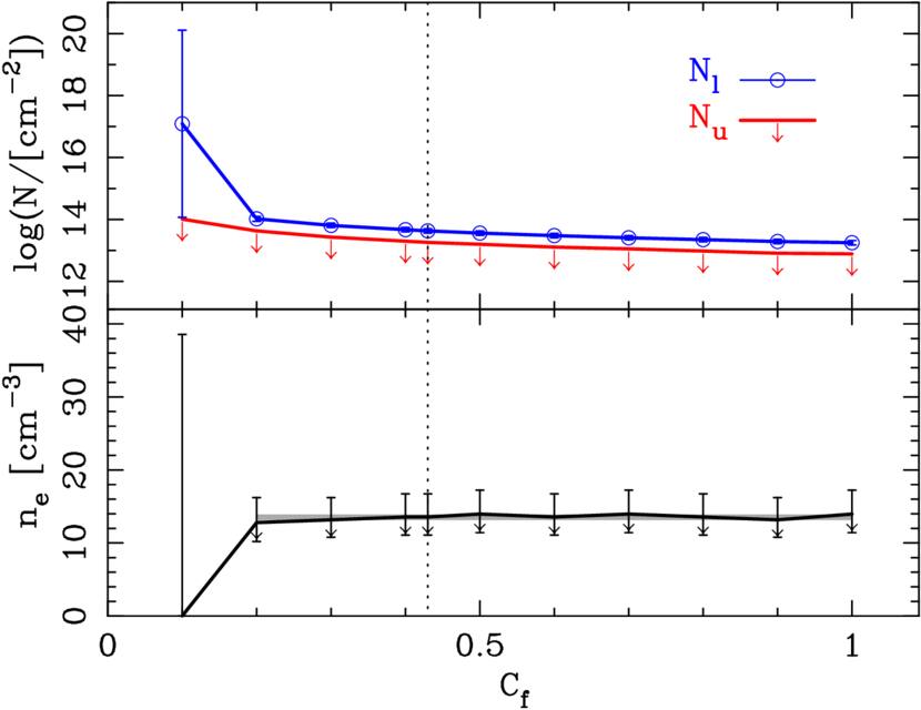
Figure 1. Estimated column densities of the ground and excited states (Nl and Nu, respectively) of the C ii line at zabs = 2.6517 in the spectrum of Q0805+0441 (top panel) and their corresponding electron density (bottom panel) as an example demonstrating the lack of sensitivity of ne to Cf. The C iv line of the system has covering factor of Cf = 0.43 (marked with a vertical dotted line), but the C ii line could have different Cf value. Therefore, we estimate column densities of C ii and C ii* as a function of covering factor. We place only upper limits on N(C ii*) and ne. For Cf ≥ 0.2, an upper limit of ne is almost constant (≤13.5 ± 0.4 cm-3, considering only systematic errors) as shown with the shaded area on the bottom panel.
Download figure:
Standard image High-resolution imageSince ΔE (1.26 × 10⁻¹⁴ erg and 5.69 × 10⁻¹⁴ erg for C ii and Si ii9 ) is much smaller than kT corresponding to the typical temperature of NAL systems (i.e., T ∼ 104 K), the exponential part of Equation (3) can be considered as ∼1. Using the critical densities of C ii and Si ii (ncr ∼ 50 cm−3 and ∼1700 cm−3 for C ii and Si ii; S. S. Tayal 2008a, 2008b), we can calculate the electron densities of the NAL systems.
We place only upper limits on the electron density, which we plot in Figure 2, since (i) no lines in excited states (i.e., C ii*1336, Si ii*1265, Si ii*1533) are detected while the corresponding lines in ground states are detected at a ≥3σ level (see Figure 3 as an example) and (ii) the column densities of ground states are lower limits as described above. Similarly, we place lower limits on the NAL outflow radial distances using Equation (3) of D. Narayanan et al. (2004; see also our Equation (2)). If both C ii and Si ii lines are detected in a single NAL system, we prioritize the former because C ii provides a stronger constraint. In addition to the low-ionization lines, we also evaluate line parameters of neutral Hydrogen (H i) using only the Lyα line.10
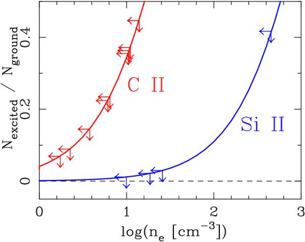
Figure 2. Column density ratios between excited and ground states of C ii and Si ii (red and blue curves) as a function of electron density, which is calculated with the CHIANTI 10.0 Database (K. P. Dere et al. 1997; G. Del Zanna et al. 2021) assuming a gas temperature of 10,000 K. Arrows denote upper limits on the column density ratio of C ii* to C ii and Si ii* to Si ii and the corresponding upper limits on electron density.
Download figure:
Standard image High-resolution image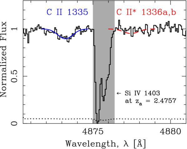
Figure 3. Normalized flux spectrum (solid histogram) and error spectrum (dotted histogram) around the absorption lines of C ii 1335 and C ii* 1336a,b at zabs = 2.6517 in Q0805+0441. The former is detected at a 3σ level, while the latter is not detected. The blue solid curve is a fitted model to C ii 1335. The red dashed curve is a 1σ upper limit on C ii* 1336a,b. The strong absorption profile in the gray shaded area is an unrelated Si iv 1403 line at zabs = 2.4757.
Download figure:
Standard image High-resolution imageThe column densities of H i, C ii, and Si ii in ground and excited states (only upper limits at 1σ level), electron densities, and radial distances from the quasar continuum source of the 11 NAL absorbers are summarized in Table 2.
5. Results and Discussion
Using the parameters we evaluated in Section 4, we calculate the mass outflow rate and the kinetic luminosity following B. C. J. Borguet et al. (2012):


where fc is the global covering fraction of the NAL outflow, μ (=1.4) is the mean molecular weight, and mp is the proton mass. We use fc = 0.5 since intrinsic NALs are identified in at least 50% of optically luminous quasars (T. Misawa et al. 2007a). Since fc was estimated based only on partial coverage analysis, we caution that it is uncertain. The kinetic luminosity and feedback efficiency estimated below are proportional to fc, therefore they would carry the same fractional uncertainty as fc. By substituting parameters in Table 2 into Equations (4) and (5), we evaluate  and
and  and summarize the results in Table 3.
Table 3. Feedback Efficiency of NAL Outflows
| (1) | (2) | (3) | (4) | (5) | (6) | (7) |
|---|---|---|---|---|---|---|
| Quasar | zabs |
 a
a
| vej |
 b
b
|
 c
c
| εkd |
| (cm−2) | (km s−1) | (M⊙ yr−1) | (erg s−1) | |||
| Q0805+0441 | 2.6517 | 17.75 | 18171 | >7.9 × 101 | >8.24 × 1045 | >0.043 |
| HS1103+6416 | 1.8919 | 18.17 | 29437 | >7.8 × 10² | >2.12 × 1047 | >0.091 |
| Q1107+4847 | 2.7243 | 18.14 | 21385 | >6.9 × 10² | >1.00 × 1047 | >0.047 |
| Q1330+0108 | 3.1148 | 17.62 | 27433 | >1.5 × 10² | >3.65 × 1046 | >0.19 |
| Q1548+0917 | 2.6082 | 20.33 | 11480 | >8.4 × 10⁴ | >3.48 × 1048 | >7.8 |
| 2.6659 | 17.90 | 6727 | >9.7 × 101 | >1.39 × 1045 | >3.1 × 10⁻³ | |
| 2.6998 | 18.34 | 3959 | >1.2 × 10² | >5.78 × 1044 | >1.3 × 10⁻³ | |
| Q1554+3749 | 2.3777 | 18.27 | 24356 | >1.2 × 10³ | >2.23 × 1047 | >0.34 |
| HS1700+6416 | 2.4330 | 20.40 | 24195 | >3.1 × 10⁵ | >5.78 × 1049 | >22 |
| HS1946+7658 | 2.8928 | 19.80 | 11942 | >3.5 × 10⁴ | >1.57 × 1048 | >0.34 |
| 3.0497 | 20.01 | 98 | >2.7 × 10³ | >8.10 × 1042 | >1.8 × 10⁻⁶ |
Notes. aTotal Hydrogen column density including both neutral and ionized Hydrogen. bMass outflow rate. cKinetic luminosity. dFeedback efficiency, defined as the ratio of the NAL kinetic luminosity of the outflow to the Eddington luminosity of the quasar,  . The values in this column assume the absorber distances in Table 2.
Download table as: ASCIITypeset image
The AGN feedback efficiency εk is computed as
where LEdd is the Eddington luminosity, G is the gravitational constant, MBH is the mass of the SMBH, and σT is the Thomson cross section. The feedback efficiencies of the 11 NAL systems in the eight quasars of this study are summarized in Table 3 and plotted in Figure 4.
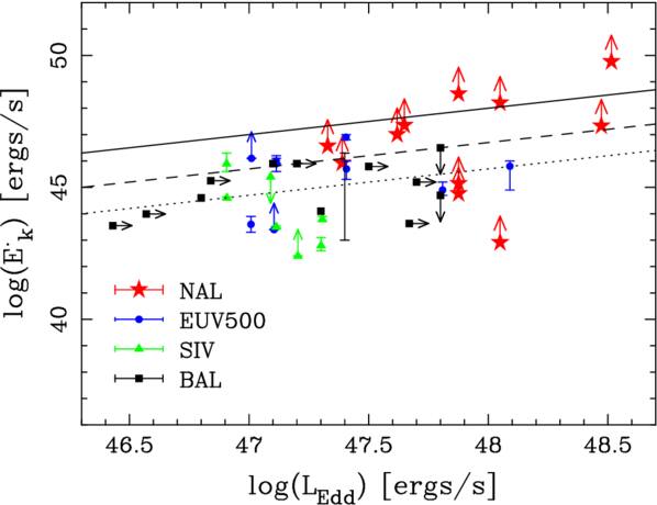
Figure 4. Kinetic luminosity ( ) as a function of the Eddington luminosity (LEdd) for the 11 NAL systems of this study (red), along with nine EUV500 (blue) and seven S iv (green) systems from T. R. Miller et al. (2020b). Filled black squares denote BALs from the literature (D. M. Capellupo et al. 2014; F. Fiore et al. 2017; K. M. Leighly et al. 2018; T. R. Miller et al. 2020a; X. Xu et al. 2020; G. Vietri et al. 2022). Upper limits (rather than lower limits) on
  are given for some S iv and BAL systems since they exhibit time variation. Thick, dashed, and dotted black lines are relations between
  and LEdd for a feedback efficiency of 1, 0.05, and 0.005, respectively.
Download figure:
Standard image High-resolution imageWe emphasize that the mass outflow rate,  , the kinetic luminosity,
  , and the AGN feedback efficiency, εk, reported above are lower limits for the following reasons: (i) Equations (4) and (5) provide lower limits on
  and
and  if outflows are instantaneous (not continuous) with volume filling factors of fV < 1 (see Section 5 of B. C. J. Borguet et al. 2012) and (ii) the radial distances of the absorbers, R, listed in Table 2 are lower limits since we obtain only upper limits on the electron density ne without detecting any C ii and Si ii lines in excited states.
Eight of the 11 NAL systems have lower limits of the feedback efficiency that are large enough to cause significant AGN feedback (i.e., εk > 0.005). Among them, the systems at zabs = 2.6082 in Q1548+0917 and at zabs = 2.4330 in HS1700+6416 have extremely large feedback efficiencies greater than 7, which is due to their relatively large Hydrogen column densities (i.e.,  > 20.3). In contrast, those at zabs = 2.6659 and 2.6998 in Q1548+0917 and at zabs = 3.0497 in HS1946+7658 have relatively small feedback efficiencies. The lower limits on εk of these systems are smaller than 0.005, which is mainly a result of their small ejection velocities (i.e., vej < 7000 km s−1).
We also compare our result to past studies whose targets are (i) BALs (D. M. Capellupo et al. 2014; F. Fiore et al. 2017; K. M. Leighly et al. 2018; T. R. Miller et al. 2020a; X. Xu et al. 2020; G. Vietri et al. 2022), (ii) highly ionized S iv outflows whose ionization potential (IP) is 47.3 eV (T. R. Miller et al. 2020b), and very high-ionized outflows hosting ions with IP of more than 100 eV (e.g., Ne viii, Na ix, and Mg x) whose rest-frame absorption wavelengths are in the extreme-UV region between 500 and 1050 Å (EUV500; T. R. Miller et al. 2020b). As shown in Figure 4, NAL outflows have an exceptionally large efficiency compared to the other outflow classes.
Before closing this discussion, we would like to emphasize that the radial distances of NAL outflows we derived in Section 4 (from about 100 kpc and up to 4 Mpc) are much larger than the typical distances of BAL and mini-BAL outflows. The distances of BAL and mini-BAL outflows have been estimated based on (i) time-variability analysis, (ii) photoionization modeling, and (iii) excited/resonance line analysis similar to that employed in this study, and are found to range from (sub-)parsec (D. M. Capellupo et al. 2014; K. M. Leighly et al. 2018; X. Xu et al. 2020) to tens of kilo-parsecs (F. W. Hamann et al. 2001; D. Byun et al. 2022a, 2022b; A. Walker et al. 2022). In contrast, since NALs are generally not observed to vary (T. Misawa et al. 2014), the radial distances of NAL outflows have been constrained using only the last two of the above methods. Thus, NAL outflows in nearby Seyfert galaxies are found to be located at distances of several to ∼10 kpc from the central engine (e.g., J. P. Dunn et al. 2010; B. C. J. Borguet et al. 2012). Estimates of the distances of NAL outflows in high-z quasars vary significantly. For example, photoionization modeling has suggested a wide range of distances from pc to several kpc for NAL absorbers (even in the same quasar; J. Wu et al. 2010) while methods similar to those used here have suggested distances greater than ∼100 kpc (D. Itoh et al. 2020). Our results here imply even larger radial distances of that absorbing gas (i.e., several hundreds of kpc), which place the NAL outflows away from the immediate vicinity of the quasar central engine and in the outskirts of the host galaxy or in the CGM (see C.-A. Faucher-Giguère et al. 2012; D. Itoh et al. 2020). The small filaments that produce the NALs may result from the interaction of a quasar-launched blast wave with dense gas in the host galaxy, as suggested by C.-A. Faucher-Giguère et al. (2012). These large distances raise the question of the connection between fast, outflowing absorbers to the quasar central engine. Future work should examine whether the NAL outflowing winds indeed have traveled such a long distance from the quasar’s innermost regions to the scale of CGM and IGM, if NALs originate in compact parcels of gas expelled from the quasar host galaxies by quasar-driven outflows, and if other NALs “without” low-ionized species have a different origin (i.e., a different radial distance from the flux source).
6. Summary and Conclusions
In this study, we investigate the physical conditions of NAL outflows to test whether they contribute to AGN feedback. We carefully choose 11 NAL systems in eight quasars from T. Misawa et al. (2007a), and search for excited lines of C ii and Si ii ions to place constraints on their electron densities and radial distances from the continuum source. Although no lines from excited states are detected, we place lower limits on the mass outflow rates, kinetic luminosities, and feedback efficiencies of NAL outflows for the first time. Our main results are as follows:
- 1.We study 11 NAL systems that were identified as intrinsic based on partial coverage analysis. We reiterate here that the selection method has caveats and uncertainties associated with it, which we discuss in Section 3. We also note that because the properties of intrinsic NALs are different from those of BALs and mini-BALs, the corresponding absorbers are probably associated with a different part or phase of the quasar outflow.
- 2.The outflows traced by intrinsic NALs have large mass ejection rates, kinetic luminosities, and feedback efficiencies, namely
 1.9–5.5, –49.8, and εk ≳ 0–22.
 - 3.Eight of the 11 cases studied here have feedback efficiencies greater than 0.5% (P. F. Hopkins & M. Elvis 2010), implying that they contribute significantly to AGN feedback.
- 4.The feedback efficiency of some NAL outflows is larger than those of other outflow classes including BALs, high-ionized S iv, and very high-ionized EUV500 outflows. Such high efficiencies suggest that the outflows traced by NALs could deliver significant feedback from the quasar to the host galaxy.
- 5.The radial distances of NAL outflows are estimated to be very large (i.e., hundreds of kilo-parsecs), which is larger than the typical distance of BAL outflows of 1 pc–10 kpc. This result raises the question of what is the connection of the outflows traced by NALs to the quasar central engine? Do intrinsic NALs trace the portion of the outflow that has already left the quasar host galaxy? This connection has to be understood before we can fully evaluate how the NAL gas fits into the bigger picture of quasar-driven outflows.
- 6.Taking these results at face value, we conclude that we need to take NAL outflows into account for estimating AGN feedback efficiency. However, additional work is needed to confirm the connection of NALs with partial coverage to quasar-driven outflows and to corroborate the results presented here.

For further investigation, we should obtain UV spectra of our sample quasars to detect a number of metal absorption lines (both from the ground states and excited states) in NAL systems, and place more stringent constraints on their electron densities and radial distances.
Our sample consists of only luminous quasars with bolometric luminosity of  47.2, which could bias the results in two ways: (i) luminous quasars have larger outflow velocity, mass outflow rate, kinetic luminosity, and feedback efficiency (R. Ganguly & M. S. Brotherton 2008; F. Fiore et al. 2017; G. Bruni et al. 2019), and (ii) luminous quasars over-ionize the CGM and the IGM around them, both in the LoS (S. Bajtlik et al. 1988; J. Scott et al. 2000) and transverse (J. X. Prochaska et al. 2013; P. Jalan et al. 2019; T. Misawa et al. 2022) directions. By observing a number of fainter quasars to increase the sample size, we will be able to study quasar feedback more generally. Moreover, we will increase the chances of detecting C ii and Si ii NALs in their excited states, which will help us get a more detailed understanding of the feedback efficiency of NAL outflows.
Acknowledgments
We would like to thank the anonymous referee for their comments, which helped us improve this paper. We also would like to thank Christopher Churchill for providing us with the minfit software packages. This work was supported by JSPS KAKENHI grant No. 25K01038.
The data presented herein were obtained at the W. M. Keck Observatory, which is operated as a scientific partnership among the California Institute of Technology, the University of California and the National Aeronautics and Space Administration. The Observatory was made possible by the generous financial support of the W. M. Keck Foundation. The authors wish to recognize and acknowledge the very significant cultural role and reverence that the summit of Maunakea has always had within the indigenous Hawaiian community. We are most fortunate to have the opportunity to conduct observations from this mountain.
Funding for the Sloan Digital Sky Survey (SDSS)-IV has been provided by the Alfred P. Sloan Foundation, the U.S. Department of Energy Office of Science, and the Participating Institutions. SDSS-IV acknowledges support and resources from the Center for High Performance Computing at the University of Utah. The SDSS website is www.sdss.org.
SDSS-IV is managed by the Astrophysical Research Consortium for the participating institutions of the SDSS Collaboration, including the Brazilian Participation Group, the Carnegie Institution for Science, Carnegie Mellon University, Center for Astrophysics ∣ Harvard & Smithsonian, the Chilean Participation Group, the French Participation Group, Instituto de Astrofìsica de Canarias, The Johns Hopkins University, Kavli Institute for the Physics and Mathematics of the Universe (IPMU)/University of Tokyo, the Korean Participation Group, Lawrence Berkeley National Laboratory, Leibniz Institut für Astrophysik Potsdam (AIP), Max-Planck-Institut für Astronomie (MPIA Heidelberg), Max-Planck-Institut für Astrophysik (MPA Garching), Max-Planck-Institut für Extraterrestrische Physik (MPE), National Astronomical Observatories of China, New Mexico State University, New York University, University of Notre Dame, Observatário Nacional/MCTI, The Ohio State University, Pennsylvania State University, Shanghai Astronomical Observatory, United Kingdom Participation Group, Universidad Nacional Autónoma de México, University of Arizona, University of Colorado Boulder, University of Oxford, University of Portsmouth, University of Utah, University of Virginia, University of Washington, University of Wisconsin, Vanderbilt University, and Yale University.
Footnotes
- 4
Damped Lyα systems.
- 5
These systems also suffer from unresolved saturation, but photoionization models identify them as extremely dense and cold absorbers corresponding to the molecular gas in the Milky Way.
- 6
The ionization parameter is defined as U ≡ nγ/nH, where nγ is ionizing photon density.
- 7
The column densities of C ii and C iv are evaluated by fitting Voigt profiles to their absorption troughs. We evaluate a column density of C ii using the same covering factor as C iv. We also assume C ii and C iv absorbers have same ionization parameter in a single-phase, since their absorption profiles are very similar with negligible velocity offset from each other.
- 8
We also perform photoionization models ourselves for an optically thin cloud with solar abundance assuming a conventional quasar SED (D. Narayanan et al. 2004) and confirm that the ionization condition of
= −2.6 well reproduces the column density ratio of N(C ii)/N(C iv) ∼ 0.3. - 9
- 10
Although higher order Lyman series lines (e.g., Lyβ) are covered by some spectra of our sample quasars, their corresponding signal-to-noise ratio is very low.
