Abstract
Xu & Jing reported a monotonic relationship between the host halo mass Mh and the morphology of massive central galaxies, characterized by the Sérsic index n, at fixed stellar mass, suggesting that morphology could serve as a good secondary proxy for the halo mass. Since their results were derived using the indirect abundance matching method, we further investigate the connection between the halo properties and central galaxy morphology using weak gravitational lensing. We apply galaxy–galaxy lensing to measure the excess surface density around CMASS central galaxies with stellar masses in the range of  , using the Hyper Suprime-Cam shear catalog processed through the Fourier_Quad pipeline. By dividing the sample based on n, we confirm a positive correlation between n and Mh, and observe possible evidence of the positive correlation of n and halo concentration. After accounting for color, we find that neither color nor morphology alone can determine the halo mass, suggesting that a combination of both may serve as a better secondary proxy. In comparison to hydrodynamic simulations, we find that TNG300 produces much weaker correlations between Mh and n. Furthermore, using SIMBA simulations with different feedback modes, we find that jet-mode active galactic nuclei feedback might be related to the relationship between the Sérsic index and halo mass.
Original content from this work may be used under the terms of the Creative Commons Attribution 4.0 licence. Any further distribution of this work must maintain attribution to the author(s) and the title of the work, journal citation and DOI.
1. Introduction
In the ΛCDM cosmological model, the large-scale structure of the Universe is shaped by the gravitational influence of dark matter, such as halos, filaments, and voids. These dark matter halos subsequently act as “seeds” for galaxy formation. Dark matter, a substance that has not yet been directly observed, constitutes the major mass of the Universe, whereas stars are the luminous objects we can observe. The stellar-to-halo mass relation (SHMR) reveals the intimate connection between the stellar mass of galaxies and the mass of dark matter halos, indicating the link between galaxy formation and the evolution of dark matter halos. It is generally believed that massive dark matter halos host more massive galaxies. Therefore, by utilizing SHMR, we can assign galaxy masses to halos in N-body simulations or infer halo mass from stellar mass. This allows for a deeper understanding of the evolutionary history of galaxies and their coevolution with dark matter halos.
Although SHMR provides critical insights into the connection between galaxies and halos, it also exhibits significant scatter (M. C. Cooper et al. 2010; A. R. Zentner et al. 2014; Y. Zu et al. 2021, 2022; K. Xu et al. 2023), potentially correlated with the influence of other galaxy properties such as size, color, and morphology. For instance, some studies find that the halos of blue (star-forming) galaxies are less massive than those of red (quenched/passive) galaxies with the same stellar mass (A. Rodríguez-Puebla et al. 2015; R. Mandelbaum et al. 2016; E. N. Taylor et al. 2020; W. Wang et al. 2021; K. Xu & Y. Jing 2022). Conversely, other studies (J. L. Tinker et al. 2013; B. P. Moster et al. 2018; H. Guo et al. 2019) report the opposite conclusion.
The morphology of galaxies is also found to correlate with the halo mass. The galaxy morphology is typically described by the Sérsic profile (J. Sérsic 1963), which characterizes the brightness, size, and morphology of a galaxy. The Sérsic profile is modeled as:
where bn is defined through γ(2n;bn) = Γ(2n), and Γ and γ are the Gamma function and the lower incomplete Gamma function, respectively. Ie is the surface brightness at the half-light radius Re. The Sérsic index n quantifies the curvature of the galaxy’s luminosity profile, with higher values indicating a more concentrated core of light distributions. In this work, we focus on the relation between the halo mass and morphology of galaxies, characterized by the Sérsic index (n). Studies from A. Sonnenfeld et al. (2019) utilize lensing data from the Hyper Suprime-Cam Survey (HSC) to study the relationship between halo mass and stellar mass, galaxy size, and Sérsic index in the constant-mass (CMASS) sample. They find no significant correlation between halo mass and size or Sérsic index at a fixed stellar mass. However, E. N. Taylor et al. (2020) find that for galaxies with a stellar mass of around 1010.5M⊙, the Sérsic index and effective radius are the best indicators of the host halo mass, while showing weaker correlations with the star formation rate or color. Applying the Photometric Objects Around Cosmic Webs (PAC; K. Xu et al. 2022) method, K. Xu & Y. Jing (2022) find that more compact, red, and larger galaxies at fixed stellar mass tend to be located in more massive halos. However, their method of estimating halo mass relies on abundance matching, which assumes a one-to-one correspondence between the stellar mass and the satellite distribution of the host halo. Therefore, the relationship between galaxy morphology and halo mass remains unclear, and the physical origin influencing the SHMR also remains an open question.
Weak gravitational lensing can serve as a crucial probe of the total mass of dark matter halos and the matter distribution, which distorts background galaxy images around massive objects, known as shear. Galaxy–galaxy lensing, in particular, can directly measure the average density profile of halos around galaxies or galaxy clusters, thus reflecting the halo mass. In this work, we utilize the lensing data from the third public data release of HSC to further analyze and discuss the dependence of the host halo mass on the morphology of massive central galaxies with stellar masses in the range of  . We introduce our galaxy sample and shear catalog in Section 2, and describe our lensing measurement methods in Section 3. In Section 4, we analyze the measured lensing signals and the corresponding dependence on central galaxy morphologies and the properties of the galaxy clusters.5
Subsequently, in Section 5, we explore the underlying physical origins using the SIMBA and Telescopio Nazionale Galileo (TNG) simulations. Finally, we summarize our findings in Section 6.
. We introduce our galaxy sample and shear catalog in Section 2, and describe our lensing measurement methods in Section 3. In Section 4, we analyze the measured lensing signals and the corresponding dependence on central galaxy morphologies and the properties of the galaxy clusters.5
Subsequently, in Section 5, we explore the underlying physical origins using the SIMBA and Telescopio Nazionale Galileo (TNG) simulations. Finally, we summarize our findings in Section 6.
2. Data
2.1. CMASS
We use the galaxy morphology catalog measured by K. Xu & Y. Jing (2022), with the galaxy sample selected from the Baryon Oscillation Spectroscopic Survey (BOSS; C. P. Ahn et al. 2012; A. S. Bolton et al. 2012) CMASS, with an area of approximately 500 deg2 overlapping with HSC. They identify galaxies that do not have more massive neighbors within a projected distance of 1 Mpc h−1, considering these to be central galaxies. However, they did not account for fiber collisions or the stellar mass completeness of CMASS (A. Leauthaud et al. 2016; H. Guo et al. 2018; K. Xu et al. 2023), both of which can bias the selection of the most massive galaxies and lead to off-centering effects. In our lensing model, we incorporate these factors, along with the possibility that central galaxies may not be the most massive and that there may be offsets between the centers of halos and their central galaxies (C. Hikage et al. 2013; L. Wang et al. 2014; J. U. Lange et al. 2017). In their work, the stellar mass and rest-frame colors are measured by fitting the spectral energy distribution. The Sérsic indices are obtained by fitting the Sérsic profile to the corresponding HSC z-band images, as detailed in K. Xu & Y. Jing (2022). In this work, we use galaxies with stellar masses in the narrow range of  , a redshift range of 0.45–0.7, and Sérsic indices ranging from 0.8 to 8.
2.2. HSC
The shear catalog we use is processed through the Fourier_Quad (FQ; J. Zhang 2008) pipeline, based on the third public data release of HSC, which covers an area of about 1400 deg2 and includes about 100 million galaxies (C. Liu et al. 2024). The FQ method employs multipole moments of galaxy images in the Fourier space for shear measurements, including five shear estimators: G1, G2, N, U, and V. Gi is based on the galaxy quadrupole moments in the Fourier space. N is a normalization factor used to estimate and correct the impact of noise and the point-spread function (PSF). U and V are the additional terms taking care of the parity properties of the shear estimators in the probability density function-symmetrization (PDF-SYM) method, which is a novel way of estimating shear statistics. Their specific definitions can be found in J. Zhang et al. (2016).
The shear catalog records basic information about galaxies, such as the position, signal-to-noise ratio (νF; H. Li & J. Zhang 2021), magnitude, and shear estimators. Photometric redshift (photo-z) information is sourced from the DEmP method in A. J. Nishizawa et al. (2020), which demonstrates very low bias and scatter for photo-z less than 1.5. Therefore, we limit the maximum photo-z of background galaxies to 1.5. Additionally, since the scatter photo-z for our sample is estimated to be about 0.02–0.04 (Table 2 in A. J. Nishizawa et al. 2020), to reduce the intrusion of foreground galaxies due to photo-z errors, we use the background galaxies whose photo-z are larger than the lens redshift plus 0.1, i.e., zs > zl + 0.1. To enhance the accuracy of shear measurements, we select background galaxies with a signal-to-noise ratio larger than 4 and an absolute field distortion (FD) ∣gf∣ smaller than 0.02 (see Appendix A for more details on gf). HSC observes in five bands: g, r, i, z, and y, with the i band offering the best imaging quality. In the FQ method, shear estimators are measured for each galaxy image without stacking images from different bands. Following C. Liu et al. (2024), we choose data from the r, i, and z bands as the shear sample, as their multiplicative shear bias in the FD tests is at about 1–2% level at most, and their galaxy–galaxy lensing measurements show consistency with the results from the HSC year-one official shear catalog.
More recently, it is found in Z. Shen et al. (2025) that additional shear multiplicative bias can be induced by the photo-z cut of the background sample, which is a selection effect unknown before. We therefore find it necessary to calibrate for the multiplicative bias that may arise due to the selection of a subset of the background sample in the measurement of, e.g., galaxy–galaxy lensing. Fortunately, the FQ shear catalog keeps the FD information for each galaxy image/shear estimator, it therefore provides a convenient on-site calibration approach. Its details relevant to this work are provided in Appendix A.
2.3. Simulations
In our work, we study two hydrodynamic simulations, TNG and SIMBA, to compare our observational results and explore the origins of various relationships. TNG is a series of large cosmological gravity–magnetohydrodynamics simulations that incorporate comprehensive models of galaxy formation physics (A. Pillepich et al. 2017). We utilize the simulation with a box length of Lbox = 205 Mpc h−1, denoted as TNG300. The SIMBA simulation provides detailed modeling of black hole (BH) growth and feedback, successfully reproducing many observational results (R. Davé et al. 2019; N. Thomas et al. 2019; W. Cui et al. 2021). In particular, active galactic nucleus (AGN) feedback in SIMBA operates in three modes based on the accretion rate: the radiative mode at high Eddington ratios fEdd, and the jet and X-ray modes at low fEdd. For our primary analysis, we use the full physics simulation with Lbox = 100 Mpc h−1, denoted as S100. According to R. Weinberger et al. (2018), R. Davé et al. (2019), and F. Rodríguez Montero et al. (2019), kinetic feedback modes are primarily responsible for quenching massive central galaxies in both SIMBA and TNG, while major galaxy mergers are not the main drivers of most quenching events. Thus, we also utilize various AGN feedback simulations from SIMBA with Lbox = 50 Mpc h−1 (S50) to study their effects.
We first select central galaxies with stellar masses in the range of  from TNG300 and S100 to match the observation, and then choose the range
  for S50 series simulations due to their limited volume. The stellar mass is defined as the sum of the masses of stars within twice the stellar half-mass radius. Assuming a constant mass-to-light ratio, we create galaxy images for each galaxy’s stellar mass distribution, extending to 4 × 4 times the half-stellar-mass radius. Then, we convolve a small Gaussian PSF to reduce noise. We fit these images with a 2D Sérsic profile to obtain their Sérsic index n. Additionally, we fit the surface density of the host halos with an Navarro–Frenk–White (NFW) profile to obtain their halo mass Mh and concentration c. The definitions in the NFW model are aligned with our lensing measurements. We use the position with the minimum gravitational potential energy as the real center of halos; hence, the off-centering effect can be ignored in this part.
3. Measurement
3.1. PDF-SYM for the Excess Surface Density
Galaxy–galaxy lensing measures the correlation between the position of an object and the surrounding shear, which can reflect the excess surface density (ESD) around the object. For a spherically symmetric lensing potential, the relationship between shear and ESD is given by

where  refers to the average surface density within a radius r. Σc is the comoving critical surface density, defined as
Here, c is the speed of light, G is the gravitational constant, and Ds, Dl, and Dls are the angular diameter distances for the lens, source, and lens–source systems, respectively.
In our work, we employ the PDF-SYM (J. Zhang et al. 2016) method to measure the ESD of galaxies. The essence of this method lies in constructing the PDF of the shear estimators and adjusting the assumed underlying shear value to achieve the most symmetric state of the PDF, thereby obtaining the optimal shear estimate. For the ESD signal at a given radius r, we can obtain the PDF of the shear estimators P(Gt) for the background galaxies. By hypothesizing an ESD signal  , we adjust P(Gt) to
  by modifying each value of Gt via:

where N and Ut are the normalization factor and rotated correction factor introduced in Section 2.2. When  equals the true ESD signal, the new distribution
  will achieve the most symmetric state.
In this study, we uniformly divide the radius range from 0.05 to 50 Mpc h−1 into nine bins in logarithmic space for measurement and estimate the covariance matrix by dividing the sky into 86 subregions using the Jackknife method. Additionally, to remove the effects of the boundary from the observed region and some systematic bias, we subtract the signal contribution from random points, the number of which is 10 times the number of lens galaxies. Additionally, we correct the multiplicative biases introduced in shear measurements, and details are shown in Appendix A.
3.2. Modeling and Fitting
For the ESD model, we take the effects of stellar mass of galaxies, individual halos, off-centering effects, and the two-halo term into account.
In this work, we assume that the galaxy luminosity distribution follows a Sérsic profile. However, relative to halos, the mass of galaxies is concentrated within a very small radius, allowing it to be treated as a point source for its ESD and the ESD of galaxy is

where M* is the stellar mass of the central galaxy, as shown in Table 2 for all subsamples. We briefly verify the point-source model in Appendix B, showing that its ESD is consistent with that of the Sérsic profile within our radius range.
Table 1. Prior of All Fitting Parameters in the Markov Chain Monte Carlo Approach
| Parameter | logMh | c | σs | fc | bh |
|---|---|---|---|---|---|
| Prior | [12.5, 14.5] | [0, 20] | [0.01, 1.2] | [0, 1] | [0, 10] |
Download table as: ASCIITypeset image
Table 2. Fitting Results for Different Subsamples
| Samples | n/Color | Nlens | logM* |

| c | σs | fc | bh | χ2/ν |
|---|---|---|---|---|---|---|---|---|---|
| 0.8 < n < 2.6 | 1453 | 11.46 |

|

|

|

|

| 2.41 | |
| 2.6 < n < 3.6 | 1744 | 11.48 |

|

|

|

|

| 0.94 | |
| All | 3.6 < n < 4.6 | 1985 | 11.48 |

|

|

|

|

| 2.17 |
| 4.6 < n < 5.6 | 1883 | 11.48 |

|

|

|

|

| 1.72 | |
| 5.6 < n < 8 | 1783 | 11.46 |

|

|

|

|

| 0.40 | |
| 0.8 < n < 3 | 826 | 11.50 |

|

|

|

|

| 1.37 | |
| Fixed color | 3 < n < 5 | 2560 | 11.49 |

|

|

|

|

| 2.35 |
| (2.3 < u − r < 2.7) | 5 < n < 8 | 2102 | 11.47 |

|

|

|

|

| 1.29 |
| Fixed n | 2 < u − r < 2.25 | 1195 | 11.42 |

|

|

|

|

| 2.73 |
| (1 < n < 6) | 2.25 < u − r < 2.6 | 1202 | 11.43 |

|

|

|

|

| 1.53 |
| Fixed Mh | 0.8 < n < 4 | 1361 | 11.49 |

|

|

|

|

| 1.74 |
| 4 < n < 8 | 1923 | 11.49 |

|

|

|

|

| 0.77 | |
Note. Halo mass logMh, concentration c, scatter in off-centering σs, proportion of well-centered galaxies fc, and halo bias bh. The results in the parentheses are the ratios of the measured bias bh to the theoretical value bh(Mh, z) modeled by J. L. Tinker et al. (2010), with the measured halo mass Mh and mean redshift of the samples. “All” refers to samples controlled only by constant stellar mass. “Fixed color” refers to samples where galaxy color is also controlled, and “Fixed n” refers to samples controlled by Sérsic index. “Fixed Mh” is to control the halo mass of subsamples by applying the selection on MG, where MG is the halo mass assigned by abundance matching in the group catalog of X. Yang et al. (2021). The middle panel shows conditions of subsamples and the information, including the number of galaxies Nlens and their average stellar mass logM*/M⊙.
Download table as: ASCIITypeset image
We adopt NFW model (J. F. Navarro et al. 1997) to describe an individual halo profile, whose density is expressed as

with ρ0 = ρmΔvir/(3I), where ![$I=[\mathrm{ln}(1+c)-c/(1+c)]/{c}^{3}$](https://content.cld.iop.org/journals/0004-637X/987/1/4/revision1/apjadd883ieqn72.gif) . rvir is the virial radius, rs is the scale radius, and the concentration c of halos is defined by c = rvir/rs. In this paper, we define a halo as a sphere with an overdensity of Δvir = 180 times the mean matter density ρm, with a halo mass
. rvir is the virial radius, rs is the scale radius, and the concentration c of halos is defined by c = rvir/rs. In this paper, we define a halo as a sphere with an overdensity of Δvir = 180 times the mean matter density ρm, with a halo mass  . The unit of Mh in this paper is M⊙/h. We employ the analytical expression for the surface density ΔΣNFW as presented in X. Yang et al. (2006).
The off-centering effect is a significant consideration within the virial radius of halos, as it can lead to an underestimation of the ESD signal at smaller radii. Ignoring this effect might result in an underestimation of the halo’s mass and concentration. Thus, the one-halo term ESD model typically divides the halo profile into well-centered and off-centered components,

where fc is the proportion of well-centered halos. Σoff refers to the mean surface density of miscentered halos, which can be derived from
where  is the distribution of offset centers on the radius, and it is generally assumed to be a Rayleigh distribution (D. E. Johnston et al. 2007)
σs represents the scatter of off-centered positions. In this work, we set it as a free parameter and use the halo radius, rvir, as the unit.
Given that our measurement radii significantly exceed the common virial radii of halos, the two-halo term exerts a substantial influence on the ESD. Following F. C. van den Bosch et al. (2013) and J. Wang et al. (2022), the surface density of the two-halo term can be expressed as
where  . bh is the halo bias, which is a free parameter in our model. ζ(r, z) is radial bias function obtained in F. C. van den Bosch et al. (2013)
where
and

ξmm(r) is calculated by COLOSSUS (B. Diemer 2018) using a semianalytical power spectrum from D. J. Eisenstein & W. Hu (1998f). fexc(r) describes the halo exclusion effect, where it equals 0 when r < rvir and equals 1 otherwise.
Combining Equations (5)–(10) and Equation (2), our ESD model can eventually be summarized as
To enhance the accuracy of our model, we divide the redshift range of 0.45–0.7 into five bins and perform an integration based on the distribution of lens galaxies. Although more sophisticated modeling approaches can be adopted to model the scatter of halo mass or others (e.g., A. Leauthaud et al. 2012; J. Han et al. 2015), we leave more sophisticated modeling to future studies. Also, we test our model in simulations shown later.
In total, our model comprises five free parameters: halo mass Mh, concentration c, halo bias bh, the scatter of off-centering σs, and the proportion of well-centered halos fc, which we fit using Markov Chain Monte Carlo techniques (N. Christensen et al. 2001). The flat priors of the parameters in the fitting process are listed in Table 1.
4. Results and Discussion
4.1. The Relationship between Halo Properties and Sérsic Index
We divide the galaxy samples with stellar masses in the range of  into five subsamples. The range of their Sérsic indices n, the number of galaxies, and the average stellar mass are presented in Table 2. Figure 1 shows the measurements of ESD, with their corresponding best-fit curves and the different components of the model, and Figure 2 shows their 68% and 95% confidence level contour plots. It is evident that the ESD increases with higher n. The “All” section in Table 2 presents the fitting results for all parameters. To clearly show the trend of the parameters, we depict the relationship between halo mass Mh and halo concentration c as blue dots in Figure 3, with the horizontal axis representing the average n for each sample. We find that halo mass increases significantly with the increase of the Sérsic index, which is consistent with the conclusions from K. Xu & Y. Jing (2022).
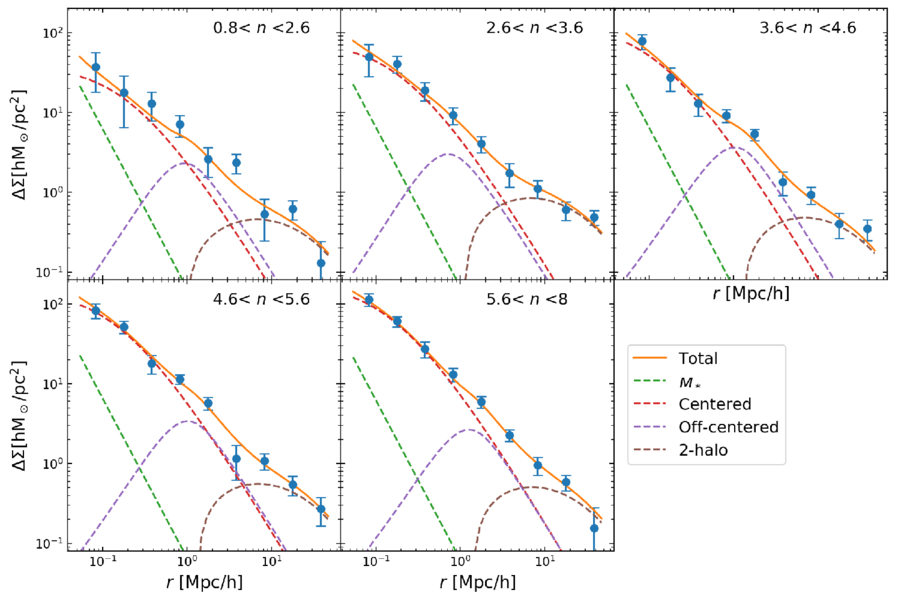
Figure 1. Measurement of the lensing ESD around central galaxies with different Sérsic indices n. Solid lines represent the best-fit curves, and dashed lines represent the ESD of different components, including stellar mass, well-centered portion, off-centered portion, and two-halo term.
Download figure:
Standard image High-resolution image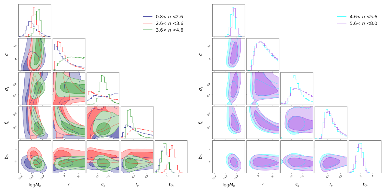
Figure 2. The 68% and 95% confidence level contour plots of five free parameters for “All” samples with different Sérsic indices.
Download figure:
Standard image High-resolution image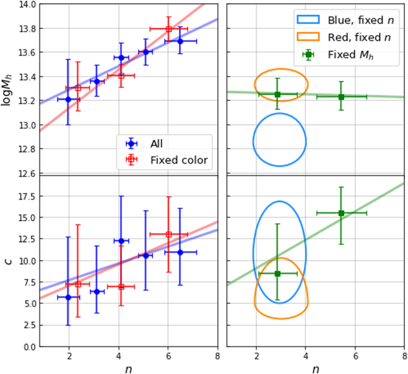
Figure 3. Best-fit halo mass  and concentration c under different conditions. Blue dots represent all samples with different Sérsic indices n, and red dots represent results for different n with fixed sample color. Light blue and orange rings represent results for blue and red galaxies, respectively, while fixed n, with ring size representing the 1σ range.
Download figure:
Standard image High-resolution imageAdditionally, we observe possible evidence that more concentrated galaxies (high n) may reside in more concentrated halos (high c), although the uncertainties are relatively large with current data. We fit the blue dots in the figure using linear relationships, yielding:


Nevertheless, due to the large uncertainties and the strong degeneracy between the concentration parameter c and the off-centering fraction fc, as shown in Figure 2, higher-quality data are required to validate our findings. Our best-fit results suggest that only about 50% of galaxies in our sample reside at the true centers of their halos, consistent with previous weak lensing studies using analyses (e.g., W. Luo et al. 2018; J. Wang et al. 2022). In contrast, some theoretical studies based on semianalytical and hydrodynamical models report lower off-centering fractions (e.g., Planck Collaboration et al. 2013; W. Wang et al. 2019). Further investigation is necessary to reconcile these differences and confirm the observational results.
Assembly bias refers to the phenomenon where the clustering of dark matter halos is influenced not only by their mass but also by their formation history and surrounding environment (R. H. Wechsler et al. 2006; N. Dalal et al. 2008). This means that halos of the same mass, but with different formation processes or environments, could exhibit different halo bias. We also set the halo bias bh as a free parameter in the hope of detecting assembly bias, and show the ratios of the measured bias bh to the theoretical value bh(Mh, z) modeled by J. L. Tinker et al. (2010) in Table 2. But for subsamples of “All,” we do not observe a clear trend of bh or assembly bias varying with n.
4.2. The Effect of Galaxy Color and Morphology
In terms of galaxy properties, higher Sérsic indices are typically associated with early-type galaxies with red colors, while lower Sérsic indices refer to late-type galaxies with blue colors (see, e.g., Figure 1 of K. Xu & Y. Jing 2022). It has long been recognized that red and blue galaxies exhibit distinct SHMR (e.g., S. More et al. 2011; Y.-j. Peng et al. 2012; W. Wang & S. D. M. White 2012; A. Rodríguez-Puebla et al. 2015; R. Mandelbaum et al. 2016; L. Posti & S. M. Fall 2021; W. Wang et al. 2021; K. Xu & Y. Jing 2022; P. Alonso et al. 2023), with red galaxies hosted by more massive dark matter halos than blue ones at fixed stellar mass. Given the strong correlation between morphology and color, it is crucial to determine which of these secondary dependencies is more fundamental. Does the halo mass dependence on n arise due to color, or is it the other way around?
Therefore, we select galaxies with rest-frame u − r colors in a narrow range of 2.3–2.7. We divide them into three subsamples according to the Sérsic index, 0.8 < n < 3, 3 < n < 5, and 5 < n < 8. To eliminate the correlation between color and n, we resample their color distributions to make them similar by randomly removing some galaxies. The left panel of Figure 4 shows their ESD measurements. The red empty squares with error bars in Figure 3 show the best-fit Mh and c versus n, and the “Fixed color” row in Table 2 presents the best-fit parameters and associated errors. We find that, after fixing the color, the dependencies of both Mh and c on n are still consistent with, and even stronger than, the results for the blue dots. The best-fit relations are


This implies that the correlation between n and halo properties is not predominantly driven by differences in the galaxy color.
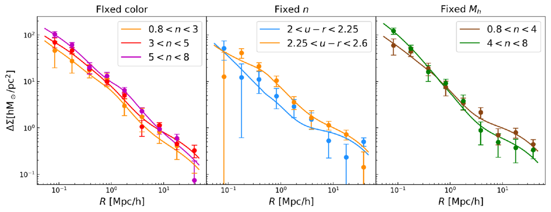
Figure 4. Dots with error bars are measured lensing ESD signals. Solid lines are the best fits. In the left, middle, and right panels, galaxies are grouped according to their Sérsic indices at fixed color, by color at fixed Sérsic index, and by Sérsic indices at fixed host halo mass obtained through abundance matching. These are indicated by different colors (see the legend).
Download figure:
Standard image High-resolution imageConversely, to explore whether the color dependence is driven by morphology, we also select galaxies with 1 < n < 6 and divide them into two color subsamples: blue galaxies with 2 < u − r < 2.25 and red galaxies with 2.25 < u − r < 2.6. For fair comparison, these two subsamples are resampled by randomly selecting galaxies to ensure a similar distribution of n, with average n of 2.98 ± 1.07 and 3.10 ± 1.09, respectively, where the errors are the standard deviations of n. The middle panel of Figure 4 shows their ESD measurements. The orange and blue rings in Figure 3 represent the results for the red and blue galaxy samples, with their sizes indicating the 1σ error range. The “Fixed n” section in Table 2 shows the best-fit results. We find that even when n is fixed, halo mass still exhibits a color bimodality, with red galaxies residing in more massive halos than blue galaxies, while their halo concentrations remain consistent. This suggests that a better secondary proxy for halo mass should involve a combination of both color and morphology. Due to data limitations, we are unable to determine the optimal combination, but this presents an intriguing topic for future research.
4.3. Halo Mass Dependence on Group Richness or Satellite Distribution
Galaxy properties and evolution are typically shaped by their surrounding environment, including local matter density and the evolutionary history of their host halos. We further investigate the properties of galaxy groups hosting the central galaxies using the group catalog from X. Yang et al. (2021), which provides details on group richness λ and member galaxies. However, galaxy/group samples from observations are generally flux-limited. As shown in the left panel of Figure 5, which plots the luminosity versus photo-z diagram of all member galaxies in groups, the member galaxies and their richness are influenced by different absolute magnitude limits at various redshifts. To mitigate the effects of redshift dependence, we define a volume-limited sample by setting a minimum luminosity threshold for the member galaxies. Consequently, the richness here is defined as the number of member galaxies in a group with  .
.
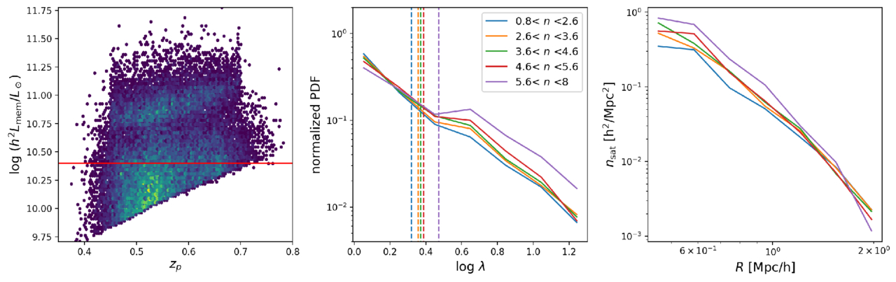
Figure 5. The left panel displays the luminosity vs. photo-z diagram of all member galaxies in clusters, with the red solid line indicating the minimum luminosity threshold used to select the member galaxies for the middle and right panels. The middle panel shows the normalized richness distribution of galaxy clusters with different galaxy Sérsic indices, where dashed lines represent the average richness of each subsample. The right panel displays the projected number density profiles of companion galaxies as a function of the projected radius.
Download figure:
Standard image High-resolution imageThe middle panel of Figure 5 shows the richness distributions of groups with different n of central galaxies in our sample. The vertical dashed lines indicate the mean richness for each sample. We find that central galaxies with larger n are more likely to be located in groups with higher richness. Also, we calculate the projected number density profiles of satellite galaxies at various projected radii, displayed in the right panel of Figure 5. It shows that the surrounding density of companion satellite galaxies increases with the n of central galaxies, consistent with the results from K. Xu & Y. Jing (2022). In fact, many previous studies have pointed out the tight correlation between the host halo mass and cluster richness or satellite abundance (e.g., E. Rozo et al. 2009; S. Andreon & M. A. Hurn 2010; W. Wang & S. D. M. White 2012; M. Simet et al. 2017; R. Murata et al. 2018, 2019; I. N. Chiu et al. 2020; A. Phriksee et al. 2020; J. L. Tinker et al. 2021; W. Wang et al. 2021; M. Chen et al. 2024), and thus our results here are related to the fact that galaxies with larger Sérsic indices are hosted by more massive dark matter halos.
4.4. Interpretations on the Correlation between Halo Concentration and Galaxy Sérsic Index
In Figure 3, we find a slight positive correlation between the Sérsic index and halo concentration. Also, the right panel of Figure 5 shows that for galaxy clusters with smaller n, the distribution of satellite galaxies is slightly more extended. While more precise measurements are needed to fully confirm this relation, it would be intriguing to explore its theoretical implications.
Numerical simulations predict the trend of lower concentrations in more massive halos (e.g., A. V. Maccio et al. 2007; A. R. Duffy et al. 2008; R. Mandelbaum et al. 2008; A. D. Ludlow et al. 2014, 2016; C. A. Correa et al. 2015; B. Diemer & A. V. Kravtsov 2015), which can be explained by that these halos form later, allowing more material and subhalos to continuously accrete from the surrounding regions, resulting in a more diffuse distribution (e.g., M. Fong & J. Han 2021; B. Diemer 2022; H. Gao et al. 2023; J. He et al. 2024). However, in our results, we find that both the host halo mass and halo concentration are positively correlated with the Sérsic index of galaxies (showing positive n–Mh and n–c relations). If the n–c relation were solely driven by the negative halo mass–concentration relation for dark matter halos, we would expect a negative n–c relation instead. Therefore, the positive correlation we observe between halo concentration and the Sérsic index is likely driven by other factors beyond the typical mass–concentration relation influenced by the environment.
J. F. Navarro et al. (1997) propose that older halos, which formed in higher cosmic densities, tend to have larger characteristic densities and concentrations. Using high-resolution N-body simulations, D. Zhao et al. (2009) find that the halo concentration is tightly correlated with the Universe age when its progenitor first reaches 4% of their current mass, i.e., t/t0.04 in their work. Therefore, we speculate that two main factors may influence the n–c relation in our results. One is introduced by the halo mass–concentration relation, that the positive n–Mh relation would introduce negative correlations between n and c. The other is that more concentrated galaxies with larger Sérsic indices form earlier at fixed stellar mass, with their host halos forming earlier as well, and dark matter halos with earlier formation times have larger concentrations. Among these two factors, the latter may play a dominant role for our galaxy samples.
To further test our hypothesis, we control halo mass in the sample by using the halo mass from the group catalog MG, which is assigned using the abundance matching technique (X. Yang et al. 2021). Considering the positive correlation between the Sérsic index n and halo mass Mh, we could adjust the selection range of MG to ensure the halo mass is the same for different galaxy samples. In particular, we divide the sample into two groups based on Sérsic index: for galaxies with 0.8 < n < 4, we select samples satisfying 1013.3 < MG < 1013.8M⊙ h−1; for galaxies with 4 < n < 8, we use samples with 1013.3 < MG < 1013.7M⊙ h−1. The right panel of Figure 4 shows the ESD measurements, Table 2 presents sample information and best-fit parameters, which are also shown by the green squares in Figure 3. We find that the halo masses from the group catalog of the two subsamples are very consistent, but halo concentrations for galaxies with larger Sérsic indices are higher, still consistent with the n–c relation shown and discussed earlier. Furthermore, compared to the n–c relation without controlling halo mass, the relation becomes steeper. This implies that by reducing the negative Mh–c relationship caused by accretion and merging, the positive correlation between n and c becomes slightly strengthened. This also supports our speculation that the host halos of galaxies with higher Sérsic indices are formed earlier, leading to higher halo concentrations, and this effect is stronger than the influence of later-time halo mergers to decrease the concentration, at least for the massive CMASS galaxies at z ∼ 0.57.
From the perspective of assembly bias, we find that the halo bias of the galaxy sample with a higher Sérsic index is lower, which is also reflected in the lower large-scale ESD shown in Figure 4. R. H. Wechsler et al. (2006) proposed that for massive halos with fixed halo mass, those that form earlier (with higher concentration) have weaker clustering, resulting in a smaller halo bias. From this standpoint, our findings further support the inference that halos hosting galaxies with higher Sérsic indices formed earlier. This also suggests that the Sérsic index could serve as a proxy for halo concentration or formation time, which could be used in the future to probe the assembly bias of galaxy clusters.
4.5. Comparison with Other Results
Figure 6 compares our main results (blue dots) with those obtained using the PAC method in the work of K. Xu & Y. Jing (2022; orange squares). To ensure a consistent basis for comparison, we convert the halo masses in our results to their definition, where Δvir = 18π2 + 82x − 39x2 and x = Ωm(z) − 1. We observe that our results systematically yield higher halo masses. This discrepancy may stem from the assumption in K. Xu & Y. Jing (2022) that massive central galaxies are perfectly situated at the halo centers, neglecting the off-centering effects in observations. By setting fc = 1 in our model, disregarding the central offsets, we show the fitting results as green hollow points in the figure. In this test, our results align well with theirs.
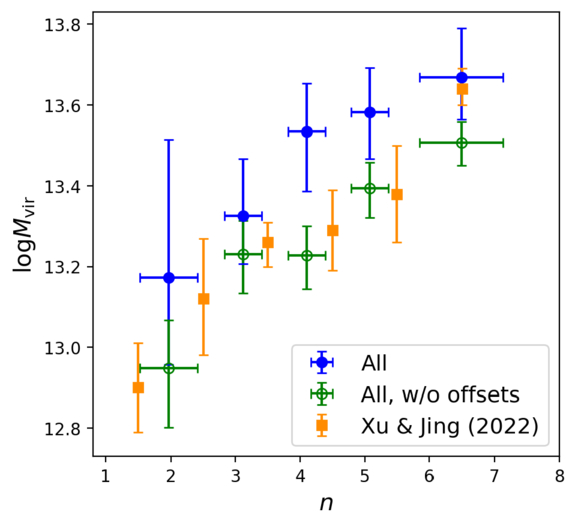
Figure 6. Relationships between n and the halo mass measured in different ways. The definition of the halo mass Mvir here is from G. L. Bryan & M. L. Norman (1998). Blue dots represent our results for all samples. Green hollow points indicate the results obtained without considering off-centering effects in the halo model. Orange squares display the results from K. Xu & Y. Jing (2022).
Download figure:
Standard image High-resolution image5. Comparison with Simulations
So far, we have probed how the host halo properties correlate with galaxy and galaxy cluster properties. However, the physical drivers behind these relationships are still under debate. W. Cui et al. (2021) quantitatively reproduce the color bimodality of the SHMR in the SIMBA simulations (R. Davé et al. 2019), showing that red galaxies reside in more massive halos at a given stellar mass. They find that this is mainly due to AGN feedback in the form of jets and X-rays, which significantly suppresses star formation earlier in red galaxies while their halos continue to grow. This could also be the reason for the n–Mh relationship. Therefore, we further investigate similar relations in this section, using two hydrodynamic simulations, TNG and SIMBA.
5.1. The Relationship between the Sérsic Index and Halo Properties
Before proceeding, we need to clarify some problems when measuring the galaxy morphology in SIMBA: the galaxies in these simulations generally exhibit very low galaxy concentrations, with n not exceeding 2. According to R. Davé et al. (2019), the size of low-mass quenched galaxies in SIMBA is a notable failure of the current model, as their half-light radii are larger than those of star-forming galaxies, which contradicts observational trends. A larger radius usually implies a lower concentration, leading to elliptical galaxies that should have higher n, but obtaining very low n values in the simulation. Nevertheless, we endeavor to incorporate the results from SIMBA in our analysis within the limited range of n it produces.
First, we use snapshots from TNG300 and SIMBA at two redshifts for the main analysis, z = 0 and z = 0.55, respectively.6 Figure 7 displays the relationships between the Sérsic index, n, and the halo mass, Mh, halo concentration, c, and richness, λ, for central galaxies in simulations. The properties of galaxies and halos are represented by scatter plots, with the linear fits represented by lines, and the 16–84th percentiles displayed as shaded areas. Note that, since there is a slight correlation between n and M*, we randomly remove galaxies at different n to decorrelate these two parameters. As a result, the slope of the relationship in the leftmost panel of Figure 7 is zero, thereby avoiding the impact of stellar mass on other correlations between n and halo properties.
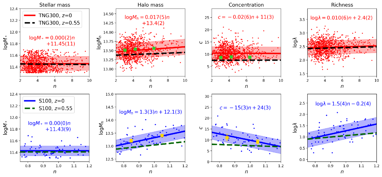
Figure 7. Correlations between the Sérsic index (n) of central galaxies and their host halo mass, halo concentration, and richness in two simulations, S100 and TNG300. Central galaxies are selected to have stellar masses in the range of  for snapshots at redshifts of 0 and 0.55. Solid lines represent linear best-fit results for samples at z = 0 (dots), with shaded areas indicating the 16th to 84th percentiles. Dashed lines represent the fitting results for samples at z = 0.55. The formula provided in each panel gives the best-fit result to galaxy systems at z = 0, in which the numbers in the parentheses represent the 1σ errors of the last digit or last two digits. The squares in the
  and c–n panels represent the best-fit results from the stacked ESD measurements in Figure 8, where the error bars are too small to be visible.
Download figure:
Standard image High-resolution imageWe also bin the galaxies into three groups in TNG300 and two groups in S100, and stacked their ESDs as in the observations. The results are presented in Figure 8 with their best-fit curves. Similar to fitting individual halos, we assume that the central galaxies in the simulations are well-centered and treat Mh, c, and bh as free parameters for fitting. The fitting results for Mh and c are shown as green and yellow squares in Figure 7. Note that the error in the stacked fitting results represents the uncertainty of the average properties of halos, which is so small that it is almost invisible in the figure. The stacked fitting results are close to the best-fit solid lines of scatter points obtained from fitting individual halos, demonstrating the robustness of the stacking lensing measurements.
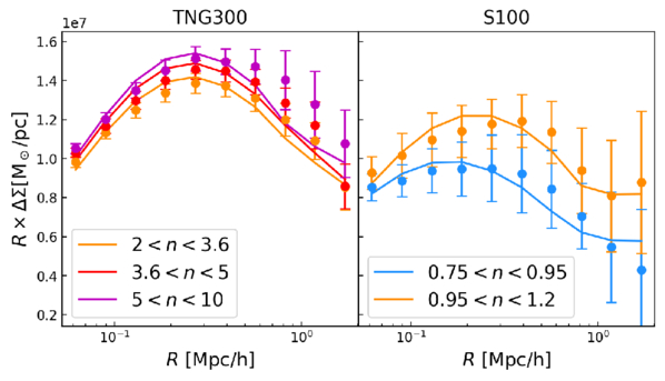
Figure 8. Dots with error bars are stacked ESDs of halos in Figure 7 within different ranges of the Sérsic index n. Solid lines are the best fits with 3 free parameters: Mh, c, and bh. The left panel shows the results from TNG300, corresponding to the upper panels of Figure 7, while the right panel is for S100, corresponding to the lower panels of Figure 7.
Download figure:
Standard image High-resolution imageRegarding the relationship between halo mass and n, we find that both TNG300 and SIMBA exhibit correlations, also shown by the rising ESD in Figure 8. However, compared to observational results, halo masses from TNG300 are higher, and their correlation with n is weaker (Equation (15)). While the S100 simulation shows a stronger correlation, considering its incorrect galaxy morphology, we only qualitatively analyze the trends. Both simulations demonstrate a positive correlation between n and halo abundance λ, which is qualitatively consistent with our results (Figure 5). Moreover, we note that the correlations between n and other galaxy and halo properties at higher redshift are weaker than those at lower redshift.
However, neither of the two simulations reproduces significant positive correlations between halo concentration and n as have been observed in the real data. A strong negative correlation even shows in SIMBA. As previously discussed, the n–c relation at fixed stellar mass is affected by: (1) the mass–concentration (Mh–c) relation of dark matter halos; and (2) the intrinsic n–c relation at fixed halo mass. To check whether the TNG simulation reveals a similar trend between n and c as what we have inferred from the data, we control both halo mass and stellar mass in a subsample from the TNG300 at z = 0. The left panel of Figure 9 shows the correlation between halo mass and stellar mass for the red points in Figure 7, color coded by n. We select galaxies within the red box in the panel and replot the correlations between n and other properties for them in the right panels of Figure 9. We find that after controlling both the stellar mass and halo mass to a narrow range, the halo concentration shows a slight positive correlation with n. This might imply that, for central galaxies with the same stellar mass and halo mass, more concentrated central galaxies are more likely to reside in more concentrated halos, which is consistent with our previous hypothesis and results. However, the correlation is still weak and may depend on the details of galaxy formation models adopted in the simulations and how realistic these models are.
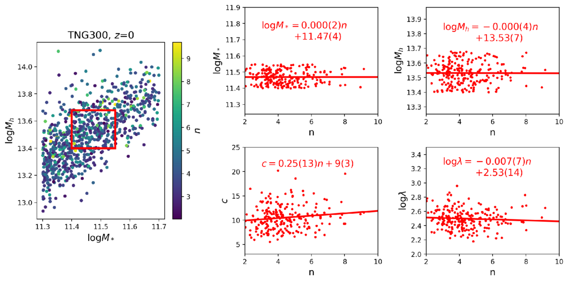
Figure 9. The left panel shows the halo mass (Mh) as a function of the stellar mass (M*) for samples in the TNG300 simulation at z = 0 (red dots in Figure 7), color coded by their Sérsic indices, n. We select the subsample within the red box to simultaneously control both M* and Mh. The right panel displays the dependencies of the Sérsic index, n, on the stellar mass, halo mass, halo concentration, and richness for this subsample.
Download figure:
Standard image High-resolution image5.2. The Effects of AGN Feedback in SIMBA
We further examine the relationship between n and the BH mass MBH in the galaxies for the two simulations at z = 0, as shown in Figure 10. We find a weak positive correlation between n and MBH in both TNG300 and S100. It might be because a larger n typically implies that a galaxy has a more dominant bulge component, and many studies reported a positive correlation between the bulge and BH mass (R. J. McLure & J. Dunlop 2002; A. Wandel 2002; N. J. McConnell & C.-P. Ma 2013; B. L. Davis et al. 2019). We also display the relationship between MBH and Mh, revealing strong positive correlations. We can derive the relationship between  and n by combining the best-fit equations in the
  and
and  panels, and we find that the results are consistent with those obtained from the direct fitting shown in Figure 7. This implies that the correlation between the Sérsic index and halo mass might be related to the different BH activities.
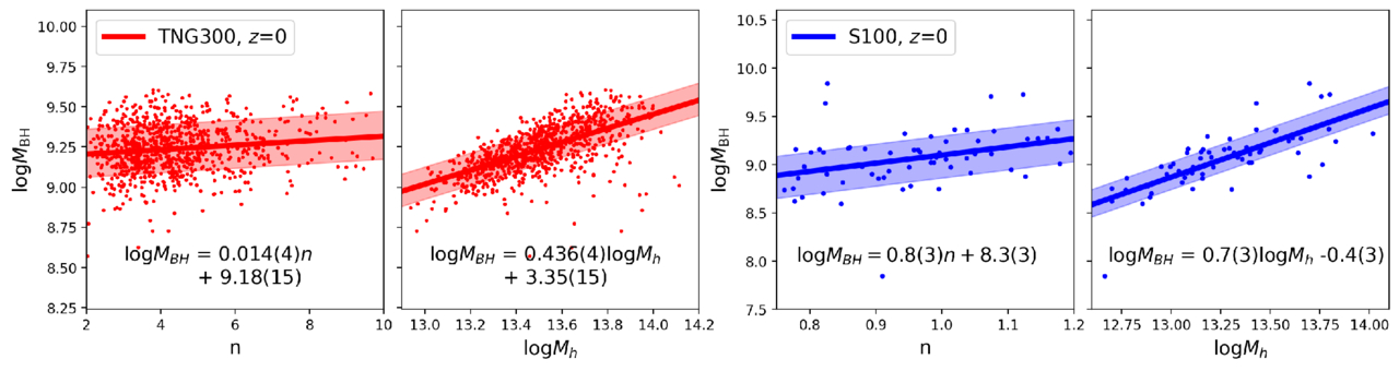
Figure 10. Relationship among n, black hole mass MBH, and halo mass Mh for galaxies from S100 and TNG300 at z = 0 (corresponding to the red and blue dots in Figure 7). The solid lines represent linear best-fit results, and shaded areas represent the 16th to 84th percentiles. The formulae in the panels are equations of the solid lines.
Download figure:
Standard image High-resolution imageAccording to N. Thomas et al. (2019), the Eddington ratio, fEdd, of BHs is inversely correlated with their mass. When fEdd < 0.2, it would trigger jet-mode AGN feedback and subsequent X-ray AGN feedback. Therefore, to validate the n–Mh relationship in SIMBA influenced by BH mass, we use simulations from the SIMBA series with different modes of AGN feedback, including simulations that incorporate all physical processes (“S50”), that exclude X-ray feedback (“S50, no-X”), and that exclude both X-ray feedback and jet-mode AGN feedback (“S50, no-jet”). Figure 11 shows the correlations between n of central galaxies and other halo properties for three simulations, where the shaded regions represent the 16–84th percentiles. We observe distinctly different trends of n with other properties in the three simulations. As shown in the leftmost panel, the average stellar mass of galaxies without X-ray and jet-mode AGN feedback (orange) is higher than those with jet-mode AGN feedback (red and blue). This indicates that jet-mode feedback primarily reduces the star formation rate in galaxies, as stated in R. Davé et al. (2019). Furthermore, as AGN feedback modes are progressively turned off, the slope between halo mass and n gradually decreases. Especially in the “S50, no-jet” simulation, the correlation between n and Mh almost disappears, and the correlations with c and λ are also significantly weakened. These results indicate that the relationship between n and halo properties might be influenced by the strength of AGN feedback, especially the jet mode, which can rapidly and effectively expel gas from galaxies, leading to the cessation of star formation.
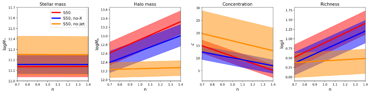
Figure 11. Similar to Figure 7, but the results are from three different simulations. “S50” represents the SIMBA simulation with a box length of 50 Mpc/h. “no-X” indicates a simulation without X-ray feedback, and “no-jet” represents a simulation without X-ray and jet-mode AGN feedback.
Download figure:
Standard image High-resolution image6. Summary and Conclusion
We delve into the relationship between the morphology of central galaxies indicated by the Sérsic index, n, and the properties of their host dark matter halos and galaxy groups/clusters, including the halo mass, halo concentration, and group richness. Our study in this paper extends the work of K. Xu & Y. Jing (2022), in which the morphology, color, and size dependencies of the SHMR for massive central galaxies have been investigated using the PAC method. We use the central galaxy sample from their work, with a mass range of  and a redshift range of 0.45–0.7, selected from BOSS CMASS observations. We employ galaxy–galaxy lensing to measure the ESD around these galaxies, using the Fourier_Quad shear catalog from the third public data release of HSC. In our modeling approach, the halo mass Mh and concentration c from the NFW profile were considered as free parameters, while also incorporating off-centering effects and two-halo terms. We find the following:
- 1.From lensing measurements, we discover a strong positive correlation between the halo mass and the Sérsic index n of central galaxies with fixed stellar mass, demonstrating that more concentrated central galaxies reside in more massive halos.
- 2.To investigate whether the galaxy Sérsic index, n, or galaxy color is a more fundamental secondary property in determining halo mass, we separately control n and color for galaxies to be in a narrow range. The dependence of the halo mass on both n and galaxy color still exists, which might indicate that some combinations of color and n can be a better secondary proxy.
- 3.We find a slight positive correlation between n and halo concentration c with postive n–Mh relations. In contrast, the simulation results show that more massive halos are less concentrated due to their more frequent mergers in the late Universe. After controlling for both the stellar mass and halo mass, we observe a slight strengthening of the n–c dependence. This suggests that the n of galaxies may serve as an indicator for the secondary Mh–c relation, which contributes to the scatter of the general Mh–c relation in simulations. We therefore infer that, at fixed stellar mass, more concentrated galaxies and their host halos form earlier and have higher concentrations.
- 4.Using the group catalog from X. Yang et al. (2021), we find that more concentrated central galaxies are located in richer galaxy clusters and have a higher average satellite galaxy number density around them.
- 5.TNG300 and SIMBA simulations qualitatively reproduce the positive correlation between n and the halo mass as well as richness, but the correlation in TNG300 is very weak. Additionally, neither simulation shows positive n–c relationships. By further controlling the halo mass in the TNG300 sample, we find a weak positive n–c correlation.
- 6.In TNG300 and SIMBA, there are slight positive correlations between n and the BH mass, and strong positive correlations between the BH mass and halo mass. As we progressively turn off X-ray feedback and jet-mode AGN feedback in SIMBA simulations, the correlation between n and the halo mass gradually disappears. This suggests that AGN feedback might play a role in the halo mass dependence on secondary galaxy properties mentioned above.
Our detection of the halo mass dependence on secondary galaxy properties brings better insights into the physics of galaxy assembly bias, which is an important problem in the current galaxy–halo connection field. With next-generation surveys and better measurements, the connection between galaxies and halos should be better constrained.
Acknowledgments
This work is supported by the National Key Basic Research and Development Program of China (2023YFA1607800, 2023YFA1607802), the NSFC grants (11621303, 11890691, 12073017), and the science research grants from China Manned Space Project (No. CMS-CSST-2021-A01). Z.L. is supported by the funding from the China Scholarship Council. K.X. is supported by the funding from the Center for Particle Cosmology at U Penn. W.W. is supported by NSFC (12273021) and the National Key R&D Program of China (2023YFA1605600, 2023YFA1605601). The computations in this paper were run on the π 2.0 cluster supported by the Center of High Performance Computing at Shanghai Jiaotong University and the Gravity supercomputer of the Astronomy Department, Shanghai Jiaotong University.
The Hyper Suprime-Cam (HSC) collaboration includes the astronomical communities of Japan and Taiwan, and Princeton University. The HSC instrumentation and software were developed by the National Astronomical Observatory of Japan (NAOJ), the Kavli Institute for the Physics and Mathematics of the Universe (Kavli IPMU), the University of Tokyo, the High Energy Accelerator Research Organization (KEK), the Academia Sinica Institute for Astronomy and Astrophysics in Taiwan (ASIAA), and Princeton University. Funding was contributed by the FIRST program from the Japanese Cabinet Office, the Ministry of Education, Culture, Sports, Science and Technology (MEXT), the Japan Society for the Promotion of Science (JSPS), the Japan Science and Technology Agency (JST), the Toray Science Foundation, NAOJ, Kavli IPMU, KEK, ASIAA, and Princeton University.
This publication has made use of data products from the Sloan Digital Sky Survey (SDSS). Funding for SDSS and SDSS-II has been provided by the Alfred P. Sloan Foundation, the Participating Institutions, the National Science Foundation, the U.S. Department of Energy, the National Aeronautics and Space Administration, the Japanese Monbukagakusho, the Max Planck Society, and the Higher Education Funding Council for England.
Appendix A: Field Distortion Test
Here, we measure the multiplicative biases introduced in shear measurements and correct them in our analysis. Such biases arise from systematic errors or the intrinsic noisiness of the shear estimators, and they are typically quantified linearly

where mbias is multiplicative bias and cbias is addictive bias, gtrue refers to the real shear, and gobs represents the measured shear.
In an ideal scenario, astronomical observation equipment should provide distortion-free images. However, the images are always distorted due to imperfections in the optical system or imaging equipment, known as field distortion (FD). This distortion affects the shapes and the positions of galaxies and stars, introducing an equivalent shear, with two components denoted as gf1 and gf2. It is typically related to the object’s position on the focal plane rather than its position in the sky. J. Zhang et al. (2019) proposed using FD to detect cbias and mbias in shear measurements, which is a calibration method based on the properties of the data themselves. The two components of the FD signals of each galaxy, gf1 and gf2, are provided in the FQ shear catalog. By stacking the galaxy shear estimators at fixed FD values, the cosmic shear signal will vanish since these galaxies are from different positions on the sky, allowing us to recover the FD value. By comparing the measured FD signals with the true FD signals from the catalog and using Equation (A1), the shear bias in the measurements can be determined.
We perform an FD test on all background galaxies in the ESD measurements, and we weight each background galaxy by Σc (Equation (3)) to better match the ESD scenario. Since we use background galaxies with ∣gfi∣ < 0.02(i = 1, 2), we divide gfi evenly into 10 bins from −0.02 to 0.02, and stack the galaxy shear estimators within each bin to calculate the observed shear value  . Figure 12 displays the measured signals for the two shear components, where gf is the true FD value, and the vertical axis represents the difference between the observed distortion value
  and the true value. If there is no shear measurement bias, the results in the plot should all align with 0, i.e.,
  . The figure also shows the shear bias results obtained from fitting, revealing that the g1 component is underestimated by about 3%. Consequently, we correct the shear estimators Gi (i = 1, 2) in the catalog as Gi/(1 + mi) before performing galaxy–galaxy measurements in Equation (4). Additionally, cbias is largely mitigated by rotating background galaxies toward the lenses during galaxy–galaxy lensing calculations, with further reduction through the subtraction of random point signals.
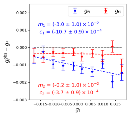
Figure 12. Field distortion test. gf represents the field distortion values from the shear catalog, while the vertical axis represents the difference between measured values  and true values. Blue and red correspond to the two components of the shear. mi and ci represent the multiplicative and additive biases obtained from linear fitting, respectively.
Download figure:
Standard image High-resolution imageAppendix B: The ESD Model of a Galaxy
In this study, we assume that galaxies can be treated as point sources for measuring the ESD. The purpose of this section is to show that, within the radial range measured in this work, using point sources does not significantly affect the ESD results. Typically, assuming a constant mass-to-light ratio within galaxies, their light distribution can be considered the same as their mass distribution. A more accurate ESD model would involve using the Sérsic profile from Equation (1) in Equation (2) to calculate the ESD. However, when measuring the ESD of halos, galaxies are often treated as very small compared to the halos and are approximated as point sources, meaning their density profile is a Dirac delta function δ(r). Since the minimum radius for our ESD measurement is set at 0.05 Mpc h−1, which is comparable to the size of galaxies. Therefore, we need to verify whether the point-source model is valid at this scale. In the TNG300 simulation described in Section 5, the average half-light radius Re of the galaxies shown in Figure 7 is about 20 kpc h−1. Using this, we create a simple Sérsic profile and set the galaxy mass to 1011.5M⊙. Figure 13 shows the ESD results for two models. It is clear that within the white region (the radial range in our measurement), the ESD results from both models are almost identical, but the point-source model would overestimate at smaller scales (gray region). Thus, within the current radial range, using the point-source model for simplified calculations does not affect the reliability of the conclusions in this paper.
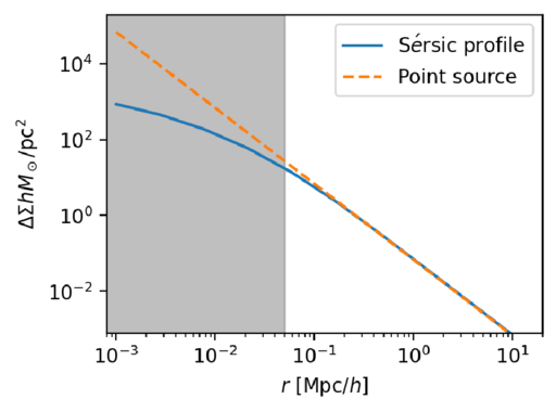
Figure 13. ESD of a galaxy using a Sérsic profile and a point-source model. The white region represents the radius range in our measurements.
Download figure:
Standard image High-resolution imageFootnotes
- 5
We made our results public on https://github.com/load666/arXiv-2411-07525/.
- 6
The latter is actually z = 0.556839 for SIMBA, but denoted as 0.55.