Based on modern cosmology, the large scale of the Universe grew from the small perturbation seeded by the inflation during the Big Bang (P. J. E. Peebles 1980; J. F. Navarro et al. 1996; S. Cole et al. 2000; S. Dodelson 2003; S. Stierwalt et al. 2017). Due to gravitational instability, dark matter started to cluster and formed into isolated structures known as halos, which are the homes of galaxies and galaxy clusters. Dwarf galaxies (DGs) reside in small dark matter halos and can be treated as the building blocks of larger galaxies. Therefore, studying the evolution of DGs is crucial for understanding the formation and evolution of more massive galaxies, such as the Milky Way.

The circumgalactic medium (CGM) and the intergalactic medium (IGM) surrounding the DG can affect its evolution significantly. Both models (G. S. Stinson et al. 2012; A. B. Ford et al. 2013; S. Shen et al. 2013; J. Suresh et al. 2017) and observations (C. Brüns et al. 2000; M. Walker 2013; L. Anderson et al. 2014) suggest that the CGM contains a highly dynamic multiphase structure of gas density, temperature, and metallicity (J. Tumlinson et al. 2013, 2017; K. Tchernyshyov et al. 2022). However, the IGM contains hot ionized gas residing in the filament and void of large-scale structures. The IGM comprises most of the baryon and dark matter of the Universe and constitutes the bedrock of the formation of cosmic structures (J. P. Macquart et al. 2020). Some gas from the CGM and IGM can cool through radiative processes and eventually accrete onto galaxies, fueling star formation (SF). Meanwhile, feedback from massive stars, their supernovae (SNe), and the accreting supermassive black hole (SMBH) returns energy and gas from galaxies to the CGM and IGM. This in-and-out feedback loop results in a baryonic ecosystem that can sustain and regulate galactic SF (G. M. Voit 2019; J. J. Davies et al. 2020; B. D. Oppenheimer et al. 2020; B. A. Terrazas et al. 2020; E. Zinger et al. 2020). Therefore, the IGM and CGM can significantly affect the evolution of a galaxy and prevent gas depletion for SF (R. B. Larson 1972; R. B. Larson et al. 1980; B. M. Tinsley 1980; J. X. Prochaska & A. M. Wolfe 2009; C.-A. Faucher-Giguère et al. 2011; C. Péroux & J. C. Howk 2020).

The accretion of the CGM and IGM onto a galaxy depends on its halo mass and environment, which are influenced by the galaxy’s location and redshift. A. Dekel & J. Woo (2003) and D. Kereš et al. (2005) have proposed two distinct accretion modes: cold and hot. The mode of accretion depends on the competition between the cooling time (t_c) and the freefall time (t_ff). If t_c < t_ff, the accreting gas can cool before being accreted, resulting in cold accretion. For hot accretion, t_c > t_ff, the gas remains hot during accretion. Cold accretion is more efficient, because the accreting flow is unshocked with a lower temperature (T ∼ 10⁴ K). Since the temperature of the accreting gas is determined by the gravitational potential of a halo, generally speaking, cold accretion occurs in halos of virial mass M_vir < 3 × 10¹¹ M_⊙ (A. Dekel & Y. Birnboim 2006; A. Cattaneo et al. 2020), which allows the IGM gas to flow efficiently into the galaxy and form stars. Therefore, cold accretion is crucial in shaping these DGs of M_vir ≤ × 10¹¹ M_⊙.

Previous studies of the coevolution between DGs and their CGM used idealized disk galaxy models (e.g., V. Springel et al. 2005; V. Perret 2016). J. Zhu et al. (2024) examined the effect of ram pressure stripping on an idealized DG through a wind tunnel setup. Meanwhile, other related models used cosmological simulations to obtain more realistic initial conditions for DGs and their CGM. For example, F. van de Voort et al. (2012) modeled the Hi absorbers to support the evidence of cold accretion, and M. P. Rey et al. (2020) studied the evolution of ultrafaint field DGs by considering dark-matter-only cosmological simulations. W. Zhu et al. (2022) studied the accretion of the IGM from cosmic filaments and obtained the galaxy accretion rates as a function of redshift and halo mass. E. Tollet et al. (2022) derived the entropy criteria that distinguish accretion in the cold and hot modes based on NIHAO simulations (L. Wang et al. 2015). Furthermore, the FIRE team (P. F. Hopkins et al. 2014, 2018b, 2023) performed a serial study of galaxy evolution, tracking the baryon evolution of the galaxy (D. Anglés-Alcázar et al. 2017) and the CGM based on cosmological zoom-in simulations (Z. Hafen et al. 2019, 2020).

Several studies have revealed the influence of the CGM/IGM inflow and outflow on the evolution of DGs. D. Brisbin & M. Harwit (2012) show that most low-mass (M_vir ∼ 10¹⁰M_⊙) star-forming galaxies are fed by low-metallicity (Z ∼ 0.1 Z_⊙) gas infall, and Z. Hafen et al. (2019) demonstrate that the IGM dominates CGM accretion, rather than being wind-fed from central or satellite galaxies. C. R. Christensen et al. (2018) demonstrate that DGs can eject more metal into the CGM due to their shallow gravitational potential. Furthermore, about 50% of the outflowing gas from DGs falls back onto the host DGs (C. R. Christensen et al. 2016). On the other hand, the gas outflow from the CGM leaves the host halo and becomes diffuse the IGM (Z. Hafen et al. 2020). However, these previous studies did not consider the redshift evolution of DGs and their CGM from z = 2 to z = 0, which will be soon examined by James Webb Space Telescope (JWST) observations.

Although these studies provide significant insights into the evolution of DGs and their CGM, some obstacles remain. The isolated galaxy model is relatively computationally cheaper and thus can reach a higher resolution for resolving the physical processes in the interstellar medium (ISM). However, the assumption of a symmetric or isotropic CGM could be oversimplified and thus lead to less realistic results. However, cosmological simulations can generate galaxies directly from the formation of large-scale structures. Still, their low spatial resolution limits the possibility of accurately resolving the structure of the multiphase CGM, SF, and the associated stellar feedback model, which have been proven to be important in modeling galaxy evolution (J.-h. Kim et al. 2016; R. J. Wright et al. 2024). Cosmological zoom-in simulations like FIRE are feasible approaches for balancing between the simulation domain and resolution. However, these zoom-in simulations still neglect the cosmic environmental evolution of galaxies, which is critical for the formation and dynamics of the IGM and CGM.

Therefore, we perform new 3D high-resolution hydrodynamical simulations of DGs using the GIZMO code (P. F. Hopkins 2015; P. F. Hopkins et al. 2018b). Unlike previous models, we adopt the results from the state-of-the-art cosmology simulation IllustrisTNG (D. Nelson et al. 2019b) as the initial conditions for our simulations. Our simulations consider the physical processes required for properly modeling the galaxy evolution, such as gas cooling and chemistry, SF and stellar feedback, and SMBH feedback. In this work, we focus on the coevolution of DGs and their surrounding CGM and IGM at redshifts (z) of 0, 1, and 2. The goal is to better understand the evolution of DGs along with their environments across cosmic time.

We introduce the methodology of our simulations in Section 2, then present our results in Section 3. In Section 4, we discuss our results and their astrophysical implications. Finally, we conclude with our findings in Section 5.

2.1. `GIZMO` Code

We use the modified version of the hydrodynamical simulation code GIZMO, a descendant of a widely used smoothed-particle hydrodynamics (SPH) code, GADGET-2 (V. Springel 2005). GIZMO features quasi-Lagrangian numerical schemes with moving-mesh-like calculations for hydrodynamics, including meshless finite volume and meshless finite mass (MFM). The physical quantities of a gas cell are computed by the cubic spline kernel (J. J. Monaghan 1992) and evolved by solving the flux on the boundaries from the Voronoi tessellation of gas particles. These schemes combine the advantages of SPH codes, such as the conservation of angular momentum, with the accuracy of the flux calculation offered by mesh codes. Furthermore, GIZMO also includes comprehensive modules required to model the key physical processes in galaxy evolution. We describe our simulation setup and associated physics modules in the following sections.

2.1.1. Hydrodynamics

We adopt the MFM method to solve homogeneous Euler equations in the simulations. This method ensures mass conservation in each gas cell, by eliminating the mass flux between gas cells while evolving the fluid. Based on P. F. Hopkins et al. (2018b), the advantages of MFM are as follows. First, MFM couples well with the gravity solver, thus reducing the error from the self-gravity calculation of gas particles. Second, MFM is the best algorithm for precisely tracking the gas flow, due to the conservation of mass in each gas cell. Third, MFM can also reduce the numerical errors of the particle-splitting method in our simulations (see Section 2.2.2).

In addition, we also include a subgrid model of small-scale turbulence between gas particles. We adopt an eddy mixing model from J. Smagorinsky (1963) in our simulations, following M. J. Colbrook et al. (2017), P. F. Hopkins et al. (2018b), and D. Rennehan et al. (2018). This model evaluates diffusion by calculating the gradient and shear tensor. This subgrid model can drive the mixing of metallicity, velocity, and energy at the particle scale, making the simulation more physical.

2.1.2. Gas Cooling

Our gas cooling includes the combined effect of H and He cooling, collisional processes, free–free emission, molecular hydrogen, dust collisional effects, fine-structure lines, cosmic rays, and Compton effects (P. F. Hopkins 2015; P. F. Hopkins et al. 2018b). Due to the chemical enrichment from SNe, metal-line cooling is also considered, by assuming the solar abundance pattern for the enriched gas.

The molecular and fine-structure cooling is included to allow gas cooling to a temperature of ∼10–10⁴ K, to better model the galactic ISM and SF (P. F. Hopkins et al. 2018b, 2023). Instead of solving the chemical evolution, we use a fitting function from M. R. Krumholz & N. Y. Gnedin (2011) to calculate the molecular gas fraction based on the gas density and metallicity. The result of the molecular fraction is also applied in the SF routine (Section 2.1.3). Additionally, the standard UV background is incorporated into the simulations using a UV background (UVB) table, TREECOOL. The latest version of TREECOOL (C.-A. Faucher-Giguère 2020) includes the redshift correction of UVB and the effects of active galactic nucleus (AGN) feedback (J. Oñorbe et al. 2017; X. Shen et al. 2020).

2.1.3. SF and Stellar Feedback

We adopt the direct sink formation of gas cells and the stellar feedback on the surrounding cells as an IMF-averaged star cluster. With a decent gas resolution, ∼600 M_⊙ per cell, we can resolve the relevant physical scale of giant molecular clouds and apply the star cluster formation using the IMF sampling (Y. Revaz et al. 2016).

The SF routine converts a gas particle into a star particle if the following criteria are met. First, the density of the gas cell must exceed the critical density n_crit = 1000 cm⁻³, optimized for our resolution to prevent unphysical SF in low-density regions. Second, the star-forming gas cell must be surrounded by a convergent flow (∇ · v < 0 with the gas velocity, v) and remain self-gravitating (P. F. Hopkins et al. 2013). The self-gravitating (gravitationally bound) criterion ensures that a gas cell’s kinematic and thermal energy is lower than the local gravitational potential. Eventually, for any gas particle that meets these conditions, the star formation efficiency (SFE) is scaled by the molecular fraction of gas satisfying self-shielding to undergo SF (P. F. Hopkins et al. 2018b).

After a star particle forms, its stellar feedback influences the surrounding gas. We used a stellar feedback model based on the AGORA project (J.-h. Kim et al. 2016), which accounts for the time- and IMF-averaged stellar feedback from core-collapse SNe in a star cluster over 30 Myr, as most massive stars have lifetimes shorter than 30 Myr. A constant SN event rate is set, to determine the number of SNe exploding for a star particle, N_sn, at a given time step. Then, the total energy of N_sn × 10⁵¹ erg will be dumped onto the gas around the star particle in the form of kinetic energy, to prevent overcooling. The algorithm developed in P. F. Hopkins et al. (2018a) adds momentum statistically and isotropically, with a kernel-weighted evaluation, to ensure the conservation of energy and angular momentum. The momentum and energy distributed to the nearby gas are calculated on the effective faces of the Voronoi cell, constructed between the star particle and the interacting gas cells. This method can explicitly resolve the structure of the Sedov blast wave, which has been validated in previous studies (P. F. Hopkins et al. 2014; T. Kimm & R. Cen 2014; D. Martizzi et al. 2015).

2.1.4. SMBH Growth and Feedback

Since the spatial resolution of our simulations cannot resolve the accretion disk of the SMBH at the center of the DG, we use a simplified and spherically symmetric accretion model, Bondi–Hoyle accretion (H. Bondi 1952), for the SMBH accretion. The model accretes gas stochastically onto the SMBH, with the accretion rate limited by the Eddington rate (V. Springel & L. Hernquist 2003; T. Di Matteo et al. 2005), based on a radiative efficiency of _r ≈ 0.1, according to observations.

After the accretion of gas, the kinetic feedback from the disk wind is deposited onto the surrounding gas in the form of momentum (P. F. Hopkins et al. 2016). The disk wind of the SMBH follows the energy of $0.5{\dot{M}}_{{\rm{w}}}{V}_{\,\rm{w}\,}^{2}$ , with a wind velocity of V_w ∼ 10% of the speed of light and mass loading of ${\dot{M}}_{{\rm{w}}}=0.5\,{\dot{M}}_{{\rm{BH}}}$ , where ${\dot{M}}_{{\rm{BH}}}$ is the mass accretion of the SMBH. To compensate for the dynamical effect on the SMBH, we also employ a dynamical friction model for the SMBH particle, which applies the gravity-dragging force from the medium of gas and dark matter to stabilize the motion of the SMBH at the galactic center (M. Tremmel et al. 2015; C.-H. Lin et al. 2023).

2.2. Simulation Setup

2.2.1. Initial Conditions from the `IllustrisTNG` Project

To obtain realistic environments for the DG and its surroundings, we initialize our simulations with data from the state-of-the-art cosmological simulation the IllustrisTNG project. We retrieve a small volume from TNG50-1 (D. Nelson et al. 2019a; A. Pillepich et al. 2019), the highest-resolution run, and import the data into our simulations. The volume selection in TNG50-1 obeys the following criteria. First, for a given z, we select two halos of DGs with virial mass M_vir ∼ 5 × 10¹⁰ M_⊙. These two halos are located in distinct environments within the cosmic web—either at the nexus of filaments or in isolation, since we cover the halos at z = 0, 1, and 2 in the TNG50-1 simulation and we extract six halos for our simulations. Second, we limit our selection to star-forming and gas-rich halos. Additionally, each of the selected DG halos is required to contain an SMBH at its center. Third, the host DG halo should comprise >85% of the total halo mass, to exclude major mergers. Merger histories from subhalo catalogs are carefully examined, to ensure that no major mergers occurred during the evolution of our target galaxies. To evaluate the environmental and redshift effects of our selected DGs, we show the correlation of the stellar half-mass (M_⋆), the gas mass within the half-stellar-mass radius (M_gas), and the star formation rate (SFR) for our models, along with all TNG DGs at a given redshift, in Figure 1. For the z = 0, 1 DGs, the values of M_gas, M_⋆, and SFR of our models are close to the median values. For the z = 2 DGs, our models deviate more from the median values but are still within 1σ. This also implies that DGs of the same stellar mass at high z can have a larger scatter in M_gas and SFR, based on our selection criteria. If the gas-to-stellar mass ratio (M_gas/M_⋆) of a galaxy is directly correlated with its environment, then for each redshift, our two models, a and b, are separated by the median value of M_gas/M_⋆, representing galaxies in relative gas-rich and gas-poor environments, respectively.

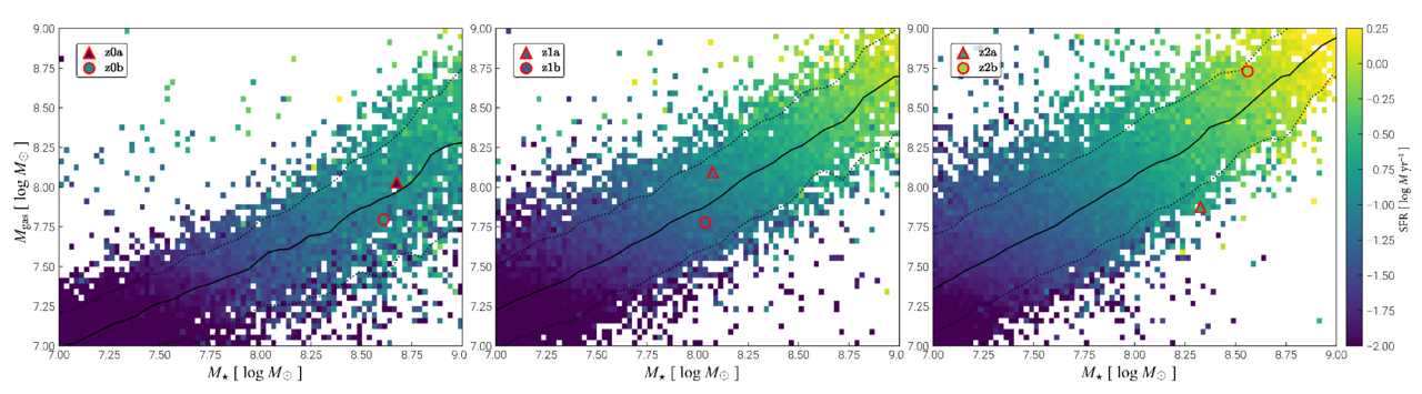
Figure 1. Refer to the following caption and surrounding text. — **Figure 1.** The correlation of M_⋆, M_gas, and SFR for DGs with M_⋆ = 10⁷–10⁹M_⊙ in TNG50-1. The panels from left to right show the DGs at z = 0, 1, and 2, respectively. Our models are annotated with circles and triangles, with the color-coded SFR given in the plots. Most of our models lie within one standard deviation (dotted lines) from the solid lines, representing the median values of M_gas for a given M_⋆. Two DGs at z = 2 are slightly away from the solid line but remain close to 1σ.
Download figure:
Standard image High-resolution image

After deciding on the targeted halos in IllustrisTNG, we retrieve a spherical volume centered on the selected halo and import it into GIZMO as the initial conditions. The radius of the sphere is 440 ckpc, corresponding to at least ∼3 R_vir. This radius is larger than the standard box size for cosmological zoom-in simulations suggested by J. Onorbe et al. (2013). Finally, we evolve our simulation for 1.5 Gyr, which is more than 10 dynamical times, to guarantee the dynamical equilibrium in the systems. We summarize our initial conditions in Table 1.

Table 1. Summary of Initial Conditions

Model	z	M_vir	R_vir^a	M_⋆	R_⋆,1/2	M_BH	Characteristics of the DG and its environment—the shape of the surrounding CGM/IGM.
		(10¹⁰ M_⊙)	(kpc)	(10⁸ M_⊙)	(kpc)	(10⁶ M_⊙)
z0a	0	2.84	64.34	5.22	3.26	3.29	This galaxy has spiral arms, and it is located in relative isolation, with a hot CGM and IGM.
z0b	0	5.09	78.14	4.14	0.89	5.32	The structure of this galaxy looks irregular, and it is surrounded by filaments of diffuse gas.

z1a	1	3.97	49.02	1.35	1.62	1.74	This galaxy looks irregular, and it moves away from filaments of diffuse gas.
z1b	1	4.55	51.30	2.54	1.18	1.58	The structure of this galaxy looks irregular, and it is close to a nearby massive galaxy located ∼200 kpc away.

z2a	2	6.30^b	40.29	3.32	1.61	1.88	The structure of this galaxy appears irregular, and it is surrounded by gas-rich filaments undergoing a minor merger with a smaller halo.
z2b	2	9.63	46.42	3.66	1.81	1.81	The structure of this galaxy appears irregular, and it is located at the nexus of several filaments.

Notes. Summary of all the halo properties, including the model name, redshift (z), virial mass (M_vir), virial radius (R_vir), stellar half-mass (M_⋆), stellar half-mass radius (R_⋆,1/2), and mass of the central SMBH (M_BH).

^aThe virial radius is defined by R₂₀₀, where the matter density reaches about 200 times the critical density of the matter in the Universe.^bFor a DG at z = 2, its halo is not fully virialized. Therefore, the virial mass calculated directly by the enclosed mass of R_vir would overestimate the actual mass. The gravitationally bounded masses for z2a and z2b are 5.13 × 10¹⁰ M_⊙ and 9.06 × 10¹⁰ M_⊙, respectively.

Download table as: ASCII Typeset image

2.2.2. Resolution

To further increase the mass resolution of the initial conditions from TNG50-1, we apply the super-Lagrangian refinement introduced in P. F. Hopkins (2015)—an algorithm for the splitting and merging of particles during the simulation, which shares a similar idea as the adaptive mesh refinement in mesh codes. A similar method is also used in the project GIBLE (R. Ramesh & D. Nelson 2024; R. Ramesh et al. 2024) to study the evolution of Milky Way–like galaxies with the AREPO code (V. Springel 2010; R. Weinberger et al. 2020), based on the initial conditions from TNG50-2. This method can increase the resolution of both dark matter and gas particles, and it works accurately with the MFM method. To ensure better spatial and mass resolution for resolving the ISM physics within a galaxy, we further implement a static and radial-dependent hierarchy refinement in our simulations. The particles within 50 ckpc have the highest resolution, and then the resolution decreases by a factor of 2 for every 50 ckpc, starting from the center of the halo defined by the SMBH.

In our simulations, we set the total baryon and dark matter particle numbers to be similar. In the central region, the optimal mass resolution reaches 600 M_⊙ for baryon particles and 10⁴ M_⊙ for dark matter particles. The baryon mass resolution in our study is carefully selected, to resolve the galactic ISM and SF. Based on the smoothing length of a particle, the highest spatial resolution is ∼4 pc for gas and ∼140 pc for dark matter. For the star-forming region, the spatial resolution of the gas is ∼5 pc on average, which ensures the convergence of the SF.

3.1. Physical Properties of DGs and Their CGM

Before we present the physical properties of the DGs and their CGM, we first define the regions of the galaxy, CGM, and IGM, based on their locations relative to the halo center, as shown in Figure 2. During the simulation, the inflow and outflow occurring in the galaxy can change the original distribution of the gas in the galaxy, CGM, and IGM. Figure 3 shows a density snapshot at the end of our simulations. Our DGs show irregular structures, because of their evolution via accretion flows from the CGM. The redshift of a DG has a strong influence on its evolution. Based on the gas density distribution, the sizes of the gaseous disks increase from z = 2 to z = 0. So the structure of the galaxy is more compact at z = 1 and z = 2, while the galaxy at z = 0 is relatively sparse and exhibits spiral arm-like structures, particularly for the DG of z0a, which is initially located in a more isolated environment, with little surrounding gas. The CGMs of z2a and z2b are filled with dense gas filaments, driving strong gas accretion onto the galaxies and shaping their irregular structures.

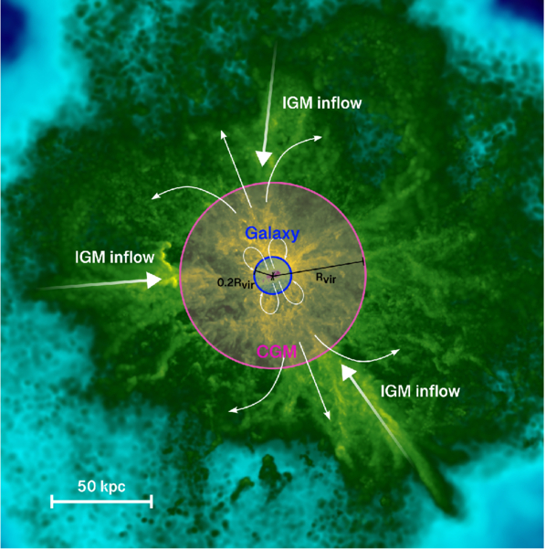
Figure 2. Refer to the following caption and surrounding text. — **Figure 2.** A schematic figure illustrates the regions of the galaxy, the CGM, and the IGM. The innermost region of 0–0.2 R_vir (blue), the intermediate ring of 0.2–1 R_vir (pink), and the outer region of >R_vir correspond to the galaxy, the CGM, and the IGM, respectively. The baryon cycle of the galaxy is demonstrated by the white arrows, indicating the inflow from the IGM, the outflow from the halo, and the recycling of gas inside the CGM.
Download figure:
Standard image High-resolution image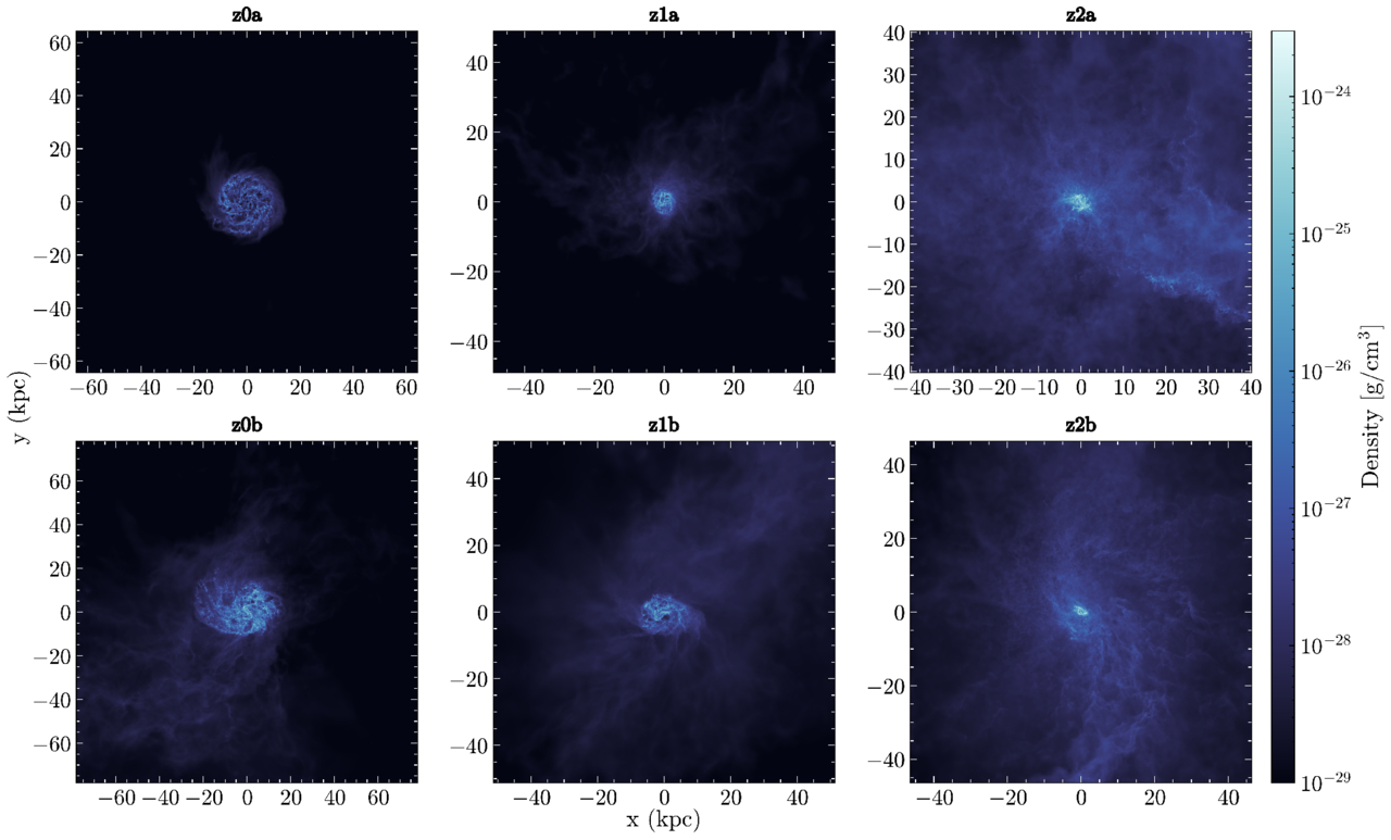

Figure 3. Refer to the following caption and surrounding text. — **Figure 3.** The gas density inside R_vir for all models at the end of the simulations. All galaxies show some diffuse structures around the major disk. The z2a and z2b models show the most prominent diffuse structures, due to the strong accretion environment. On the contrary, z0a, residing in a gas-poor CGM/IGM environment, shows few diffuse structures.
Download figure:
Standard image High-resolution image

To explore the physical properties of the galaxy and the CGM, we present the gas temperature–density phase diagram for the z0b, z1b, and z2b models in Figure 4. The distribution of the gas temperatures and densities roughly follows the trend of the pressure equilibrium, extending from the top left to the bottom right through the phase diagram, particularly for the CGM gas of n ≲ 10⁻³ cm⁻³, as well as for the warm and cold galactic gas with temperatures <10⁴ K. Furthermore, with temperatures slightly above 10⁴ K, the shock-heated gas follows an adiabatic process, extending from the top right to the bottom left, which is more pronounced in z2b, because of a denser CSM at high z. However, these phase diagrams show noticeable differences among z. The CGM of z1b contains the largest amount of cool gas, of n < 0.01 cm⁻³, among all the models. Meanwhile, the CGM of z2b mostly contains warm or hot gas, as a result of the heating of the active SF and the AGN activity. Additionally, the distribution of cold gas bifurcates in density, showing two yellow stripes for gas of T < 10⁴ K, which may be caused by the clumpy gas in the disk and CGM.

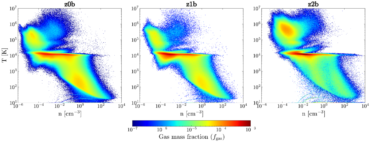
Figure 4. Refer to the following caption and surrounding text. — **Figure 4.** The temperature–density phase diagram of gas within R_vir at the end of the simulations. Despite the differences in redshift and environment, the distributions of gas density and temperature show similar patterns among all the simulations. Based on the temperature, the gas can be divided into three phases: the cold phase (T < 10³ K), the warm phase (T ∼ 10³–10⁴ K), and the hot phase (T > 3 × 10⁴ K). In each phase, the density and temperature show a log-normal distribution. Most of the gas in both the galaxy and the CGM resides in the warm phase, exhibiting a wide range of density distributions.
Download figure:
Standard image High-resolution image

To investigate the multiphase structure of the CGM, we plot the halo gas temperatures in Figure 5. Most of the gas in the galactic disk has a temperature of T ≲ 10⁴ K, and some cold gas can extend into the CGM. The distribution of the gas phases also depends on the redshift. For the CGMs of galaxies at z = 0 and z = 1, most of the gas is at T < 10⁵ K, with some filamentary structures of T ∼ 10⁴ K connected to the central galaxies. This picture is consistent with the cold accretion model (A. Dekel & J. Woo 2003). However, the CGM at z = 2 is dominated by hot gas. Inside the hot gas, a small fraction of cold gas forms a ring-shaped structure surrounded by the galaxy, which implies the tidal stripping of the cool ISM driven by the CGM accretion shown in Figure 4.

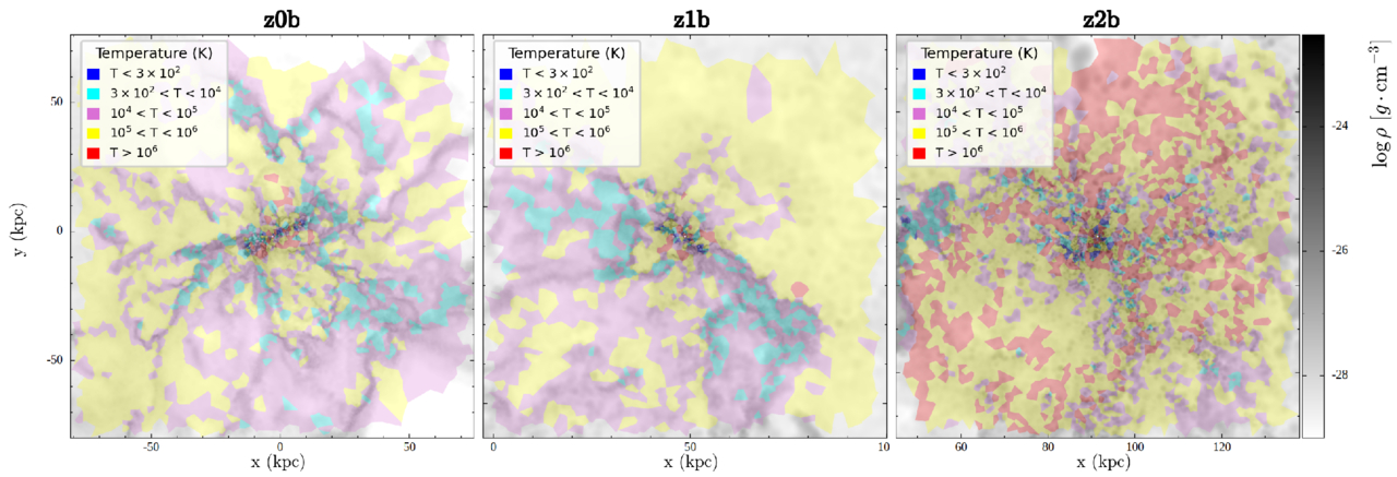
Figure 5. Refer to the following caption and surrounding text. — **Figure 5.** The temperature distribution of the halo gas at the end of the simulations on top of the gas density, in the gray color. We show the gas in five different temperature ranges: T < 300 K (blue), 300 K < T < 10⁴ K (cyan), 10⁴ K < T < 10⁵ K (purple), 10⁵ K < T < 10⁶ K (yellow), and T > 10⁶ K (red). The patchy color distribution of the temperatures and density clumps suggests the highly complex multiphase structure of the CGM.
Download figure:
Standard image High-resolution image

We further estimate the t_ff and t_c of our models, to decide whether the accretion is in the hot or cold mode. t_ff and t_c are estimated by

Equation or symbol description not available

where ρ and T are the averaged temperature and density of the CGM. The average gas cooling rate is assumed to be Λ ∼ 10⁻²² erg cm³ s⁻¹, based on the cooling curves from U. Maio et al. (2007). With the temperatures and densities from our models, t_ff roughly ranges from 500 to 1500 Myr and decreases with redshift, while t_c ranges from 50 to 1000 Myr, except for z0a, where t_c approaches 1500 Myr due to the low-density CGM. For each model, t_c < t_ff suggests that cold accretion dominates in these DGs. In addition, the ratios of cold to hot gas (separated by 3 × 10⁴ K) inside the CGMs are 1.04 (z0a), 3.31 (z0b), 0.98 (z1a), 4.3 (z1b), 5.78 (z2a), and 1.84(z2b). These results further support cold gas dominating the gas inflow, which is in agreement with the theoretical predictions from previous studies. The CGM at z = 2 remains cold-gas-dominated in mass, despite a large spatial covering fraction of hot gas. However, the fraction of accreted cold gas still varies, depending on the local environment. For instance, the isolated environment of z0a and the tidal stripping by a nearby massive galaxy in z1a can reduce the cold-gas accretion, leading to a lower cold-gas fraction.

3.2. Gas Accretion of the IGM and CGM

The coevolution of a galaxy and its CGM is critically determined by the accretion of the CGM and the outflow from the galaxy driven by the stellar feedback and AGN activity. We present the gas accretion and outflow history for the galaxies and CGMs in Figure 6. The evolution of the CGM accretion depends on the redshifts. At z = 0, the accretion rate is relatively steady. The weak outflow from the halo in z0a results from the limited gas supply from an isolated environment. On the other hand, z0b maintains a stable accretion rate from the cold accretion of filaments. For galaxies, their gas accretion rate varies significantly with time, especially at the galactic scale during the first 900 Myr. For the scale of ≥R_vir, the gas outflow exceeds the gas accretion most of the time. Furthermore, we find that the accretion rates of the galactic-scale region and the halo-scale region show a trend of anticorrelation for z1a, z1b, and z2b in Figure 6. The galactic disks in z2a and z2b show the strongest gas accretion rate, with a peak value around 10 times higher than those at z = 0 and z = 1. Again, the accretion rates vary significantly with time. The accretion and outflow rates fluctuate between 10 and −10 M_⊙ yr⁻¹. Unlike galaxies at z = 1, the accretion rates at galactic and halo scales are correlated, but with a time offset.

Figure 6. Refer to the following caption and surrounding text. — **Figure 6.** The evolution of the mass accretion rates during the simulations. We calculate the mass accretion rate by the temporal variation of the enclosed mass of the galactic disk scale within <0.2 R_vir (blue solid line) and of the halo scale of R_vir (orange dashed–dotted line), along with the reference of $\dot{M}=0$ (black dashed line). This mass accretion includes both the mass inflow and outflow of the targeted scale. Therefore, a positive accretion rate means the inflow mass is larger than the outflow, and a negative accretion rate shows that the inflow mass is smaller than the outflow. For all models, the accretion rate at a galactic disk scale of 0.2 R_vir is overall positive, indicating the growth of the galaxy with continuous gas fueling. In contrast, the mass accretion rate at R_vir can be negative, due to strong outflows. The accretion of the z = 1 and z = 2 models demonstrates significant variation at both the galactic disk scale and halo scale.
Download figure:
Standard image High-resolution image

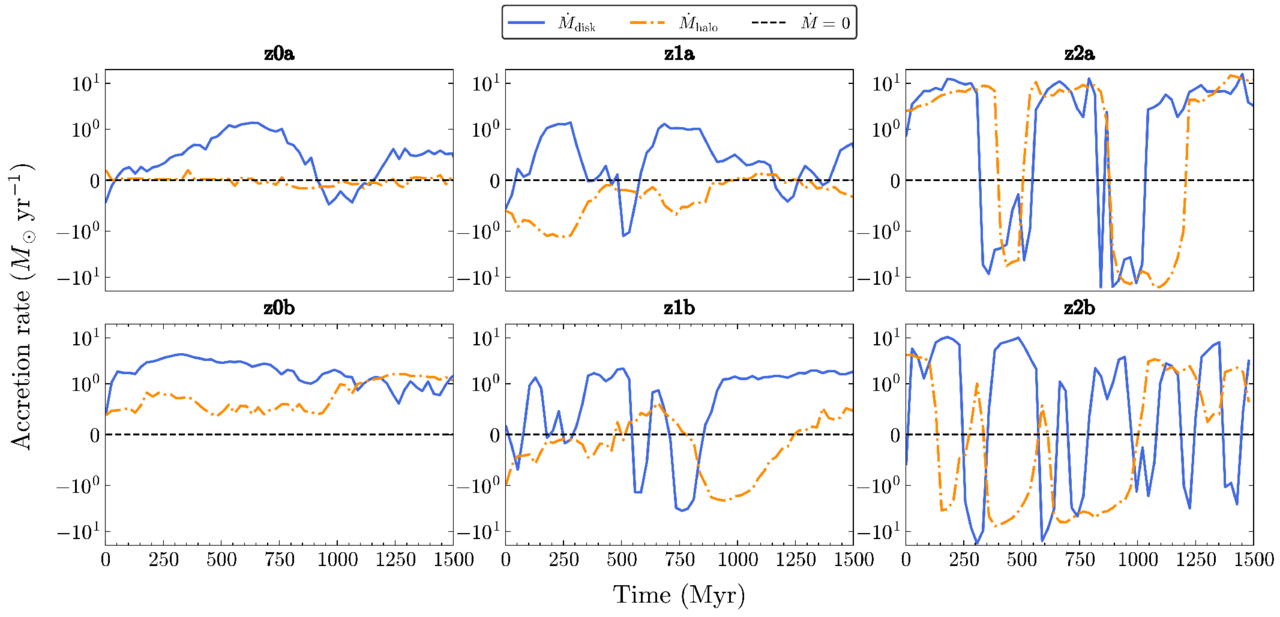
**Figure 6.** The evolution of the mass accretion rates during the simulations. We calculate the mass accretion rate by the temporal variation of the enclosed mass of the galactic disk scale within <0.2 R_vir (blue solid line) and of the halo scale of R_vir (orange dashed–dotted line), along with the reference of $\dot{M}=0$ (black dashed line). This mass accretion includes both the mass inflow and outflow of the targeted scale. Therefore, a positive accretion rate means the inflow mass is larger than the outflow, and a negative accretion rate shows that the inflow mass is smaller than the outflow. For all models, the accretion rate at a galactic disk scale of 0.2 R_vir is overall positive, indicating the growth of the galaxy with continuous gas fueling. In contrast, the mass accretion rate at R_vir can be negative, due to strong outflows. The accretion of the z = 1 and z = 2 models demonstrates significant variation at both the galactic disk scale and halo scale.
Download figure:
Standard image High-resolution image

The differences in the accretion rates result from the combined effects of redshifts, environments, and feedback, as shown in Figure 6. For DGs at higher redshifts, their surrounding CGM and IGM densities are higher, naturally leading to higher accretion rates. The DG halos at z = 2 achieve the highest accretion rates. In contrast, at z = 1, galaxy clustering substantially affects our target DG halos at the CGM scale, suppressing the cold-gas inflow from both the CGM and the IGM. Additionally, lower-mass galaxies exhibit more bursty SF compared to higher-mass galaxies (D. R. Weisz et al. 2012). Our z = 1 models represent an evolution path, transiting between the high accretion rates from z = 2 to z = 0. During this regime, galactic-scale gas inflow influences halo-scale accretion after a delay, due to episodic SF and subsequent stellar feedback. Such delayed interactions create an anticorrelation between the accretion rates at halo and galactic scales. A similar phenomenon is also observed during the early evolution of z2b. Notably, among all the models, the z0b model exhibits the highest average net accretion rate, primarily driven by its steady gas inflow and relatively weak outflows.

3.3. Metallicity of Galaxies and Their CGM

We examine the chemical properties of DGs and their CGM by presenting their absolute metallicity⁴ distribution in Figure 7. In z0a, the metal-rich gas of the galaxy is smoothly mixed and diffused into its CGM. The CGM at z = 0 shows a distinct drop in metallicity in the outer regions, consistent with observations (R. Bordoloi et al. 2014). However, for the other redshifts, the metal is widely distributed throughout the entire CGM, implying strong galactic outflows that chemically enrich the CGM. Furthermore, the CGM in the z = 2 models shows clumpy structures in the metal distribution, due to the mixing of metal-rich gas ejected from the central galaxies and metal-poor gas accreted from the IGM. Some ejected gas clumps, containing metal-rich SN ejecta, can reach a higher metallicity than the disk gas (C. R. Christensen et al. 2018).

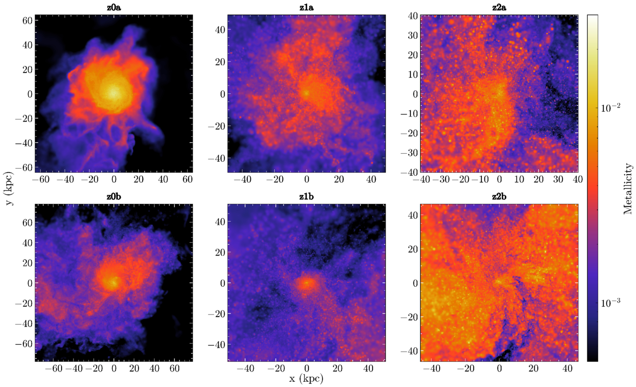
Figure 7. Refer to the following caption and surrounding text. — **Figure 7.** The metallicity distribution of halo gas at the end of the simulations. The metal distribution in the z = 2 halos is more extensive than that of the z = 0 and z = 1 halos.
Download figure:
Standard image High-resolution image

We show the evolution of the 1D metallicity profile in Figure 8. In the evolution of the metallicity profiles, the overall metallicity of z0b gradually increases over time. The metallicity profiles of z = 1 and z = 2 eventually become nearly uniform at r > 10 pc, suggesting efficient metal mixing in the CGM. The shallower gravitational potential of DGs allows them to eject more metal-rich gas from SNe into the CGM than more massive galaxies (C. R. Christensen et al. 2018). At the end of the simulations, the metallicity at the halo boundary increases by a factor of 2–3 from the beginning. However, in z1b and z2b, the metallicity distribution decreases within 10–20 kpc from 750 to 1500 Myr, due to the strong outflow driven by stellar and AGN feedback that transports the inner metal outward (see Figure 6).

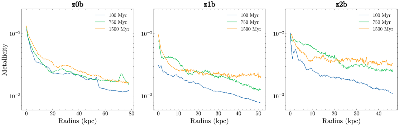
Figure 8. Refer to the following caption and surrounding text. — **Figure 8.** The radial metallicity of halos. The peak metallicity appears in the halo center below the solar metallicity of 0.02. The increasing CGM metallicity is from the metal produced in the star-forming region that is further transported to the entire halo by SNe and AGNs.
Download figure:
Standard image High-resolution image

The average metallicity of most DGs increases by 30%, and their corresponding total metal mass increases by a factor of 1.5–3 at the end of the simulation—although the metallicity of z0a decreases by about 14%, due to the dilution by accretion of metal-poor gas and weaker SF activity. On the other hand, z2b shows the smallest increase of total metal mass, by ∼10%, due to the strong stellar feedback that ejects much newly synthesized metal.

3.4. Dark Matter Mass and Structure

To study the dynamics of galaxies, we compare the distribution of dark matter for all models in Figure 9. The structure of the dark matter halo varies between redshifts. The halo exhibits a virialized spherical distribution in z0b. In contrast, the dark matter halos of z1b and z2b are more elongated. Moreover, several dense clusters of dark matter (the scattered little red dots for z2b in Figure 9) orbit around the halo center in z2b, suggesting minor mergers of tiny dark matter halos. These mergers may influence the evolution of the host galaxy via their tidal interactions.

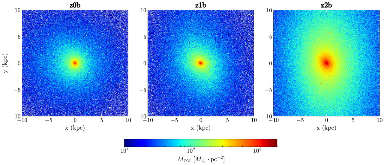
Figure 9. Refer to the following caption and surrounding text. — **Figure 9.** The inner dark matter structures of halos at the end of the simulations. These structures look spherical, and their radial profiles follow Navarro–Frenk–White profiles (J. F. Navarro et al. 1996). In z2b, several little red dots are scattered around the outskirts of the halo center, possibly due to the minor merger of the surrounding mini halos.
Download figure:
Standard image High-resolution image

3.5. The Growth of SMBHs

To evaluate the impacts of SMBHs on DGs, we show the history of the accretion rate for the SMBH in Figure 10. Most of the SMBHs exhibit quasiperiodic outbursts in their accretion rate history, implying the short duration of the active duty cycle. The highest SMBH accretion rate occurs in z2a, at 1000 Myr, surrounded by several smaller bursts with a time separation of ∼100 Myr. The peak rates of z2a and z2b can reach ∼10% of the Eddington accretion rate,

where M_6,BH is the mass of the SMBH in units of 10⁶ M_⊙. This AGN activity also leads to intense feedback on the CGM, by blowing the metal-rich gas away from the galaxy into the CGM and creating a strong outflow.

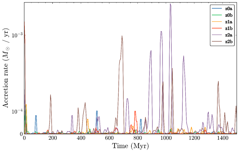
Figure 10. Refer to the following caption and surrounding text. — **Figure 10.** The accretion history of the SMBH throughout the simulation. The accretion histories show a bursty pattern for the z = 1 and z = 2 models, suggesting several duty cycles of AGN activity and the rapid growth of the SMBHs. The peak accretion rates reach ∼10% of the Eddington rates.
Download figure:
Standard image High-resolution image

As discussed in Section 3.2, the galaxies’ high gas accretion rate possibly triggers the busty accretion of the SMBH. For z2b, the SMBH accretion is primarily driven by the gas accretion from filamentary CGM structures. Meanwhile, part of the accretion in z2a is from the minor mergers of smaller surrounding structures. For a gas-rich galaxy, such as z0a, the SMBH activity can be triggered even without a high accretion rate from CGM. Compared with z0a and z0b, the SMBH accretion rate in z0b is lower, despite its higher CGM accretion rate.

3.6. SF

We show the evolution of the SFRs of all models in Figure 11. In general, the gas accretion rate from the CGM is sufficient to sustain the SFR for galaxies among all redshifts. However, minor mergers and stellar and SMBH feedback also affect the galactic SFR and are reflected in the gas accretion rates, as shown in Figure 6. For z0a and z0b, the evolutionary track of the SFR is steady and increases slightly during the simulations. Moreover, the more compact stellar disk can survive under the strong SMBH feedback and accretion flow, as shown in Figures 6 and 10.

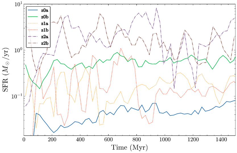
Figure 11. Refer to the following caption and surrounding text. — **Figure 11.** SFR histories for all models. The DGs at z = 1 and z = 2 show bursty SFH, with variations spanning a range of 2 dex, as also found in S. Shen et al. (2014). As z increases, the average SFR in the DGs also increases.
Download figure:
Standard image High-resolution image

For z1a and z1b, their average SFR is lower than that of z0b. Because the gas accretion of z1a and z1b is subject to tidal interactions from their distant neighbors—massive galaxies—affecting the CGM and surrounding IGM, it causes a drop in the accretion rate of the CGM and IGM. The SFR also exhibits larger variability during the first 100 Myr, then becomes more steady, which correlates well with the gas accretion rate around the galactic scale. This behavior is also related to the rapidly evolving structure of the gas disk and dark matter halo.

For the galaxies at z = 2, their SFRs are 10–100 times higher than those of the galaxies at z = 0 and z = 1. The high accretion rate and irregular shape of the galaxy allow cold gas to flow directly into the center, boosting SFRs while simultaneously increasing outflows, due to feedback from stars and the SMBH, leading to a rapid variation in SFR. The dynamic impact of the strong inflows from the CGM and minor mergers can also alter the structure of the galactic disk and its SFR.

We further examine the correlation between the SFE and other physical quantities in Figure 12. The SFE is more sensitive to redshift than to the amount of star-forming mass and the molecular gas fractions of DGs. The left panel of Figure 12 shows that the SFE increases as z increases and the SIMBA simulations (R. Davé et al. 2019; L. Ghodsi et al. 2024) also found similar results. The middle and right panels of Figure 12 show weak correlations between the SFE and star-forming gas mass and fraction. This result demonstrates that z has a stronger impact than the halo properties of DGs on their SFEs.

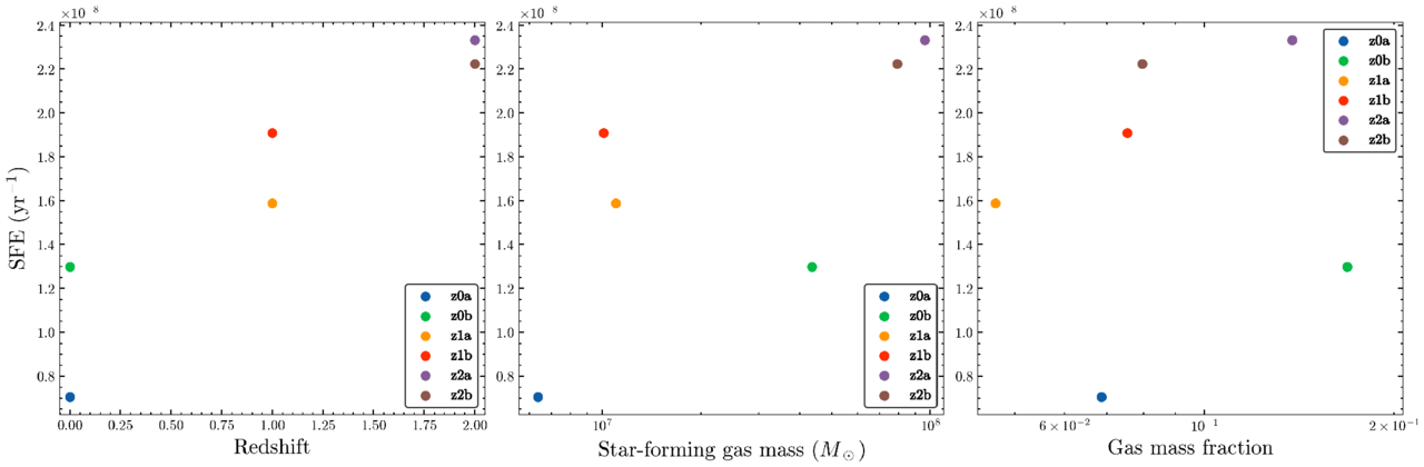
Figure 12. Refer to the following caption and surrounding text. — **Figure 12.** The SFEs with respect to redshift (left), star-forming gas mass (middle), and gas mass fraction within DG halos (right). The amount of star-forming gas mass is the sum of the molecular mass of the gas density at >0.1 cm⁻³. The SFEs have a stronger correlation with redshift than with the amount of star-forming gas mass and the gas mass fraction inside the halo.
Download figure:
Standard image High-resolution image

3.6.1. Spatial Distribution of SF Region

We show the stellar disk structure of the DGs in Figure 13. The SF regions become more compact both in the gas disk and in the bulge as z increases. In z1b, due to the unstable structure and the pulsational outflows of the galactic disk, the SF region appears to be more elliptical or bulge-dominated. In z2b, with a continuous gas supply and high gas density, the SF region is populated throughout the disk, with the peak at the center. The clumpiness of the SF density is likely generated by the disk instability via strong accretion. Combined with the SMBH accretion rate in Section 3.5, both explain why the strong accretion flow on the galactic scale at z = 2 can effectively reach the galactic center, triggering both active SF and SMBH activity.

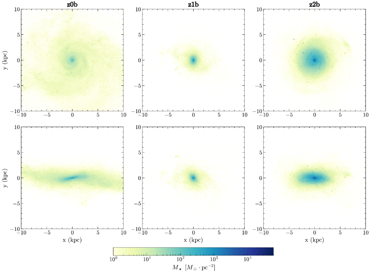
Figure 13. Refer to the following caption and surrounding text. — **Figure 13.** The spatial distribution of the stars formed within the inner region of 5 kpc at the end of the simulation. The top and bottom panels show the face-on and edge-on views of the galaxies, respectively. Among these models, only z0b shows a spiral structure. In z2b, some scattering SF regions appear at the outskirts of the disk, due to the SF in the clumpy disk. This clumpy structure may be driven by disk instabilities via the strong gas accretion from the CGM.
Download figure:
Standard image High-resolution image

4.1. The Metal Enrichment of the CGM

The cooling of hot gas by metals through line emission is efficient. Therefore, the metal content of the CGM can affect the evolution of the galaxy and its CGM. Furthermore, the metals ejected from the galaxy can serve as a tracer in the CGM to probe the coevolution of the galaxy and the CGM. In Section 3.3, we examine the spatial distribution of the metallicity and its temporal evolution. To evaluate the mixing within the simulation box, we present the kinetic energy spectra of the gas in Figure 14, based on the snapshots in Figure 8. For all halos, the slope of the power spectra is −5/3, aligning well with the Kolmogorov spectra (V. E. Zakharov et al. 1992; J. Scalo & B. G. Elmegreen 2004). This result suggests that the gas within the halo scale is highly turbulent.

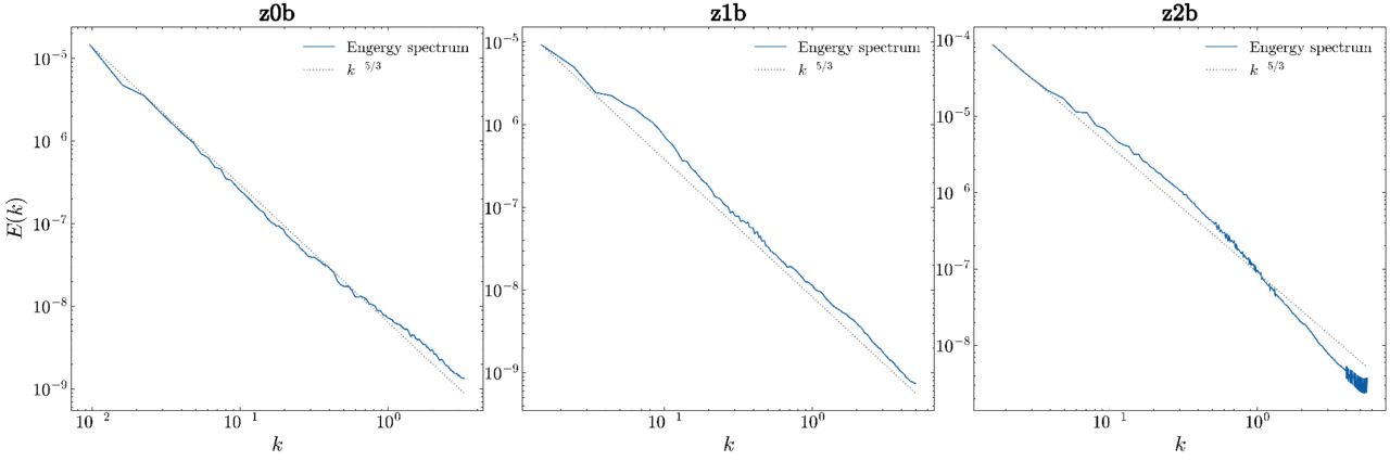
Figure 14. Refer to the following caption and surrounding text. — **Figure 14.** Kinetic energy power spectrum of the halo gas at the end of the simulation. The slopes of the gas spectra match well with the dotted line, presenting the slope of −5/3 for the typical Kolmogorov spectrum. These profiles suggest that the entire halo gas is highly turbulent.
Download figure:
Standard image High-resolution image

Large-scale mixing is driven by interactions between the halo inflows and galactic outflows. This mixing can disperse metal from galaxies to the CGM efficiently. Furthermore, the gas inflow rates determine the SF and consequent stellar feedback. Therefore, the inflow influences the total metal mass within the galaxies. For z2b, the slope of the spectrum becomes slightly steeper than −5/3 at large k, indicating weaker turbulence on the small scale. This may result in insufficient mixing of the gas clumps ejected from the DGs, as shown in Figure 7, in contrast to the well-mixed CGM at lower-redshift galaxies suggested by Z. Hafen et al. (2019). However, strong stellar and SMBH feedback can still transport metals in z2a and z2b to the halo boundary or beyond, as shown in the metallicity distribution profiles of Figure 8.

4.2. The Impact of the Evolved CGM and IGM Gas on Host Galaxies

We now quantify the mass of the accreting gas during the evolution and discuss its impact on the SFR and the gas mass evolution of the galaxy and halo. By tracing the gas in the simulations as shown in Figure 15, we can follow the gas evolution of the galaxy, CGM, and IGM, as well as their contributions to SF. We label each gas particle at 100 Myr, to allow some relaxation time after splitting the gas particles. We then track these particles until the end of the simulation at 1500 Myr. Furthermore, we can calculate the mass change rates for gas originating from the galaxy, CGM, and IGM separately, unlike the total mass change rate of the enclosed mass with a given region, as shown in Figure 6.

4.2.1. SF

The left panel of Figure 16 shows the contribution of the star-forming gas from the galaxy, CGM, and IGM. In general, the contributions of the galaxy, CGM, and IGM depend on z. The original gas residing in the galaxy accounts for ∼70% of the star-forming gas for galaxies at z = 0 and ∼50% for galaxies at z = 1. The value drops further as the redshift increases. At z = 2, the gas originating from the galaxy contributes only <20% to the SF gas. The strong accretion and outflow for high-z galaxies cause the initial galactic gas to become a subdominant component in the SF.

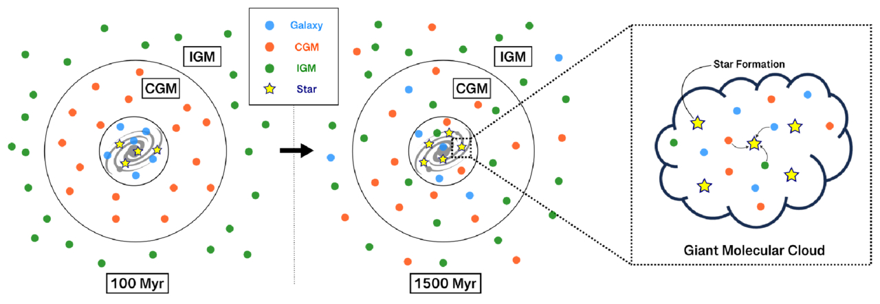
Figure 15. Refer to the following caption and surrounding text. — **Figure 15.** Schematic of the gas particle tracing. The blue, orange, and green dots represent the gas particles initially from the galaxy, CGM, and IGM, respectively, at the beginning of the simulations. The middle panel shows the gas distribution at the end of the simulation, where the colored dots are mixed, due to the gas accretion and outflow. The right panel shows a close-up of the SF region within the galaxy. Gas accreted from the CGM and IGM partially contributes to the SF within the galaxy.
Download figure:
Standard image High-resolution image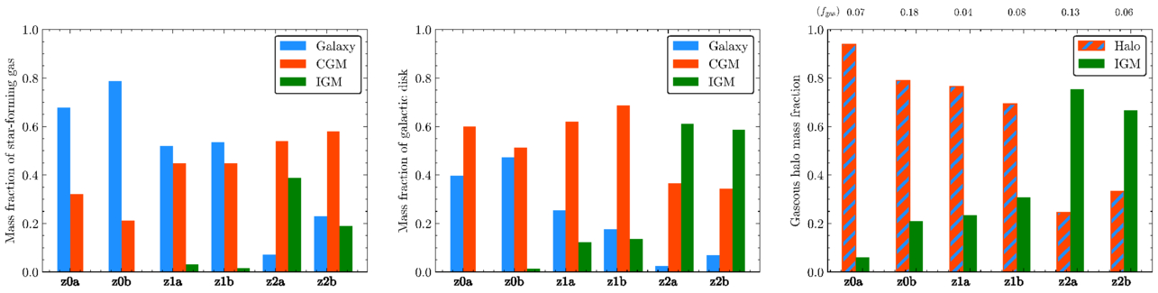

Figure 16. Refer to the following caption and surrounding text. — **Figure 16.** The gas contribution from the original galaxy, CGM, and IGM to the star-forming gas (left), galactic disk (middle), and halo gas (right) at the end of the simulation. The orange bars with blue stripes in the right panel represent the total gas mass inside a halo, including galaxy and CGM gas. These contributions are calculated using a particle-tracking technique, by tagging each gas particle and following its trajectory until its final destination. The gas mass fraction of the entire galactic halo (f_gas) is added on top of the gaseous halo plot.
Download figure:
Standard image High-resolution image

Meanwhile, the gas contribution to the SFR from the CGM and IGM increases with redshift. The accreted CGM gas dominates the mass in the reservoir of SF, from 20% of gas for z = 0 galaxies to 50% for z = 2 galaxies. For the contribution from the IGM, it is much more sensitive to the redshift, from 0. 01% to 20%, when z increases from 0 to 2. The influence of the IGM is minor for galaxies at z = 0 and 1. However, the evolution of z > 2 galaxies should include their IGM. In sum, our results demonstrate the importance of the CGM and IGM for the evolution of high-z galaxies.

4.2.2. Mass and Structure of Galaxy

In the middle panel of Figure 16, we present the contribution of the gas inside the galaxy, defined as the gas with a distance from the central SMBH of less than 0.2R_vir. The result is different from the contribution of SF. During the 1.5 Gyr simulation, the CGM and IGM gas can eventually contribute >50% of the gas inside the galaxy, even for z0a, having minimal environmental accretion beyond the halo scale. This suggests that the CGM plays a critical role in the galaxy’s evolution across cosmic time. The contribution of gas from the CGM can account for around 40%–70% of the total gas mass in the galaxy. Furthermore, it should be mentioned that the effect of the CGM is more important at z = 1 (70%). For the contribution of the IGM to the galactic gas, the percentage increases from z = 0 to z = 2 and reaches 60% at z = 2, surpassing the CGM.

4.2.3. Halo Mass and Size

In the right panel of Figure 16, we present the contribution of the total gas mass inside the halo of <R_vir. The mass fraction contributed by the IGM to the halo mass differs between redshifts. For z = 0 and z = 1, except for the isolated galaxy z0a, the IGM can contribute 20%–30% of the total gas mass inside the halo after 1.5 Gyr of evolution. For the z = 2 galaxies, the contribution of the IGM can account for 60%–70% of the gas in the halo, dominating the entire gas reservoir over the galaxies and CGM in the early Universe.

4.3. Comparison to Previous Studies and Observations

R. Bordoloi et al. (2014) suggested that the total carbon mass within a DG is comparable to that in its CGM at z ∼ 0, which is consistent with the metallicity results of our simulations. We present the accumulated metal mass fraction as a function of the radius within a halo in Figure 17. The profiles vary significantly between the z = 0 and z = 2 halos. These differences relate to two different modes of metal enrichment. At z = 0, a steeper metallicity gradient between the galaxies and their CGM appears, due to the weaker stellar and AGN feedback. Furthermore, z0a and z0b can be explained by the “three-zone” structure—of galaxies, the inner CGM, and the outer CGM—as proposed in F. Li et al. (2021), and they also agree with observational metal detections found within the half-virial radius for DGs at z < 0.3 (Y. Zheng et al. 2024). However, the feedback is much stronger at z = 2, due to active SF and SMBH accretion. This drives a strong outflow containing metal-rich gas from galaxies to the CGM and smoothens the galaxy–CGM metallicity gradient. The flow driven by stellar and AGN feedback plays a crucial role in transporting the metal from galaxies to their CGMs (A. Dekel & J. Silk 1986; L. V. Sales et al. 2022). For high-redshift galaxies, stronger outflows can ship galactic metals to the CGM and even to the IGM. For the CGM region, the models of the larger-virial-mass models of z0b, z1b, and z2b have a higher metal fraction than the models of z0a, z1a, and z2a at a given r. We summarize the SFR and gas accretion rates contributed by the initial galaxy, CGM, and IGM in Table 2. DGs of higher virial mass have higher SFR and gas accretion rates that apply to the models of z = 0 and z = 1. Furthermore, in Figure 17, halos with a higher virial mass exhibit a higher metal fraction in CGM at z < 2.3

Table 2. The Averaged Rates of Star-forming Gas ( ${\dot{M}}_{\star }$ ), Disk Gas ( ${\dot{M}}_{\,\rm{Disk}\,}$ ), and Halo Gas ( ${\dot{M}}_{\,\rm{Halo}\,}$ ) Contributed by the Initial Galaxy, CGM, and IGM

Model Name	${\dot{M}}_{\star }$				${\dot{M}}_{\,\rm{Disk}\,}$			${\dot{M}}_{\,\rm{Halo}\,}$
	(M_⊙ yr⁻¹)				(M_⊙ yr⁻¹)			(M_⊙ yr⁻¹)
	(Galaxy)	(CGM)	(IGM)	(Total)	(CGM)	(IGM)	(Total)	(IGM)
z0a	0.026	0.012	0.0	0.038	0.630	0.002	0.632	0.081
z0b	0.380	0.102	0.0	0.482	1.843	0.048	1.891	1.360

z1a	0.076	0.066	0.005	0.147	0.373	0.074	0.447	0.252
z1b	0.106	0.089	0.003	0.198	0.724	0.143	0.867	0.630

z2a	0.158	1.194	0.856	2.208	0.887	1.482	2.369	5.562
z2b	0.385	0.971	0.316	1.672	0.409	0.700	1.109	2.920

Download table as: ASCII Typeset image

Table 3. Physical Properties of DGs in Our Runs and TNG50-1

Model	SFR	M_⋆	M_gas	R_⋆,1/2	M_BH
	(M_⊙ yr⁻¹)	(10⁸ M_⊙)	(10⁸ M_⊙)	(kpc)	(10⁶ M_⊙)
z1a	0.36	2.46	3.15	1.28	1.75
z1a*	0.0078	1.44	0.44	2.22	2.45

z1b	0.18	4.38	0.016	0.8	1.60
z1b*	0.061	1.62	0.56	1.44	3.14

z2a	6.02	19.6	18.4	1.54	1.97
z2a*	0.69	4.93	4.33	3.88	3.87

z2b	4.35	16.2	6.59	1.24	1.86
z2b*	0.86	6.85	3.96	3.37	4.87

Note. We compare our simulated z = 1, 2 DGs with their original counterparts in TNG50-1 at the same epoch, corresponding to the z evolution from ≈2 → 1.3 and ≈1 → 0.4. The DGs in TNG50-1 are marked with an asterisk (*). Five physical quantities are listed: SFR, M_⋆, M_gas, R_⋆,1/2, and M_BH.

Download table as: ASCII Typeset image

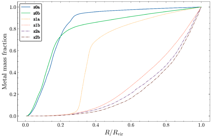
Figure 17. Refer to the following caption and surrounding text. — **Figure 17.** Profiles of an accumulated metal fraction within R_vir. For z0a and z0b, most of the metal resides in the galaxy, and their profiles start to diverge at 0.2–0.3 R_vir. Meanwhile, **z2a** and **z2b** show a different pattern, with most of the metal smoothly distributed around the CGM. The profiles of z1a and z1b fall between the z = 1 and z = 2 models. The metal fraction in z1b is closer to the distribution observed in the z = 2 models, while the profile of z1a appears as a transition between z0b and z1b. Such transitions in the metal distribution may be related to the coevolutionary stage of the DGs and their environments.
Download figure:
Standard image High-resolution image

Y. Zheng et al. (2024) found that only ∼10% of the metal in the whole halo exists in the warm phase (T ∼ 10⁴ K) of the CGM in low-redshift DGs, agreeing well with our results for the warm-phase metal, with 6% for z0a and 15% for z0b. Y. Zheng et al. (2024) also suggested that there is more metal in the warm phase as z increases. Meanwhile, our results show that the metal in the warm phase is 12% (z1a) and 20% (z1b) for z = 1, and 20% (z2a) and 14% (z2a) for z = 2.

In our simulations, the mass of the CGM over the baryonic mass of the halo is 16% (z0a), 38% (z0b), 35% (z1a), 42% (z1b), 50% (z2a), and 48% (z2b); it shows an increasing trend from z = 0 to z = 2, emphasizing the importance of the CGM gas at higher z, as shown in Figure 16. Our results also align with the results from Z. Hafen et al. (2019), based on FIRE collaborations (P. F. Hopkins et al. 2014, 2018b, 2023), suggesting that the CGM of 10¹⁰–10¹² M_⊙ halos contains ∼40%–70% of its baryonic mass at z = 2. The only outlier, z0a, shows a CGM mass fraction of 16%—a rare isolated environment, where most baryons are concentrated in the galaxy. In general, the mass fraction of the CGM gas in our models is slightly lower than the results of Z. Hafen et al. (2019). This discrepancy may arise from differences between the simulation setups, e.g., the initial conditions of the zoom-in runs and our semi-cosmological runs. Our TNG initial conditions contain stars formed before the simulations start, which may lead to higher stellar masses affecting the stellar feedback and gaseous halos. L. V. Sales et al. (2022) also suggest that differences between the models may result from more baryons accumulating inside the galaxy in cosmological simulations. For the gas mass alone, the CGM mass fractions over the total halo gas are 20%(z0a), 45% (z0b), 44% (z1a), 49% (z1b), 67% (z2a), and 72% (z2b) in our simulations.

Based on FIRE and FIRE2 simulations, Z. Hafen et al. (2019, 2020) suggest that ∼60%–80% of the CGM gas mass in 10¹⁰–10¹² M_⊙ halos is fueled by IGM accretion, which is consistent with our findings of 60%–70% from z2a and z2b.

4.4. Comparison with TNG50-1

The major difference between our models and their original counterparts in TNG50-1 is in their SF properties. In Table 3, our galaxies exhibit higher SFRs within a smaller SF region, resulting in smaller R_⋆,1/2. This discrepancy arises due to the combined effects of resolution, cooling, and subgrid SF modeling. The original TNG projects are designed to study the galaxy formation at z = 0 through cosmological simulations. Therefore, the ISM physics and SF processes are modeled with subgrid models with limited resolution, by utilizing an effective equation of state in the ISM (V. Springel & L. Hernquist 2003; M. Vogelsberger et al. 2013; P. Torrey et al. 2014). In contrast, our high-resolution simulations can resolve clumpy SF regions and consider the detailed gas cooling and chemistry that can better model the SF processes. Furthermore, the enhanced feedback from the higher SFR can create compact galactic disks, by evaporating the outer regions of less dense gas.

The BH accretion rates in our models and TNG are also different. The gas accretion rates in our models are lower, due to the weaker dynamical friction of the lower cell mass (C.-H. Lin et al. 2023). As shown in Figure 10, the accretion histories of our models show episodic and bursty patterns, due to the accreting of clumpy gas in the galactic centers. This accretion pattern agrees well with J. M. Gabor & F. Bournaud (2013) and C. DeGraf et al. (2017), demonstrating the effect of the simulation resolution in modeling BH accretion.

4.5. Limits of the Current Models

Although the resolution of the simulation is higher compared with previous galaxy simulations, we are still unable to resolve regions such as the SF sites, stellar feedback, and the accretion disk of the SMBH. Therefore, we employ subgrid models for SF and SMBH accretion, with the convergence of these models being carefully verified. Nevertheless, the modeling of the physics of stellar and SMBH feedback is still crude in the current simulations and has ample room to improve. Furthermore, we also adopt a local UV background for all of our simulations. This setup is a trade-off between maintaining the integrity of the local environment and accounting for the effect of UV photons originating from outside our target DG. However, a more realistic UV background involving the local radiative field is needed to properly model the evolution of the IGM and CGM.

We present new high-resolution simulations of DGs and their CGM/IGM across cosmic time, with initial conditions from a realistic cosmological simulation from IllustrisTNG. Our results show the complex multiphase gas of the CGM and IGM being driven by gas accretion, the SMBH, and stellar feedback from the host galaxies. We also tracked the accretion gas from the CGM and IGM, to quantitatively evaluate their impact on the evolution of galaxies. In general, the gas accreted from the CGM depends on z and plays a crucial role in fueling the gas reservoir and driving galactic SF. During 1.5 Gyr of evolution, the DGs grow solely through the accretion contributed by the CGM at z = 0 and z = 1. Overall, the CGM gas contributes 20%–50% to the total star-forming gas and 40%–70% to the gas mass of galaxies. At z = 2, the CGM and IGM contain 60%–70% of the total halo gas mass, and the consequent gas accretion from them further contributes ∼60% of the galaxy mass. The strong accretion flow from the IGM/CGM triggers intense AGN activity and active SF at the galactic center. Furthermore, the SMBHs of the DGs at z = 2 show episodic accretion histories, with a peak up to ∼10% of the Eddington mass accretion rate, indicating phases of rapid growth. Our results suggest the increasing importance of the coevolution of DGs and their CGM in a high-z Universe, which will possibly be examined by coming observations from JWST.

The authors appreciate Chorng-Yuan Hwang for his insightful discussions and thank Chi-Hung Lin, Kung-Yi Su, and Po-Feng Wu for their support of this work. This research is supported by the National Science and Technology Council, Taiwan, under grant Nos. MOST 110-2112-M-001-068-MY3 and NSTC 113-2112-M-001-028-, 114-2112-M-001-012-, and Academia Sinica, Taiwan, under a career development award under grant No. AS-CDA-111-M04. K.C. acknowledges the support of the Alexander von Humboldt Foundation and Heidelberg Institute for Theoretical Studies. This research was supported in part by the NSF PHY-2309135 grant to the Kavli Institute for Theoretical Physics (KITP) and by the NSF PHY-2210452 grant to the Aspen Center for Physics. Our computing resources were supported by the National Energy Research Scientific Computing Center (NERSC), a U.S. Department of Energy Office of Science User Facility operated under Contract No. DE-AC02-05CH11231, and the TIARA Cluster at the Academia Sinica Institute of Astronomy and Astrophysics (ASIAA).

Coevolution of Dwarf Galaxies and Their Circumgalactic Medium Across Cosmic Time

Authors

Article metrics

Share this article

Article information

Dates

Abstract

Related links

1. Introduction

2. Methodology

2.1. GIZMO Code

2.1.1. Hydrodynamics

2.1.2. Gas Cooling

2.1.3. SF and Stellar Feedback

2.1.4. SMBH Growth and Feedback

2.2. Simulation Setup

2.2.1. Initial Conditions from the IllustrisTNG Project

2.2.2. Resolution

3. Coevolution of DGs and Their CGM

3.1. Physical Properties of DGs and Their CGM

3.2. Gas Accretion of the IGM and CGM

3.3. Metallicity of Galaxies and Their CGM

3.4. Dark Matter Mass and Structure

3.5. The Growth of SMBHs

3.6. SF

3.6.1. Spatial Distribution of SF Region

4. Discussion

4.1. The Metal Enrichment of the CGM

4.2. The Impact of the Evolved CGM and IGM Gas on Host Galaxies

4.2.1. SF

4.2.2. Mass and Structure of Galaxy

4.2.3. Halo Mass and Size

4.3. Comparison to Previous Studies and Observations

4.4. Comparison with TNG50-1

4.5. Limits of the Current Models

5. Conclusion

Acknowledgments

Footnotes

Show References

2.1. `GIZMO` Code

2.2.1. Initial Conditions from the `IllustrisTNG` Project