Abstract
The AGN STORM 2 Collaboration targeted the Seyfert 1 galaxy Mrk 817 for a year-long multiwavelength, coordinated reverberation mapping campaign including Hubble Space Telescope, Swift, XMM-Newton, NICER, and ground-based observatories. Early observations with NICER and XMM revealed an X-ray state 10 times fainter than historical observations, consistent with the presence of a new dust-free, ionized obscurer. The following analysis of NICER spectra attributes variability in the observed X-ray flux to changes in both the column density of the obscurer by at least one order of magnitude (NH ranges from  to
to  ) and the intrinsic continuum brightness (the unobscured flux ranges from 10−11.8 to 10−10.5 erg s−1 cm−2). While the X-ray flux generally remains in a faint state, there is one large flare during which Mrk 817 returns to its historical mean flux. The obscuring gas is still present at lower column density during the flare, but it also becomes highly ionized, increasing its transparency. Correlation between the column density of the X-ray obscurer and the strength of UV broad absorption lines suggests that the X-ray and UV continua are both affected by the same obscuration, consistent with a clumpy disk wind launched from the inner broad-line region.
Original content from this work may be used under the terms of the Creative Commons Attribution 4.0 licence. Any further distribution of this work must maintain attribution to the author(s) and the title of the work, journal citation and DOI.
1. Introduction
Active galactic nuclei (AGN), formed by the accretion of gas onto a supermassive black hole, often surpass the total luminosity of their host galaxy despite their small relative size (Salpeter 1964). This energetic output has directly observable effects on the host’s evolution, as it can heat gas in the central region of the galaxy, potentially quenching star formation in a process known as AGN feedback (e.g., Hopkins et al. 2008; Fabian 2012; Tombesi et al. 2015; Baron et al. 2018). To better understand the origin of AGN feedback, we need a more robust understanding of AGN structure. Aside from a few notable exceptions such as M87 (Event Horizon Telescope Collaboration et al. 2019) and NGC 3783 (GRAVITY Collaboration et al. 2021), spatially resolved observations of inner AGN structure have been unattainable, so indirect measurements are required.
Reverberation mapping is one such indirect technique, in which AGN geometry is probed by tracking the delays, or lags, in the response of the accretion disk continuum and emission lines to variable ionizing radiation (see Cackett et al. 2021 for a recent review). In the X-ray reprocessing scenario, these delays are attributed to the light-crossing time of X-rays emitted by a compact corona near the supermassive black hole, which irradiates the accretion disk (e.g., Cackett et al. 2007). For a geometrically thin, optically thick disk (Shakura & Sunyaev 1973), the hottest innermost region of the disk is expected to respond first in the UV, with an increasing delay in the near-IR/optical response of the cold outer disk corresponding to the disk’s size.
The X-ray reprocessing scenario has been challenged by the poor correlation between observed X-ray and UV/optical variability in several sources (e.g., Edelson et al. 2019). In some sources, including Mrk 817 (Morales et al. 2019; Kara et al. 2021, E. Cackett et al. 2023, in preparation, hereafter Paper IV), no significant correlation between the X-ray and UV is observed. These studies rely on Swift XRT observations for X-ray variability and are thus limited to observing trends in the broadband X-ray flux, as Swift count rates are too low to reliably model contributions from individual X-ray spectral regions in AGNs (see Figure 1).

Figure 1. Count rate X-ray spectra taken on 2020 December 25. NICER XTI (purple circles; 1.1 ks exposure) observes Mrk 817 at a ∼20 × higher count rate than Swift XRT (green squares; 892 s exposure).
Download figure:
Standard image High-resolution imageThe AGN STORM 2 project is a large-scale, coordinated spectroscopic and photometric monitoring campaign designed to detect reverberation and gas dynamics across an entire AGN, Mrk 817, using X-ray through near-infrared observations from space- and ground-based observatories (Kara et al. 2021, hereafter Paper I). NICER monitoring was included to test the X-ray reprocessing scenario, due to its comparable scheduling flexibility to Swift and higher count rate sensitivity by a factor of ∼20. NICER, an array of 56 X-ray concentrators paired with silicon drift detectors, performs photon counting spectroscopy and timing measurements from its orbit aboard the International Space Station (Gendreau et al. 2012) over the energy range of 0.2–12 keV. The high count rates of NICER spectra enable physically motivated spectral modeling for each observation, including the individual contributions of the coronal continuum (Haardt & Maraschi 1991), the soft excess (Crummy et al. 2006), and obscuration from within the AGN (Reeves et al. 2008). By producing light curves for each emission component, lag-correlation tests can be conducted with coordinated UV/optical observations to identify the source of X-rays irradiating the disk.
Mrk 817 was initially selected for observation owing to its historically unobscured nature (Winter et al. 2011), in order to avoid complications to our spectral model from obscuring winds such as those seen in NGC 5548 (Dehghanian et al. 2019a, 2019b). However, as detailed in Paper I, observations of Mrk 817 with Swift and NICER in 2020 revealed a heavily extinguished soft X-ray state, and follow-up XMM observations confirmed the presence of a dust-free, ionized obscurer. Separate analysis of a concurrent NuSTAR observation also demonstrated the highly obscured state of Mrk 817 (Miller et al. 2021).
In Paper I, early NICER data were grouped into five epochs and fit using the XMM obscurer model. Variability in the observed X-ray flux was shown to be primarily driven by changes in the hydrogen column density (NH, including both neutral and ionized hydrogen) of the obscuring gas. These changes in NH were correlated with changes in the UV obscuration measured using the Cosmic Origins Spectrograph(COS) on board the Hubble Space Telescope, suggesting a common origin.
Models of the UV absorbers place them near the UV broad-line region (BLR) and the outer accretion disk at a distance of a few light-days from the black hole (Paper I). The outflow of clumpy material inferred from changes in NH suggests the presence of a disk wind, in which material from the accretion disk is launched outward. This also provides an explanation for the UV “broad-line holiday” early in the campaign, in which the observed correlation between the UV continuum and UV broad lines decoupled while the NH of the outflowing material was highest, similar to the wind-driven “holiday” observed in NGC 5548 (Dehghanian et al. 2019a).
In addition to their effects on the ionizing spectral energy distribution incident on the outer parts of the disk and BLR, disk winds have been considered as a potential mechanism for AGN feedback. Numerical calculations of radiatively driven (Dannen et al. 2019; Giustini & Proga 2019), thermally driven (Mizumoto et al. 2019; Waters et al. 2021), and MHD-driven winds (Fukumura et al. 2015, 2018) produce different outflow velocities, suggesting a range of significance for disk winds as feedback mechanisms. Observationally validating the impact of disk winds and assessing their acceleration mechanisms requires measurements of the line-of-sight covering fraction, NH, and the velocity of the outflowing material (Davies et al. 2020; Laha et al. 2020).
In this paper, we measure variability in the covering fraction and NH of the X-ray obscurer, presumably a disk wind, in Mrk 817 using individual NICER observations. These open a new doorway for testing time-dependent photoionization models of warm absorbers, such as those proposed by García et al. (2013), Proga et al. (2022), and Sadaula et al. (2022), by measuring the effect of X-ray source variability on the ionization of the obscuring gas.
The NICER data reduction techniques are discussed in Section 2. A detailed discussion of NICER background modeling is given in the Appendix. The spectral analysis is detailed in Section 3. In Section 4 we provide analyses of the variability seen in both the obscurer and the unobscured source. These are discussed in Section 5 and summarized in Section 6.
2. Observations and Data Reduction
NICER monitoring of Mrk 817 began on 2020 November 28 (hereafter Day 9181), 43 with an approximate cadence of 2 days as part of a TOO request (PI: E. Cackett, Target ID: 320186), and continued with observations from GO proposal 4128. The data were processed using NICER data analysis software version 2021-07-30_V008a (Blackburn 1995) and caldb version xti20210707 with the energy scale (gain) version 20170601v007. Event files were filtered using the standard nicerl2 settings excluding two noisy detectors, FPM 14 and 34. We excluded observations with a total exposure time of <400 s, leaving 183 epochs. Each spectrum was binned using the “optimal binning” scheme (Kaastra & Bleeker 2016) with a minimum of 25 counts per bin, using the FTOOLS module ftgrouppha.
We compared all three publicly available methods for estimating the NICER background (see the Appendix). Each estimator constructs a background using specific environmental and instrumental parameters as proxies for the background strength and spectral shape using data recorded during empty sky observations. The “Space Weather” estimator (K. Gendreau et al. 2023, in preparation) uses the angle between the Sun and the target, the magnetic cutoff rigidity due to the detector’s position in orbit, and the planetary Kenziffer index, which is a measure of current global geomagnetic activity (Bartels et al. 1939). The “3C50” estimator uses two instrumental parameters to assess whether detected photons are out of focus and thus associated with the background. A third noise parameter accounts for optical loading during the ISS day, in which the electrons freed by incident optical photons accumulate in the detector and produce a false signal, typically below 0.3 keV. Background-subtracted 3C50 spectra are subject to Level 3 filtering as defined by Remillard et al. (2022). The “Machine Learning” estimator classifies the background for each second of observation into one of 50 basis spectra derived from NICER observations of sky regions containing no X-ray sources. This model uses 40 parameters, including the six used by the 3C50 and Space Weather estimators (A. Zoghbi 2023, in preparation). 44
The X-ray source is highly extinguished by the obscurer below 3 keV, where NICER’s sensitivity is greatest. This necessitates a conservative filtering approach that excludes the background-dominated spectra most greatly affected by errors in the background estimation process. To minimize contributions from optical loading and the high-energy particle background, the energy range for all spectral analysis was restricted to 0.4–8 keV (rather than NICER’s full 0.2–12 keV sensitivity range). All three estimators produce comparable background-subtracted light curves in this energy range, with the best performance by the 3C50 method (see the Appendix), so these are used in subsequent analysis. We also remove 30 observations with a total 0.4–8 keV background of >1 counts s−1, because systematic uncertainties between the background estimators become significant above this threshold (Appendix). The mean background rate of the remaining observations is 0.55 counts s−1 (median 0.58 counts s−1), while the mean background-subtracted 0.4–8 keV source count rate is 1.75 counts s−1 (median 1.48 counts s−1), with a range of 0.75–9.96 counts s−1.
We explain the spectral shape of Mrk 817 using the absorbed power-law model introduced in Paper I, which was validated using XMM, NuSTAR, and NICER observations. It is fully described in Section 3.1. Observations where our standard model yields  are considered to be contaminated by an improperly modeled background. This
  cutoff excludes two additional observations, or 1% of the remaining epochs. The normalization of the coronal continuum, modeled using relxillD (García et al. 2016), is allowed to vary between 10−5 and 10−4 (Table 1). A total of 13 observations whose best-fit normalizations are driven to these limits are excluded from analysis. Those at the lower limit lack sufficient signal above 2 keV to constrain the power law properly. Those at the upper limit exhibit a very hard spectrum above 6 keV, in excess of the power-law source model from Paper I. This excess is characteristic of interference from the particle background, which has a much harder spectrum than the source.
Table 1. Model Parameter Constraints
| Component | Parameter | Allowed Range |
|---|---|---|
| tbabs | NH (1022 cm−2) | 0.01 a |
| zxipcf | NH (1022 cm−2) | 0.5–30.0 |
 (erg cm s−1) (erg cm s−1) | −0.5 to 2.5 | |
| covering fraction | 0.75−1.0 | |
| relxillD b | index | 6.6 a |
| a* | 0.97 a | |
| i (deg) | 40 a | |
| Γ | 1.91 a | |
 (erg cm s−1) (erg cm s−1) | 2.7 a | |
| AFe | 6 a | |
 (cm−3) (cm−3) | 18.7 a | |
| reflection fraction | 0.3 a | |
| normalization | 10−5 to 10−4 | |
| pion |
 (erg cm s−1) (erg cm s−1) | 2.7 ± 0.3 a |
| NH (1021 cm−2) | 7.6 a | |
| Cov. Frac. Ω | 0.02 a | |
| pion |
 (erg cm s−1) (erg cm s−1) | 1.5 ± 0.2 a |
| NH (1021 cm−2) | 50.6 a | |
| Cov. Frac. Ω | 0.011 a | |
Notes.
a Fixed to the best-fit value of the Paper I joint XMM-NuSTAR observation. b i, Γ, AFe, and were tied between xillverD and relxillD.
Download table as: ASCIITypeset image
After data screening, we are left with spectra for 138 of 183 epochs. The filtered set of observations, shown in Figure 2 and Table 2, is consistent with the variability observed during coordinated Swift observations (to be presented in Paper IV). Swift light curves are generated using the Swift XRT data products generator (Evans et al. 2007, 2009). Two observations with unconstrained NH measurements on Days 9230 (0.91 counts s−1) and 9557 (0.88 counts s−1) are excluded from the analysis of the obscurer.
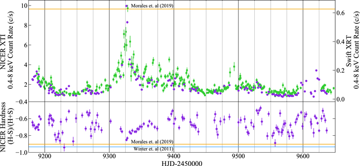
Figure 2. Top: NICER XTI (purple circles) and Swift XRT (green squares) light curves from 2020 November 28 to 2022 February 28. Uncertainties in the count rates are shown with thin bars for both sources. The NICER uncertainties are often smaller than the data point. For many observations between Days 9350–9450 and 9490–9500, during which strong variability is observed with Swift, NICER experienced high optical or particle background interference, which prevents precise background modeling. This results in filtered spectra with exposures <400 s and estimated background rates of >1 counts s−1, prompting their exclusion from the data set. For reference, estimated historical 0.4–8 keV NICER count rates are calculated from the unobscured power-law models from Winter et al. (2011; 18.74 counts s−1) and Morales et al. (2019; orange line, 9.64 counts s−1). These are calculated from the spectral models using the NICER response in Section 2. Bottom: NICER hardness ratio from 0.4 to 8 keV, demonstrating variability in spectral shape. The H band covers 3–8 keV, and the S band covers 0.4–3 keV. Estimated 0.4–8 keV NICER hardness ratios are shown for the aforementioned models from Winter et al. (2011; blue, hardness = −0.93) and Morales et al. (2019; orange, hardness = −0.91).
Download figure:
Standard image High-resolution imageTable 2. NICER Count Rate and Hardness
| Obs. Date | 0.4–8 keV | Hardness Ratio |
|---|---|---|
| (HJD −2,450,000) | Count Rate | H = 3–8 keV |
| (counts s−1) | S = 0.4–3 keV | |
| 9181.02 | 2.52 ± 0.06 | −0.64 ± 0.03 |
| 9181.67 | 2.46 ± 0.06 | −0.68 ± 0.03 |
| 9183.53 | 2.79 ± 0.06 | −0.68 ± 0.02 |
| 9185.53 | 2.88 ± 0.06 | −0.72 ± 0.02 |
| 9187.54 | 3.31 ± 0.05 | −0.70 ± 0.02 |
| ⋯ | ⋯ | ⋯ |
Only a portion of this table is shown here to demonstrate its form and content. A machine-readable version of the full table is available.
Download table as: DataTypeset image
3. Spectral Analysis
3.1. Spectral Model
Individual NICER observations are fit in XSPEC v12.12.0a (Arnaud 1996), starting with the best-fit model from the 2020 December 18 XMM observation introduced in Paper I. The model includes Galactic absorption (tbabs; Wilms et al. 2000) and a partially covering ionized obscurer (zxipcf; Reeves et al. 2008). The obscurer is defined in terms of its ionization parameter:

where L is the luminosity of the ionizing source in erg s−1 from 1 to 1000 ryd (13.6 eV–13.6 keV), n is the gas density of the ionized obscurer in cm−3, and R is the distance from the obscurer to the source in cm (Tarter et al. 1969). The AGN source spectrum is described by a power-law continuum, a soft excess produced by relativistically broadened reflection off of the inner accretion disk (relxillD), and an unobscured reflection component from distant, cold gas (xillverD; García & Kallman 2010). Contributions below 2 keV from two distant regions of photoionized emission, first discovered in the XMM-Newton/RGS spectra presented in Paper I, are modeled using pion_xs (Parker et al. 2019).
Following the methodology of Paper I, we also test an alternative scenario in which the soft excess is allowed to vary independently from the strength of the power-law continuum. Here the soft excess is described by a phenomenological blackbody model with the same obscuration as the power law. Unlike the models of the XMM-NuSTAR data in Paper I, we found that the models of the NICER data had degeneracies between the properties of the soft excess and the power-law components because there are fewer counts, particularly at the higher energies needed to constrain well the slope of the power-law component. In observations below 3 counts s−1, the model is completely insensitive to the presence of a soft excess, with the shape of the spectrum instead described solely by the properties of the power law and obscurer.
As an additional test, we fit the spectrum with a single obscured power law. While the trends in the column density of the obscurer are consistent with our final model, the absolute values tend to be modestly higher (the median increase is 17%). However, this model is unreliable, as the photon index is strongly degenerate with the column density of the obscurer. Typical values are Γ = 2.3 when the obscuration is low, as the model attempts to account for the soft excess, and Γ = 1.7 when the obscuration is high, since the continuum cannot be constrained below 3 keV.
This uncertainty in the shape of the soft emission forced us to fix the shapes of the soft excess and the power law in our standard analysis. In particular, we fix the power-law index to the XMM-NuSTAR model value of Γ = 1.9 based on Paper I, which includes a reflection-based soft excess tied to the power-law continuum. Changes in the strength of the power law are fit by the variable normalization of relxillD. Fixing the shape of the power law and soft excess for this analysis likely leads to an overestimate of the changes in the obscurer, although trends in the time evolution of the obscurer’s column density NH are little affected by this choice. Allowing the power-law index to vary leads to a difference in NH of at most 10% between the cases, which is less than the uncertainty in column density. The flux of the unobscured continuum is the parameter most significantly affected by the fixed power-law index.
The final XSPEC model is tbabs*(zxipcf*relxillD + xillverD + pion_xs + pion_xs), with four free model parameters: the normalization of the power-law continuum (relxillD), the hydrogen column density, the ionization parameter ξ, and the covering fraction of the obscurer (zxipcf). The allowed parameter ranges are listed in Table 1. Because the fluxes from distant emission regions in either the torus or X-ray BLRs (xillverD and pion_xs) are not anticipated to change significantly on the timescales of this campaign, the spectral parameters corresponding to these components are fixed at their Paper I values. All other parameters are also fixed to their respective Paper I values.
The model is first fit to each spectrum using a least-squares fit algorithm. This provides the initial conditions including covariances for a Markov Chain Monte Carlo analysis using an affine-invariant sampling algorithm (Goodman & Weare 2010). The chain has a total length of 100,000 steps across 100 walkers, with an initial burn in period of 20,000 steps. The median value and 68% confidence interval are calculated for each free parameter and reported in Figure 3 and Table 3.
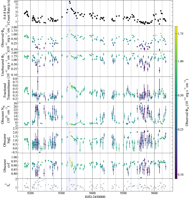
Figure 3. Variability of the obscurer and X-ray source in Mrk 817 from panel 1 (top) to panel 8 (bottom). The NICER light curve from in Figure 2 is shown in panel 1. The total observed flux of the inner X-ray source (described by relxillD only), including obscuration (ΦO ), is shown in panel 2, and the model-inferred intrinsic, unobscured flux (ΦU ) of the inner X-ray source is shown in panel 3. Panels 4–7 show the fractional transmittance (Equation (2)), hydrogen column density, ionization parameter, and covering fraction of the ionized obscurer, respectively. Panel 8 shows the reduced χ2 of the final maximum likelihood fit performed on each observation, as described in Section 3.1. The flare discussed in Sections 4.1 and 4.3 is highlighted in blue. In panels 2–6 the points are color-coded by ΦO following the color scale on the right.
Download figure:
Standard image High-resolution imageTable 3. Spectral Analysis Results: Observation Date and Spectral Parameters Fit Using the Methods in Section 3.1
| Obs. Date | 0.4–8 keV | 0.4–8 keV | Fractional | Obscurer NH | Obscurer | Obscurer | Best-fit |
|---|---|---|---|---|---|---|---|
| (HJD −2,450,000) |

|

| Transmittance | (1022 cm−2) |

| cvf |

|
| (erg s−1 cm−2 ) | (erg s−1 cm−2 ) | ||||||
| 9181.02 |

|

|

|

|

|

| 1.22 |
| 9181.67 |

|

|

|

|

|

| 1.21 |
| 9183.53 |

|

|

|

|

|

| 0.98 |
| 9185.53 |

|

|

|

|

|

| 1.05 |
| 9187.54 |

|

|

|

|

|

| 1.48 |
| ⋯ | ⋯ | ⋯ | ⋯ | ⋯ | ⋯ | ⋯ | ⋯ |
Note. Reported uncertainties correspond to the 68% confidence interval for each parameter. The first five observations are shown, with the full table published in machine-readable format.
Only a portion of this table is shown here to demonstrate its form and content. A machine-readable version of the full table is available.
Download table as: DataTypeset image
Flux values for individual model components are calculated using cflux in XSPEC over the 0.4–8 keV energy range.
3.2. Fractional Transmittance and Unobscured Flux
To quantify the effect of the obscurer on the observed flux, we define the obscurer’s fractional transmittance as

The observed flux (ΦO ) is the total flux from both the power-law continuum and the relativistically broadened reflection, after transmission through the partially covering obscurer (cflux*zxipcf*relxillD). The unobscured flux (ΦU ) is estimated by excluding the obscurer from the flux calculation (cflux*relxillD), thus providing the total flux of the “bare” continuum and broadened reflection (panels 2–4 of Figure 3). Contributions from distant emission are excluded from ΦO and ΦU .
3.3. Observed Variability
Comparison of individual NICER spectra demonstrates that observed variability is likely driven by two factors. Changes in the spectral shape of the source, particularly at energies below 3 keV, are interpreted to be caused by the variable transmittance of the obscurer (Figure 4, left panel), while broadband shifts in the flux are caused by changes in the unobscured flux of the X-ray continuum (Figure 4, right panel). This is illustrated by the changes in the hardness ratio of the source (Figure 2). Because changes in transmission alter the spectral shape while changes in the unobscured flux do not, the two likely sources of variability can be distinguished using the model framework introduced in Section 3.1.
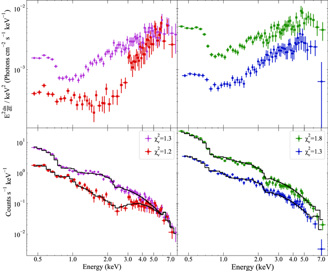
Figure 4. Top: photon count spectrum multiplied by E2 during four NICER observations, chosen to demonstrate how our models can distinguish a change in obscuration from a change in intrinsic flux. Bottom: photon count spectra for the same observations, with the best-fit models shown in black. Left: two observations that appear to demonstrate a change in obscuration. Observations taken on Day 9333 (purple circles) and Day 9267 (red squares) have a similar power-law continuum strength, as indicated by comparable count rate and spectral shape at E > 5 keV. Within our adopted model framework, we interpret this change as a difference in obscurer transparency leading to a change in spectral shape and brightness at soft energies. The obscurer’s fractional transmittance (Equation (2)) is  on Day 9333 and
  on Day 9267. Right: two observations that appear to demonstrate a change in intrinsic flux. The obscurer is in a similar state for both spectra, with NH = 3.6 × 1022 cm−2 on Day 3926 (green squares) and NH = 3.1 × 1022 cm−2 on Day 9341 (blue circles). The fractional transmittance values are
  and
and  and the log (ΦU
) values are
and the log (ΦU
) values are  erg s−1 cm−2 and
  erg s−1 cm−2, respectively.
Download figure:
Standard image High-resolution imageAn alternative scenario with a fixed obscurer, in which the change in spectral shape is driven solely by the power-law continuum, does not fit the data well. For example, compare the two spectra shown on the left in Figure 4. When the spectrum on Day 9333 is fit with fixed obscurer parameters equal to the values measured on Day 9267 (NH = 10.5 × 1022 cm−2,  , cvf = 0.94), the best fit has
  . This is much worse than the best-fit model for the same observation in the case of a variable obscurer, for which
  , NH = 3.0 × 1022 cm−2,
  , and cvf = 0.93. Such differences are typical of the other epochs, demonstrating that changes in the strength of the power law alone cannot produce the observed spectral variability.
To determine which characteristics of the obscurer are responsible for the variability, we first tested models in which only one of the three parameters, the hydrogen column density (NH), the ionization parameter ( ), or the covering fraction (cvf), is allowed to vary, while the others are fixed to the best-fit values from Paper I (NH = 6.95 × 1022 cm−2,
  , cvf = 0.93). If we define a fit with
  as acceptable, the NH-only model cannot fit 27% of the total observations, including those surrounding the observed peak on Day 9326. Similarly, a cvf-only model fails to fit 31% of the total observations. The better fits are generally for epochs with low count rates (<4 counts s−1). The
  -only model fails for 26% of the observations, most of which are below ∼2 counts s−1.
We next allow pairs of parameters to vary, with the third one fixed at its Paper I model value. Freezing  prevents a successful fit for 12% of observations, including those surrounding Day 9326, so the NH+cvf model is rejected. Both
  +cvf and
  +NH are able to explain the observed behavior near Day 9326, but the models fail for 12% and 6% of the observations, respectively, the majority of which are below ∼2 counts s−1.
The free NH+ +cvf model can describe the changes in the spectral shape across the full range of observed count rates, with only 1% of observations above the
  threshold. This motivates the decision to leave all three parameters free in the final models (panels 5–7 of Figure 3).
3.4. Correlation Analysis
We use the interpolated cross-correlation function (ICCF) to test for relationships between the X-ray and Swift UVW2 continua emission. Only with NICER can the unobscured X-ray continuum be estimated at the cadence required for this test. The ICCF, derived from the cross-correlation function (Peterson et al. 1998), allows for correlation tests between two light curves with uneven sampling. A linear interpolation of one light curve is tested for correlation with the comparison light curve at a range of time offsets, or “lags.” We use the ICCF program PyCCF (Sun et al. 2018) to test for a correlation between the Swift UVW2 flux curve (to be presented in Paper IV) and both the unobscured and obscured NICER X-ray continuum flux curves spanning Days 9181–9597 over a lag range from −15 to 15 days in steps of 0.01 days (Figure 5). The maximum correlation coefficient is R = 0.274 at 12.3 days between UVW2 and the observed X-ray flux and R = 0.275 at 0.7 days between UVW2 and unobscured X-ray flux (Figure 5).
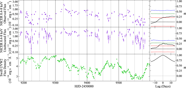
Figure 5. Swift UVW2 continuum light curve (green squares, bottom, Paper IV) with NICER observed flux (purple squares, top) and NICER unobscured flux (purple circles, middle) reproduced from Figure 3. CCFs with respect to the UVW2 reference band are shown to the right of each curve in black, with dashed curves representing the 68% (red), 95% (green), and 99.7% (blue) confidence intervals. No significant correlation above 95% confidence is measured.
Download figure:
Standard image High-resolution imageTo evaluate the significance of these lag measurements, the 68%, 95%, and 99.7% confidence limits for each ICCF are estimated using 10,000 simulated light curves. The power spectra are modeled as a damped random walk by fitting the measured light curves in Figure 3 using JAVELIN (Zu et al. 2011) to determine the parameters σ and τ (Kelly et al. 2009). The parameters are σ = 3.01 and τ = 9.18 days (observed NICER), σ = 6.26 and τ = 3.21 days (unobscured NICER), and σ = 6.61 and τ = 6.03 days (Swift UVW2). Light curves are simulated using these parameters and the method of Timmer & König (1995) and then sampled to match the real Swift and NICER observation dates. Gaussian noise is added using the observed uncertainty. The ICCF is measured for each set of simulated light curves, producing 10,000 R values at each lag from which confidence intervals are calculated. No correlation between either X-ray curve and the UVW2 curve is measured above 95% confidence.
4. Results
4.1. Variable Obscuration due to Column Density
Based on our estimates of the parameters of the obscurer (NH,  , and cvf), the hydrogen column density NH has the strongest impact on the fractional transmittance T of the gas during this campaign (the Pearson correlation R values between each parameter and T are −0.56, 0.33, and −0.20, respectively). This is best observed during extended periods of low transmittance (T < 0.4) when the obscurer has a high column density (NH > 1023 cm−2).
Our NICER observations began when the column density was low (NH < 1023 cm−2). NH increases from  to
to  between Days 9181 and 9213, corresponding to a drop in transmittance from
  to
to  . The first observed high column period state begins on Day 9215 and lasts for 87 days, with a maximum
 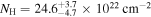 on Day 9221 and a minimum
  on Day 9257. While the obscurer is in the low-T state, changes in its covering fraction and ionization have little impact on its fractional transmittance (Figure 3, Table 3).
Subsequent high column density states are observed between Days 9436–9468 and Days 9544–9590, with similarly low transmittances. Also notable are the more rapidly occurring changes in NH from Day 9612 onward. This behavior amplifies the variability in the unobscured continuum, creating the minor flares observed during the last months of the campaign.
4.2. Covering Fraction of the Obscurer
The covering fraction cvf is the fraction of the continuum flux affected by the obscurer. A low covering fraction (cvf < 1) produces a steeper, power-law-shaped spectrum, indicating that photons are “leaking” through the obscurer. The median cvf = 0.92, and 90% of cvf values are between 0.83 and 0.96.
Unlike NH, the covering fraction is uncorrelated with the fractional transmittance of the source, indicating that the obscurer’s column density does not affect the fraction of photons that interact with it. Transmittance is driven by the strength of the absorption features, which increase while the obscurer is in a high column density state, rather than changes in the fraction of photons that interact with the obscurer. The implications of the stable covering factor on the geometry of the obscurer are discussed in Section 5.
4.3. Photoionization of the Obscuring Gas
Between Days 9317 and 9347, our models suggest that the obscurer has a low column density, with NH ≈ 3 × 1022 cm−2 and an initial  . The gas is ionized further during the X-ray flare between Days 9317 and 9326, as evidenced by an increase in ξ by almost an order of magnitude. The unobscured flux also increases by a factor of ∼2, corresponding to a change in observed flux by a factor of ∼3, before returning to its initial brightness on Day 9335. During this flare, the gas reaches a maximum
  on Day 9327, a day after the peaks in the observed and unobscured flux (seen in Figure 3). By Day 9347, the ionization of the gas falls to
  . Due to the combined reduction in NH and the increased transparency from photoionization, the transmittance of the obscurer increases from
  on Day 9273 to
  on Day 9326. The relationship between the unobscured X-ray flux and
  supports a scenario where the obscuring medium is ionized through photoionization from the central source.
A smaller local peak in the ionization parameter is seen 5 days after the bright peak on Day 9620, reaching a local maximum of  5 days after the flare (also visible in Figure 3). Both flares are observed while the obscurer has a low column density, enabling tight constraints on the state of the gas and the unobscured source. Due to the low count rates, measurements of the ionization parameter have much greater uncertainties when the obscurer has the highest column density, for example, between Days 9257 and 9289.
4.4. Connection to the UV Obscurer
As discussed in Paper I, the presence of a UV obscurer is indicated by the presence of broad absorption troughs in the COS UV continuum. Variability in the absorption strength of the X-ray obscurer, indicated by changes in NH, is closely tied to changes in the equivalent width of the broad UV absorption troughs throughout the campaign (Figure 6). We chose Si IV to illustrate the changes in the broad UV absorption strength since it is a resolved doublet that permits the most accurate assessment of optical depth and covering fraction. Of all the broad lines, it is the most optically thin, and it displays the greatest range in apparent optical depth.
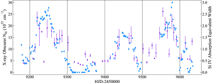
Figure 6. Time evolution of X-ray (left axis, purple circles) and UV (right axis, blue squares) continuum obscuration, characterized by the NH of the ionized absorber in NICER model and the equivalent width of the broad Si IV absorption trough in the COS spectra. The NICER data are binned in intervals of 5 days for clarity. The COS data are preliminary, processed using the methods in Paper I. Three distinct periods of heavy obscuration are observed concurrently in both energy ranges, suggesting that the observed emission from the X-ray corona and that from the the inner accretion disk are affected by the same obscuration along our line of sight.
Download figure:
Standard image High-resolution image5. Discussion
In Paper I we attributed the unprecedented low X-ray flux state of Mrk 817 to changes in the hydrogen column density of an ionized obscurer based on the average of five NICER epochs. We are now able to measure the spectral characteristics of both the X-ray source and the obscurer from individual observations. The parameter variation reveals much about the obscurer’s behavior, including rapid photoionization changes due to intrinsic source variability and multiple long periods of obscuration due to high column densities.
Changes by an order of magnitude in the column density of the obscurer occur on timescales of a few weeks. This is consistent with a scenario where a denser outflow develops, presumably from the accretion disk, and then flows into our line of sight, leading to stronger absorption of a more central X-ray source for a month or longer. This scenario may connect the variable density of the X-ray obscurer to the BLR holiday observed in Paper I if the denser outflow first passes between the UV continuum and the BLR.
In Mrk 817, the X-ray obscurer’s covering fraction is relatively constant and high with little correlation to the overall transmittance of the gas. While it is similar to the range measured in the warm X-ray obscurer of NGC 5548 (Mehdipour et al. 2016), their model uses a fixed column density of NH = 1.2 × 1022 cm−2, and small changes in the covering fraction appear to drive observed variability. This suggests that variations in NH may become the dominant cause of changes in obscuration when column density is high, since NH frequently exceeds 2 × 1023 cm−2 in Mrk 817.
The close relationship between the UV and X-ray absorption features indicates that both the X-ray and UV continuum sources are covered by the same obscurer along our line of sight, since they appear to be affected simultaneously by changes in the opacity of the obscurer. This is consistent with an AGN geometry that includes a compact X-ray corona located close to the central engine of the AGN and UV continuum emission from the inner accretion disk (see Figure 1 of Paper I).
The strength of the broad UV absorption features in Mrk 817 was linked to changes in the covering fraction of the UV obscurer in Paper I. Combined with the relatively stable covering fraction of the X-ray obscurer, this suggests that the UV absorbers may be the dense cores of weakly ionized material embedded in the X-ray obscuring outflow proposed in Krolik & Kriss (1995). If the X-ray obscurer is a combination of both diffuse regions and dense “knots,” which are also the UV absorbers, then the observed X-ray spectrum is an integration over all of those components along our line of sight.
As the knots become denser, and therefore less ionized, corresponding to a higher NH in the X-ray spectrum and stronger UV absorption (due to the lower ionization, the UV cross section of the knots increases), the photons that intercept the knots will become more highly absorbed and lead to a lower transmittance.
However, some photons avoid these knot regions, producing the observed cvf < 1. This does not require the obscurer to partially cover the X-ray source, which would be difficult to achieve if the X-ray source is compact and the obscurer is far away. The alternative is that the “leaked” flux is due to scattering. If the structure of the gas surrounding the knots does not change significantly while these knots evolve, then we would expect the same amount of unabsorbed light to leak through the diffuse region of the obscurer regardless of the current state of the dense knots. This produces a stable covering fraction in the X-ray spectrum uncorrelated with NH and the transmittance of the gas. As these cores pass our line of sight, the covering fraction of the UV obscuration should vary without requiring a change in the covering fraction of the more diffuse X-ray absorbing region. The limited filling factor of the knots required for this scenario may suggest clumping due to dynamical thermal instability, such as in Waters et al. (2022). Future analysis of the UV absorption model is expected to produce a geometric description of the obscurer consistent with both the observed X-ray and UV properties (G. Kriss et al. 2023, in preparation).
No significant correlations between the Swift UVW2 continuum and either the observed or unobscured X-ray continuum flux are detected, consistent with other AGNs where a disconnect between variability in the X-ray and UV continuum is observed. This is a significant challenge to the current paradigm of AGN physics. For Mrk 817, we hypothesize that this is caused by additional variable obscuration affecting the path from the X-ray source to the UV-emitting inner accretion disk, which would result in a disk ionized by a different spectral energy distribution than the one we observe. Future analysis with NICER of a brighter obscured source, in which the reflected component of X-ray emission can be separated from the continuum with higher confidence, may be the key to addressing this.
6. Summary and Conclusions
Spectral modeling of the X-ray emission and obscurer in Mrk 817 using 138 individual ∼1 ks NICER observations taken at a 2-day cadence reveals the following:
- 1.Changes in the hydrogen column density (NH) of the obscurer drive changes in the absorption of the X-ray coronal emission. The rapid changes from a high to low column density state suggest the presence of a clumpy outflow, presumably originating from the accretion disk.
- 2.The relationship between the changes in the X-ray absorption due to NH of the X-ray obscurer measured with NICER and the equivalent width of UV absorption troughs measured with HST/COS is preserved throughout the campaign. This provides strong evidence that both the X-ray and UV continuum emission are affected by the same obscuring gas.
- 3.Mrk 817 approaches its historical brightness during a short X-ray-luminous flare that peaks on Day 9326. This flare ionizes the obscuring gas, with a peak ionization parameter of
 ∼ 2 a day after the maximum unobscured flux. This occurs while the obscurer is in a low column density state, leaving the unobscured continuum highly visible and thus heightening the observed strength of the flare.

This analysis of Mrk 817 demonstrates NICER’s unprecedented capability to track the time-dependent ionization response of an obscuring gas due to variability in its irradiating X-ray source. Additionally, the measurements of NH and covering fraction obtained during individual NICER observations provide valuable information for determining the outflow dynamics of AGN winds. Future work on this subject aims to use NICER observations of obscured AGNs to directly test both X-ray photoionization and disk wind launching models.
The AGN STORM 2 project began with the successful Cycle 28 HST proposal No. 16196 (Peterson et al. 2020). E.P. and E.M.C. gratefully acknowledge support for NICER data analysis of Mrk 817 through NASA grant 80NSSC21K1935 and Swift data analysis through NASA grant 80NSSC22K0089. Work investigating NICER background models was supported by NASA grant 80NSSC21K1413. Y.H. acknowledges support from grant GO-16196 provided by NASA through the Space Telescope Science Institute, which is operated by the Association of Universities for Research in Astronomy, Inc., under NASA contract NAS5-26555. Research at UC Irvine is supported by NSF grant AST-1907290. H.L. acknowledges a Daphne Jackson Fellowship sponsored by the Science and Technology Facilities Council (STFC), UK. D.I., A.B.K, and L.Č.P. acknowledge funding provided by the University of Belgrade−Faculty of Mathematics (the contract 451-03-68/2022-14/200104), Astronomical Observatory Belgrade (the contract 451-03-68/2022-14/ 200002), through the grants by the Ministry of Education, Science, and Technological Development of the Republic of Serbia. D.I. acknowledges the support of the Alexander von Humboldt Foundation. A.B.K. and L.Č.P acknowledge the support by the Chinese Academy of Sciences President’s International Fellowship Initiative (PIFI) for visiting scientist. M.C.B. gratefully acknowledges support from the NSF through grant AST-2009230. A.Z. is supported by NASA under award No. 80GSFC21M0002. A.V.F. is grateful for financial assistance from the Christopher R. Redlich Fund and numerous individual donors. M.V. gratefully acknowledges financial support from the Independent Research Fund Denmark via grant No. DFF 8021-00130.
This research has made use of data obtained through the High Energy Astrophysics Science Archive Research Center Online Service, provided by the NASA/Goddard Space Flight Center. This work has made of NICER observations acquired by a Target of Opportunity request (Target ID: 320186) and GO proposal 4128, and we thank the NICER operations team for their work in acquiring this data set.
We are grateful to the members of the NICER instrumentation and science teams for their valuable suggestions and feedback during the background selection and data reduction stages of this analysis. In particular, we thank Ronald Remillard, Michael Loewenstein, Craig Markwardt, and James Steiner for their generous input.
Facilities: NICER - , Swift - , Hubble COS. -
Software: Astropy (The Astropy Collaboration et al 2013), Matplotlib (Hunter 2007), HEASOFT (http://heasarc.gsfc.nasa.gov/ftools), ftgrouppha (Kaastra & Bleeker 2016), NICER Space Weather Estimator (https://heasarc.gsfc.nasa.gov/docs/nicer/tools/nicer_bkg_est_tools.html), NICER 3C50 Estimator (Remillard et al. 2022), NICER Machine Learning Estimator (https://github.com/zoghbi-a/nicer-background), Swift XRT Light Curve Generator (Evans et al. 2007, 2009), XSPEC (Arnaud 1996), tbabs (Wilms et al. 2000), relxillD (García et al. 2016), xillverD (García & Kallman 2010), pion_xs (Parker et al. 2019), PyCCF (Peterson et al. 1998; Sun et al. 2018), JAVELIN (Zu et al. 2011), SciPy (Virtanen et al. 2020).
: Appendix
As discussed in Section 2, background subtraction in NICER is complex because it is not an imaging telescope. Because we have contemporaneous Swift observations during almost all of the NICER observations, we can use Swift to test the NICER background models by evaluating how well each background-corrected NICER observation predicts the near-simultaneous Swift observations (or vice versa).
We first process each NICER observation using the three available background estimators as detailed in Section 2. We use observations taken between Day 9181 and Day 9599, corresponding to Swift’s first uninterrupted period of observation, and only observations with exposures >400 s. This selection criterion results in 162 observations with the 3C50 estimator, 197 with the Machine Learning estimator, and 192 with the Space Weather estimator (Table 4). The reduced number of 3C50 spectra is due to the aggressive filtering process native to this estimator. Source count rates are equal to the total count rate of the observation minus the estimated background. The stricter filtering for the 3C50 background results in shorter good time intervals with different total rates.
Table 4. NICER Source and Background Count Rate for Each Estimator during the Period of Continuous Swift Monitoring
| Obs. Date | 3C50 | 3C50 | Machine Learning | Machine Learning | Space Weather | Space Weather |
|---|---|---|---|---|---|---|
| (HJD −2,450,000) | 0.4–8 keV | 0.4–8 keV | 0.4–8 keV | 0.4–8 keV | 0.4–8 keV | 0.4–8 keV |
| Source Rate | Background Rate | Source Rate | Background Rate | Source Rate | Background Rate | |
| (counts s−1) | (counts s−1) | (counts s−1) | (counts s−1) | (counts s−1) | (counts s−1) | |
| 9189.21 | 2.20 ± 0.07 | 0.36 | 2.25 ± 0.07 | 0.35 | 1.98 ± 0.07 | 0.63 |
| 9190.32 | 3.01 ± 0.03 | 0.56 | 3.22 ± 0.03 | 0.44 | 2.49 ± 0.03 | 1.17 |
| 9190.71 | 2.35 ± 0.03 | 0.38 | 2.46 ± 0.03 | 0.38 | 2.15 ± 0.03 | 0.68 |
| 9191.61 | 1.98 ± 0.03 | 0.50 | 2.10 ± 0.03 | 0.49 | 1.94 ± 0.03 | 0.65 |
| 9193.74 | 1.79 ± 0.03 | 0.38 | 1.88 ± 0.03 | 0.38 | 1.59 ± 0.03 | 0.68 |
| ⋯ | ⋯ | ⋯ | ⋯ | ⋯ | ⋯ | ⋯ |
Note. The first five observations are listed, with the full table published in machine-readable format. Observations where an estimator failed or filtering reduced the exposure below 400 s are listed as “...” in the appropriate column.
Only a portion of this table is shown here to demonstrate its form and content. A machine-readable version of the full table is available.
Download table as: DataTypeset image
Taking advantage of the high sampling rate of the coordinated Swift observations, we linearly interpolate the 0.4−8 keV Swift light curve to each NICER epoch, which provides a baseline for comparison with each NICER estimator’s background-subtracted light curve (Figure 7). Because the Machine Learning and Space Weather estimators lack an intrinsic outlier filtering process, their background-subtracted count rates for several observations agree with neither the interpolated Swift count rate nor the other estimators. These observations are circled in Figures 7–9 and are excluded from the correlation analyses.
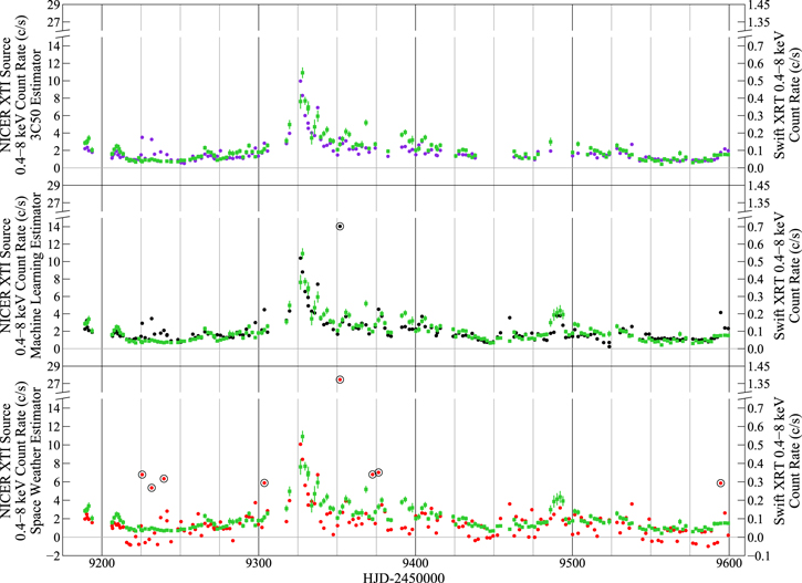
Figure 7. Background-subtracted NICER XTI light curves from the 3C50 (top, purple circles), Machine Learning (middle, black circles), and Space Weather estimators (bottom, red circles). The linearly interpolated Swift XRT count rates (green squares) are shown for comparison. Encircled observations are marked as outliers owing to their large deviation from interpolated Swift count rates.
Download figure:
Standard image High-resolution imageFigure 8 shows the background count rate light curves from all three estimators. The range of background rates is largest in the Machine Learning estimator owing to its attempt to continuously measure the background during each second of observation, with no rejection of background flares. Background rates from the 3C50 estimator are lower overall because it screens flares by dividing the spectrum into 30 s time intervals and excludes those with high residuals outside of NICER’s source sensitivity range (the 0.2–0.3 keV and 13–15 keV bands; see Remillard et al. 2022). The Space Weather estimator produces background count rates in either a high or low mode, centered at 2 counts s−1 and below 1 counts s−1, with negative source count rates for 24 observations. This indicates a lack of precision and suggests that the Space Weather estimator is unsuitable for analysis of faint sources such as Mrk 817. It also uses only the ISS location and space weather parameters with no internal estimates or filters for background flares.
Figure 8. NICER XTI background count rate light curves from the C50 (top, purple), Machine Learning (middle, black), and Space Weather estimators (bottom, red). The outliers in Figure 7 are encircled in black.
Download figure:
Standard image High-resolution imageTo quantify the consistency between Swift and NICER for each estimator, we calculate the Pearson correlation coefficient R between the interpolated Swift prediction and the three NICER background-subtracted count rates. We restrict our analysis to observations with background rates <1 counts s−1, calculated without failure by all three estimators, for a total of 64 observations. We determine the best-fit scaling factors between the two instruments, taking into account the uncertainties in both light curves using the SciPy linear orthogonal distance regression (ODR; Boggs & Rodgers 1990) with a variable slope m and intercept b (Figure 9). Here the slope of the ODR line (m) is the scaling factor, with an exact match to the Swift count rates corresponding to m = 1. Systematic over- or underprediction of Swift count rates is indicated by a nonzero intercept b.
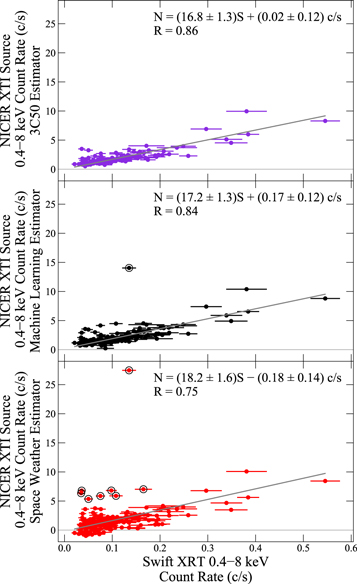
Figure 9. NICER source count rates produced by the 3C50 (top, purple), Machine Learning (middle, black), and Space Weather estimators (bottom, red), compared to the interpolated Swift count rate predictions for the date of each NICER observation. The outliers in Figure 7 are encircled in black. The best-fit ODR line (gray) excludes observations with background rates > 1 counts s−1 or where one or more estimators fail or are filtered out.
Download figure:
Standard image High-resolution imageThe scaling and correlation are 3C50 (R = 0.86, m = 16.8 ±1.3, and b = 0.02 ± 0.12), Machine Learning (R = 0.84, m = 17.2 ± 1.3, and b = 0.17 ± 0.12 counts s−1), and Space Weather (R = 0.75, m = 18.2 ± 1.6, b = − 0.18 ± 0.14 counts s−1). The higher scaling factors for Machine Learning and Space Weather may indicate that 3C50 background rates are overpredicted. However, the outliers from the other two estimators suggest a more likely scenario where background flares filtered out by 3C50 are underestimated by Space Weather and Machine Learning, thus contaminating their source count rates.
We also measured the correlations between the source and background rates for each estimator, with R = 0 expected if the modeled background is accurate. This is confirmed for the 3C50 (R = 0.06) and Machine Learning (R = 0.07) estimators. A negative correlation is found for the Space Weather estimator (R = −0.46), indicating that the background is being systematically overestimated in the high background mode and/or systematically underestimated in the low background mode. This supports the hypothesis that the Space Weather estimator is unsuitable for analysis of faint sources.
The source and background rates of the 3C50 and Machine Learning estimators are also compared directly, using observations that meet the 3C50 filtering criteria. The source rates are strongly correlated (R = 0.97), although the count rates of only 7% of the observations are consistent given their uncertainties. Source rates for Machine Learning are typically higher ( counts s−1 and
  counts s−1, where
  is the mean source count rate after outlier exclusion). This demonstrates a systematic offset in the count rate estimates due to the different modeling and outlier rejection processes. The correlation between background rates is weaker (R = 0.77) owing to the background filtering process of 3C50. A weak negative correlation is found when comparing the 3C50 background rate to the difference in the source (R = −0.19) and background rates (R = −0.22) between the two estimators, indicating that they do not estimate or filter observations consistently with one another when background activity is high. We find a mean systematic uncertainty of
  between the two estimators for the 0.4–8 keV range, where σ = ∣r3C50 − rML∣/r3C50 and r is the source count rate.
Due to the robust 3C50 filtering process, we analyze the spectra produced by the 3C50 model. After excluding any observations with background rates >1 counts s−1, we have a total of 153 observations.
Footnotes
- 43
All dates are reported in terms of Heliocentric Julian Date (HJD)-2450000.
- 44