Abstract
Monitoring of vibrational eigenmodes of an elastic body excited by gravitational waves was one of the first concepts proposed for the detection of gravitational waves. At laboratory scale, these experiments became known as resonant bar detectors first developed by Joseph Weber in the 1960s. Due to the dimensions of these bars, the targeted signal frequencies were in the kHz range. Weber also pointed out that monitoring of vibrations of Earth or the Moon could reveal gravitational waves in the mHz band. His Lunar Surface Gravimeter experiment deployed on the Moon by the Apollo 17 crew had a technical failure, which greatly reduced the science scope of the experiment. In this article, we revisit the idea and propose a Lunar Gravitational-Wave Antenna (LGWA). We find that LGWA could become an important partner observatory for joint observations with the space-borne, laser-interferometric detector LISA and at the same time contribute an independent science case due to LGWA’s unique features. Technical challenges need to be overcome for the deployment of the experiment, and development of inertial vibration sensor technology lays out a future path for this exciting detector concept.
Original content from this work may be used under the terms of the Creative Commons Attribution 4.0 licence. Any further distribution of this work must maintain attribution to the author(s) and the title of the work, journal citation and DOI.
1. Introduction
With the first detection of gravitational waves (GWs) from a merging binary black hole (BBH) finally achieved in 2015 (Abbott et al. 2016a), the field of GW astronomy is still in its infancy. It has already revolutionized multimessenger astrophysics (Abbott et al. 2017a, 2017b), has led to important constraints on stellar evolution models (Abbott et al. 2019a, 2020c), and has put strong constraints on alternative theories of gravity (Baker et al. 2017), but its main impact on cosmology (Abbott et al. 2009, 2017c) and fundamental physics (Arvanitaki & Dubovsky 2011; Yunes et al. 2016; Abbott et al. 2018a; Cardoso et al. 2019; Abbott et al. 2019b) is yet to come.
We should expect that the vastness of the yet-unfulfilled GW science case will manifest itself in a diversification of the detector concepts to cover the entire frequency band from the slowest possible spacetime oscillations observable in our Hubble volume (of order 10−18 Hz) to the kHz region, where we expect the highest-frequency signals produced by astrophysical sources. Detector concepts include, from low to high observed frequencies, the cosmic microwave background B-mode polarization experiments (Ade et al. 2014), the pulsar timing arrays (Hobbs et al. 2010), monitoring of stellar oscillations (Siegel & Roth 2011; Lopes 2017), monitoring of planetary oscillations (Dyson 1969; Ben-Menahem 1983), space-based laser-interferometric detectors (Phinney et al. 2003; Sato et al. 2009; Luo et al. 2016; Amaro-Seoane et al. 2017), and ground-based ones (Harms et al. 2013; Canuel et al. 2020; Paik et al. 2020; The LIGO Scientific Collaboration 2015; Acernese et al. 2015; Souradeep 2016; Akutsu et al. 2019). In addition to the observation band, detectors can also be distinguished by their internal configuration, which has an impact on the information that can be extracted from GW signals (Bianchi et al. 1996; Sathyaprakash et al. 2012; Paik et al. 2016), most notably the ability to measure the polarization of a GW and to estimate its propagation direction.
It was Pirani who first studied in great detail the observable effects of GWs (Pirani 1956), and Weber conceived the first detector concept, i.e., the resonant bar detector (Weber 1960). Weber’s efforts were essential to start the field of experimental GW detection, which first developed into a global network of resonant bar detectors (Amaldi et al. 1989; Allen et al. 2000). It was also understood that Earth itself has an elastic response to GWs. A first analysis leading to an upper limit for GW energy passing through Earth was obtained in 1961 by Forward et al. (1961), and a possible detection was claimed 10 yr later by Tuman (1971). The Lunar Surface Gravimeter experiment, brought on the Moon by the Apollo 17 mission in 1972, had the main scientific target of detecting GWs, but a technical failure rendered the data useless (Giganti et al. 1977; Bates et al. 1979). In 2008, the feasibility of a lunar GW detector based on Weber’s idea was again discussed in light of new technological developments (Paik & Venkateswara 2009).
Calculations of cross sections of elastic bodies to GWs were presented in some of the earliest publications on GW detection, but detailed calculations of the coherent GW response were not known until the end of the 1960s. Dyson calculated the response of a homogeneous, elastic half-space to GWs (Dyson 1969), and the formalism to calculate the response of a laterally homogeneous spherical body was developed by Ben-Menahem (1983). Spherical, laboratory-scale GW detectors were first proposed by Coccia et al. (1995), and their science potential was investigated especially with respect to testing theories of gravity (Bianchi et al. 1996).
Work published in a recent series of papers has demonstrated that scientifically interesting GW sensitivities can be achieved by monitoring seismic fields (Coughlin & Harms 2014a, 2014b, 2014c). The new analyses were based on state-of-the-art detection pipelines developed by the Virgo and LIGO communities and modified to be applied to a network of seismometers or gravimeters monitoring vibrations of Earth (Coughlin & Harms 2014a, 2014c) or the Moon (Coughlin & Harms 2014b). The Dyson half-space response was exploited in Coughlin & Harms (2014b, 2014c), which is a valid model at higher frequencies where individual normal modes cannot be resolved anymore, and the Ben-Menahem equations for normal-mode excitation were used in Coughlin & Harms (2014a). In terms of GW energy density, the new constraints were better by more than 10 orders of magnitude compared to previous limits obtained from high-precision laboratory experiments. The sensitivity limitations of these studies were a product of a trade-off between selecting the quietest data stretches to minimize seismic correlations and using as much data as possible to minimize statistical errors. This trade-off has an optimum when the seismic correlations match the statistical errors. For Moon data, relatively few data stretches had to be excluded from the reported GW analyses, and since the stationary noise is also significantly quieter on the Moon compared to Earth, which reduces the statistical errors, a much better GW sensitivity resulted with Moon data.
With the Lunar Gravitational-Wave Antenna (LGWA), we propose to deploy an array of high-end seismometers on the Moon to monitor normal modes of the Moon in the frequency band 1 mHz–1 Hz excited by GWs (Harms et al. 2020c). Several properties of the Moon make it an ideal candidate as a GW detector: (1) it is the closest body to Earth, (2) it is large, (3) it lacks an atmosphere and ocean, and (4) it has much lower seismic activity than Earth. Moonquakes and meteoroid impacts occur (several thousand were identified by the Apollo Lunar Surface Experiments Package (ALSEP); Nakamura et al. 1981; Lognonné & Mosser 1993), but the magnitudes of these events are all minor. Most important is that the ambient field, i.e., a stationary background to the moonquakes and impacts, is so quiet that it was not possible to observe it with ALSEP.
Using technology with high readiness level, the experiment could run within the next decade, i.e., together with the LISA mission (Amaro-Seoane et al. 2017) or the third-generation, ground-based detectors Einstein Telescope (ET; Punturo et al. 2010) and Cosmic Explorer (Reitze et al. 2019). Since its performance would improve with the development of new vibration sensing technology, it has the potential to become a lasting contribution to the future GW detector network. We also point out that large-scale, laser-interferometric GW detector concepts have been proposed for the Moon (Stebbins & Bender 1990; Jani & Loeb 2020; Katsanevas et al. 2020).
In Section 2, we describe in detail the important aspects of the detector concept presenting sensitivity requirements and compatibility with the current state of technology. The components of the LGWA concept are brought together in Section 3 to obtain sensitivity predictions for LGWA following several GW search methods. The LGWA science case, which includes the direct analysis of GW signals and of the corresponding electromagnetic counterparts detectable by Earth-based and satellite telescopes, is summarized in Section 5. The deployment and operation of the array poses certain practical challenges, which are outlined in Section 4.
2. Detector Concept
In order to assess the quality of a GW detector concept, it is useful to divide the detector into a readout system and a response body. We understand the response body as an abstract term, which can refer to a laser beam, suspended test masses, clocks, or an elastic body, which can all be affected by a passing GW. At this level, the description of the response can depend on the coordinate system used to describe the experiment. The readout system consists of the coupling dynamics to the response body and the translation of the GW signal into a human-readable form. The quality of a GW detector concept then hinges on three main criteria:
- 1.How strongly does the body respond to GWs?
- 2.How sensitive is the readout system to changes in the response body affected by GWs?
- 3.What is the level of environmental or intrinsic random excitation of the response body?
Response: In the case of LGWA, the response body is the Moon itself. The strength of the response is described by the following relation between GW strain amplitude h and seismometer displacement signal ξ:

where i is the imaginary unit and f is the signal frequency. The equation neglects any angular dependence of the response. The sum is over the vibrational quadrupole modes of order n of the Moon characterized by a mode frequency fn and a quality factor Qn . The parameter Ln describes an effective baseline, which can take a complicated form depending on how the amplitude of a mode varies inside the Moon as a function of the distance to its center. All three parameters depend strongly on the internal structure of the Moon (Ben-Menahem 1983). It should also be noted that displacements are produced in the vertical direction (by spheroidal modes) and in the horizontal (by both spheroidal and toroidal modes). The excitation of toroidal modes by GWs is strongly suppressed, i.e., toroidal modes cannot be excited at all by GWs in a homogeneous body (Bianchi et al. 1996). We neglect toroidal modes in the following.
Note that ξ is not (necessarily) the surface displacement induced by GWs, but the difference of surface displacement and direct seismometer test mass displacement caused by gravitational fluctuations. It was shown in Section 2.1.3 of Harms (2019) that this is the natural dynamical variable in models where gravitational strain produces elastic deformations instead of Newtonian gravity potentials. In these coordinates, the effective baseline Ln does not have to be positive, but it is always real-valued (Ben-Menahem 1983).
If the signal frequency f coincides with one of the lower-order normal-mode frequencies, which are expected to have Q-values of a few hundred at least, then the response can be approximated as

This result allows us to calculate order-of-magnitude estimates of displacement signals produced by GWs. With a strain amplitude of 10−21 as can be expected for loud galactic double white dwarfs (DWDs; Kupfer et al. 2018; Lamberts et al. 2019), a Q-value of 200, which can be expected for the lowest-order quadrupole modes, and an effective baseline of Ln = 0.6R (Coccia & Fafone 1996; Coughlin & Harms 2014b), where R = 1.7 × 10⁶ m is the radius of the Moon, one obtains displacement signals of order ξ ∼ 10−13 m. This response is similar in magnitude to the response in the LISA detector, where it is achieved with a much longer baseline (L = 2.5 × 10⁹ m), but over a broad band without any resonant amplification factor.
Another regime of interest is the high-frequency response (around 0.1 Hz), where it will be difficult to identify excitations of individual normal modes. It turns out that the effective baseline Ln drops very quickly with increasing order n (Coccia & Fafone 1996). This means that the response can be approximated by truncating the sum in Equation (1) such that all of the included modes have frequencies well below 0.1 Hz. The result for our fiducial response model is shown in red in Figure 1.
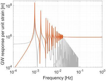
Figure 1. Simplified GW response model (red) used in this paper, with normal-mode sum truncated at n = 22. The response curve of a pessimistic response model is shown in gray for comparison. The models only include spheroidal quadrupole modes.
Download figure:
Standard image High-resolution imageIts truncated high-frequency response can be approximated as

where  at
at  . The Q-values do not play a role anymore, and the truncated sum over Ln
now defines the overall effective baseline. Since in general the baselines Ln
can also take negative values (Coughlin & Harms 2014a), which depends on the Moon’s internal structure, there is a partial cancellation of baselines in the sum, reducing the high-frequency GW response of the Moon. Intuitively speaking, the question is how the softness of the Moon evolves with increasing frequency. In the limit f → ∞, the GW response as measured by a seismometer must vanish since the Moon’s elastic forces cannot withstand the effective tidal force of a GW. The Dyson response model predicts a 1/f approach to this limit (Dyson 1969), but details of the geology, including the damping of modes, have an important influence on the GW response up to frequencies well above the LGWA band, which means that a simple dependence on frequency should not be expected. The response above 10 mHz shown in Figure 1 is an upper limit, since it assumes that all normal-mode excitations up to order n = 22 add constructively and the Moon partially withstands tidal forces even at higher frequencies. In comparison, an alternative model is shown in gray for the differential response between the inertial reference of the seismometer and the Moon’s surface. Here, the Moon becomes maximally soft to tidal fields at high frequencies, which reduces the differential motion and therefore the GW signal. The true response of the Moon depends strongly on geology, but we can expect it to be somewhere between the red and gray curves above 20 mHz.
. The Q-values do not play a role anymore, and the truncated sum over Ln
now defines the overall effective baseline. Since in general the baselines Ln
can also take negative values (Coughlin & Harms 2014a), which depends on the Moon’s internal structure, there is a partial cancellation of baselines in the sum, reducing the high-frequency GW response of the Moon. Intuitively speaking, the question is how the softness of the Moon evolves with increasing frequency. In the limit f → ∞, the GW response as measured by a seismometer must vanish since the Moon’s elastic forces cannot withstand the effective tidal force of a GW. The Dyson response model predicts a 1/f approach to this limit (Dyson 1969), but details of the geology, including the damping of modes, have an important influence on the GW response up to frequencies well above the LGWA band, which means that a simple dependence on frequency should not be expected. The response above 10 mHz shown in Figure 1 is an upper limit, since it assumes that all normal-mode excitations up to order n = 22 add constructively and the Moon partially withstands tidal forces even at higher frequencies. In comparison, an alternative model is shown in gray for the differential response between the inertial reference of the seismometer and the Moon’s surface. Here, the Moon becomes maximally soft to tidal fields at high frequencies, which reduces the differential motion and therefore the GW signal. The true response of the Moon depends strongly on geology, but we can expect it to be somewhere between the red and gray curves above 20 mHz.
Readout: The second criterion, the quality of the readout system, is defined by the seismometers used to monitor seismic fields. The most sophisticated seismic sensor deployed outside Earth is the SEIS experiment of the Mars Insight mission (Lognonné et al. 2019). It achieves an acceleration sensitivity of about  at mHz frequencies (Mimoun et al. 2017). There is significant margin, though, for sensitivity improvements. The SEIS noise budget contains atmospheric disturbances and noise from thermal processes (Mimoun et al. 2017). For this reason, it is expected that the SEIS technology on the Moon would immediately lead to a 10-fold better sensitivity. Another major improvement can be obtained by realizing that seismometers in LGWA do not need to monitor vertical displacement. This means that the stiffness of the mass suspensions can be further reduced (Winterflood 2002; Bertolini et al. 2006), leading to lower suspension resonance frequencies and improved response of the sensor to ground motion. In addition, substituting the capacitive readout of the test mass position by an optical readout promises a significant gain in low-frequency sensitivity (De Rosa et al. 2011; Berger et al. 2014). As another solution, one can consider magnetic levitation of a test mass (Paik & Venkateswara 2009). Operating such a system at cryogenic temperatures would be ideal and push the fundamental sensitivity limits of seismic sensing, but since the practical challenges of a cryogenic sensor on the Moon might be too severe, an optical readout of a suspended mass at ambient temperature could be used and achieve superior sensitivities.
Figure 2 shows an optomechanical and cryomagnetic seismometer concept for LGWA, together with the noise performance of the Mars Insight Very Broadband (VBB) sensors and of the LISA Pathfinder (LPF) mission (Armano et al. 2016; Anderson et al. 2018), which is the best acceleration sensitivity ever achieved at mHz frequencies. The Mars Insight model combines the position and velocity readouts of the suspended masses. Details of the two LGWA concepts can be found in Section 4.4.
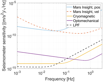
Figure 2. LGWA seismometer concepts (cryomagnetic and optomechanical) in comparison with the performance of Mars Insight VBB sensors (Mimoun et al. 2017) and with the acceleration sensitivity of the LISA Pathfinder mission (Anderson et al. 2018).
Download figure:
Standard image High-resolution imageIntrinsic noise: The last criterion concerns the intrinsic quietness of the Moon. The small tide signature and the absence of oceans set the background noise level well below the low-noise model for Earth, which was first defined by Peterson in 1993 (Peterson 1993). This enhances the capability of seismometers to detect natural events both endogenic (as moonquakes) and exogenic (as GWs). There are four different classes of natural seismic events on the Moon (in addition to artificial impact events):
- 1.deep moonquakes probably produced by tides;
- 2.shallow moonquakes a few tens of kilometers below the surface;
- 3.thermal quakes;
- 4.meteoroid impact.
About 12,500 such events were identified over the course of 9 yr and with up to four seismometers monitoring in parallel by ALSEP (Nakamura et al. 1981; Khan et al. 2013). Even though the number seems high, the annual rate of seismic energy release on the Moon is very small, 4–8 orders of magnitude smaller than on Earth (Khan et al. 2013). It is expected that the dominant noise background is produced by the impact of meteoroids, which have a relatively high flux for small masses (Grün et al. 2011) (only 1700 impacts were strong enough to be identified by ALSEP; Khan et al. 2013). The value of this background was estimated to be around  between 0.25 and 2 Hz (Lognonné & Mosser 1993), which lies about an order of magnitude above the readout noise of the cryomagnetic concept at these frequencies, falling under LGWA instrument noise below 10 mHz. Our new estimate based on normal-mode response provided in the Appendix places the meteoroid background below the targeted sensitivity over the entire observation band. Future work must reconcile the two approaches.
3. LGWA Sensitivity
The basic noise spectral density Sh (f) of LGWA in units of GW strain h is obtained by dividing the readout noise shown in Figure 2 by the GW response model in Equation (1). Here, we assume a Q-value of 300 for all quadrupole modes and use a simplified (homogeneous) model of the Moon. The square root of Sh (f) is shown in Figure 3, together with the noise target of the LISA detector (Amaro-Seoane et al. 2017).
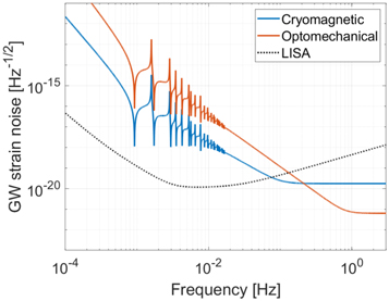
Figure 3. Predicted LGWA noise spectral density.
Download figure:
Standard image High-resolution imageInterestingly, LGWA has the potential to beat LISA sensitivity above 0.1 Hz, which might be interesting for observations of DWD mergers. Its noise consists of a series of narrowband features inherited from the normal-mode response. However, above 10 mHz, the response becomes broadband dominated by the above-resonance response of the low-order quadrupole normal modes.
In the initial proposal of LGWA (Harms et al. 2020c), a division of the mission into phase 1 and phase 2 was foreseen (see Section 4). Phase 1 included the deployment of an array of nearby seismometers, while phase 2 referred to the deployment of an additional seismometer on the opposite side of the Moon. Phase 2 is required for GW detections relying on correlation between seismometers as necessary for stochastic GW backgrounds (Coughlin & Harms 2014c). The main issue here is the background noise produced by the meteoroid impacts. Correlating data between two nearby instruments, one can reject contributions from readout noise, but one will likely observe a partial correlation of the meteoroid background noise, which would pose a strong sensitivity limitation to stochastic GW searches. Instead, a near antipodal location of the phase 2 sensor would have very small or negligible correlations from seismic sources, but the correlation of GW signals is still maximal.
A sensitivity with respect to the stochastic GW signal is typically expressed in units of an energy density relative to the critical energy density of the standard cosmological model (Allen 1996). For an optimally positioned (antipodal) pair of seismometers, one obtains the following sensitivity to measurements of the fractional energy density of GWs:

where H0 is the Hubble constant and Tobs is the total observation time. The factor fTobs represents the number of averages one can maximally do to estimate the cross-spectral density at frequency f between the two seismometers (Sharma & Harms 2020).
The resulting noise prediction for measurements of GW energy density is shown in Figure 4 with a total observation time of 3 yr.
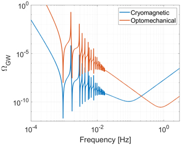
Figure 4. Predicted LGWA sensitivity to stochastic GW backgrounds.
Download figure:
Standard image High-resolution imageThe most sensitive searches of GWs could be carried out by matching the (still unknown) normal-mode frequencies of the Moon with catalogs of DWDs (Kupfer et al. 2018). These binaries emit GWs at known and slowly increasing frequencies, and their waveforms can be predicted. Alternatively, one could search over entire regions of the DWD parameter space to detect unknown DWD systems, which is the standard matched-filter search carried out for the current ground-based GW detectors. In either case, the minimal value of the GW amplitude that can be resolved is (Harms et al. 2013)

where σ is the signal-to-noise ratio threshold for a GW detection. The noise level of this measurement, i.e., the last equation with σ = 1, is shown in Figure 5 for a 5 yr observation time.
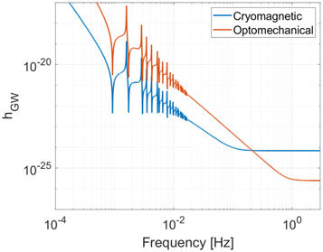
Figure 5. Predicted LGWA sensitivity to near-monotonic GW signals.
Download figure:
Standard image High-resolution image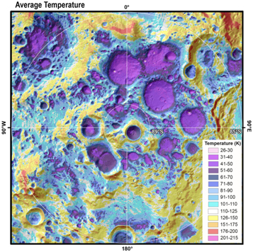
Download figure:
Standard image High-resolution image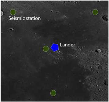
Figure 7. Configuration of the kilometer-scale LGWA array. Lander position is indicated for the case when all seismic stations are deployed from a single landing site. Separate landings are possible.
Download figure:
Standard image High-resolution imageIn order to be able to interpret this result as GW amplitude noise, one must assume that the frequency of the signal does not change significantly over periods of a few years as is the case for all mHz DWDs. Merger times of massive BBHs would be shorter, which means that within a year such a source could ring up normal modes in a temporal sequence from low to high frequencies. The analysis of LGWA data above 10 mHz can follow conventional methods with respect to all types of GW signals since the sensitivity loses its peaked features.
4. Implementation and Technologies
4.1. Lunar Surface Environment
Several environmental factors can be important for LGWA, including lunar dust (Grün et al. 2011), lunar surface temperature (Williams et al. 2017), cosmic rays and charges (Stubbs et al. 2006; Jordan et al. 2014), and the surface magnetic field (Lin et al. 1998).
The dust cloud surrounding the Moon can be important for the operation of sensitive equipment. Overheating of the Apollo 11 seismometer was attributed to dust deposition (O’Brien 2012; likely connected to the launch of the lunar module). It is certainly important to keep in mind for the instrument design that sensitive parts are not exposed to the environment.
Surface temperatures during lunar nights can fall close to 100 K and rise up to 400 K during lunar days (Williams et al. 2017). As will be explained in Section 4.4, of particular interest is the south pole of the Moon, with its permanently shadowed regions (PSRs), where temperatures well below 100 K can be found as shown in Figure 6 (Paige et al. 2010). These could be used as natural cryostats for a lunar seismometer.
Another potentially interesting but technologically challenging deployment location are lava tubes (Sauro et al. 2020; Theinat et al. 2020), where temperatures are expected to be more stable around the average ground temperature of 250 K (Horvath & Hayne 2018).
Radiation, for example, in the form of galactic cosmic rays, can damage electronics (Duzellier 2005). Radiation hardening is a common technique to make electronics more resistant against ionizing radiation. In addition, cosmic rays can lead to continuous charging of the lunar regolith, which can develop significant electric field strengths (Jordan et al. 2014).
Finally, seismic sensors as required for LGWA can be susceptible to fluctuations of the magnetic field (Ackerley 2015). Such fluctuations have not been characterized in detail on the lunar surface yet, but past measurements indicate that the magnetic field is about a factor of 1000 weaker than on Earth (Lin et al. 1998). Even if this factor extended to the magnetic fluctuations, due to the extreme sensitivity of the LGWA seismometers to external forces, it would be necessary to design the instrument considering magnetic couplings.
4.2. Deployment
The concept foresees the deployment of several seismic stations on the Moon operating for several years. The goal is the observation of GWs between about 1 mHz and 1 Hz. In the original LGWA proposal (Harms et al. 2020c), a phase 1 deployment of four seismometers to form a kilometer-scale array near the northwestern edge of Oceanus Procellarum (see Figure 7) is followed by a phase 2 deployment of a seismometer on the back side of the Moon at an antipodal location with respect to the phase 1 array. The motives to deploy such an array are explained below in this section. The phase 1 site was chosen to be far from locations of potential interest for other missions to avoid problems with excess seismic noise produced by these activities. The phase 2 site was chosen to have minimal seismic correlations between phase 1 and phase 2 seismometers, but at the same time, the antipodal location means that correlations due to GWs would be maximal (Coughlin & Harms 2014c).
In fact, the most sensitive past studies were based on correlation measurements between seismometers (Coughlin & Harms 2014a, 2014b, 2014c). Such measurements are ideal to reveal astrophysical or primordial stochastic GW backgrounds. Seismic correlations were minimized either by choosing antipodal seismometer pairs (Coughlin & Harms 2014c) or even by correlating data between one seismometer on the Moon and another on Earth (Coughlin & Harms 2014b). However, such constellations would be less useful for other types of GW searches not relying on correlation measurements between seismometers, e.g., searches for modeled signals or for unmodeled GW transients. Instead, the kilometer-scale, phase 1 array configuration offers a great advantage in these cases compared to a collection of widely separated seismometers as explained in the following.
Assuming that the continuous seismic background oscillations on the Moon are too weak to be observed by LGWA (see the Appendix for an estimate of the background from meteoroid impact), the sensitivity of LGWA is generally limited by seismometer self-noise. However, there can still be individual, transient seismic events dominating the signal occasionally. At LGWA’s sensitivity level, the rate of such transients is unknown, e.g., the Apollo seismometers were less sensitive and could only see events with larger magnitude compared to what LGWA would be able to see. There could well be thousands of significant seismic events per year. Now, it would be sufficient to be able to identify seismic events and subtract them from the data to restore LGWA’s full sensitivity potential. A similar (but more complicated) technique is currently being developed for the ground-based GW detectors to enhance their sensitivity, called Newtonian-noise cancellation (Coughlin et al. 2018; Harms 2019; Tringali et al. 2019; Harms et al. 2020b). It requires an array of closely spaced seismometers to perform a coherent subtraction of seismic disturbances from a target channel. Therefore, as a preventive measure against frequent seismic transients, we propose to deploy a kilometer-scale array of at least four seismometers. The optimal diameter of the array used for this purpose still needs to be calculated, but it must be small enough so that data from three seismometers can be used to accurately infer the signal at the fourth. An open question is up to which surface amplitude one needs to subtract events from the data to provide a sufficient amount of transient-free GW data. Subtracting all events, up to the strongest ones, would require a larger dynamic range—or more precisely, a larger linear response range—of the seismometers, which would be an additional challenge for the instrument development.
Other deployments of seismometers anywhere on the Moon, e.g., as part of the proposed Lunar Geophysical Network (Weber et al. 2020), would greatly help with the identification of seismic events and with their subtraction from LGWA data. Also, a widespread network of LGWA seismometers would open new GW science cases based on improved measurements of GW polarization including fundamental tests of gravity theories (see Section 5.1).
An important question is how the seismic stations are to be deployed. Since researchers in the United States have already developed a robotic lander concept (Lunette) for environmental monitoring stations (Elliott & Alkalai 2010), a possible solution is to deploy the LGWA stations with individual robotic landers. The challenge here is to achieve the required landing accuracy. For a kilometer-scale array, landing accuracy should be better than 100 m so that the configuration is not dominated by landing deviations. A landing accuracy of a few hundred meters or better is feasible with a single landing (Bilodeau et al. 2014). However, since landing accuracy is only required for the relative positions of seismic stations, we propose to have a first station deployed together with a beacon, which can be used in subsequent landings for much-improved landing accuracy relative to the beacon position (well below 100 m).
Alternatively, deployment from a single landing site using drones or rovers can be considered. The use of drones would have the advantage that deployment can be very quick and less dependent on the terrain. However, a novel propulsion and steering system would be required to operate in vacuum and to transport a load of about 20 kg (which is our current estimate of the mass of a seismic station). Rover technology is more advanced, but deployment of several seismic stations would be slow, and there is an increased risk that some target locations cannot be reached easily. A navigation system would have to be realized. It could be based on SLAM (simultaneous localization and mapping) techniques (Se et al. 2005; Guoqing et al. 2018) using data from a camera feed. This would benefit from extremely wide-field optical stereoscopic cameras as investigated by some of us (Pernechele et al. 2020).
In all cases, relative positions of seismic stations need to be measured after deployment with errors smaller than 10 m to provide the required accuracy of travel-time estimates of seismic waves.
4.3. Lunar Model and Data Calibration
Essential for the analysis of LGWA data is an accurate model of the lunar interior in terms of its elastic properties, including shear and compressional seismic speeds and mass density. These models are typically represented as a function of radius approximating Earth or the Moon as a spherical, laterally homogeneous body. They have been employed successfully to explain the observed frequencies and Q-values of Earth’s normal modes and the arrival times of seismic phases (or the other way around, the models were first inferred from these observations; Montagner & Kennett 1996). A “very” preliminary lunar model was calculated by Garcia et al. (2011). Such models are required to simulate normal modes, which form the basis of a calibration of displacement signals observed with LGWA to infer the corresponding GW signals. The better our understanding of the Moon’s interior, the better will be the calibration, and the lower will be the impact of calibration errors on GW parameter estimation.
For the LGWA concept to work, the continuous hum of lunar normal modes—as has been observed for numerous modes on Earth (Suda et al. 1998)—needs to be weak enough. We estimate in the Appendix that the continuous hum produced by meteoroid impacts lies about 3–4 orders of magnitude below the targeted noise level of the seismic instruments shown in Figure 2. This would imply that potentially observable normal-mode excitations, especially in the mHz band, are expected to be rare, transient events described by an exponential ring-down following the initial excitation. These transients would add to an extremely weak continuous hum. Potential observations of these transients, together with observations of seismic phases from lunar seismic events by a lunar seismic array, can be used to infer a model of the Moon’s interior.
Array configurations suitable for these measurements are not necessarily ideal for GW observations. In order to infer the Moon’s internal structure, seismic stations should be widely separated as planned for the Lunar Geophysical Network (Weber et al. 2020), while we motivated in the previous section that LGWA should ideally be composed of kilometer-scale arrays to be able to distinguish detectable seismic events from instrument noise and GW signals and to subtract them from the seismic data. Important improvements of our understanding of the Moon’s interior can already be made based on data collected with VBB seismometers similar in sensitivity to the Mars Insight seismic sensors. Therefore, these efforts can start right away with instrumentation of advanced technological readiness as part of lunar geophysical missions.
4.4. Seismic Sensors
In the following, we confront two seismometer concepts: (1) the optomechanical concept based on the mechanical suspension of a test mass and optical readout, and (2) the cryomagnetic concept based on a magnetic levitation of the test mass and SQUID (superconducting quantum-interference device) readout. The optomechanical concept can in principle operate at any temperature, but cold temperatures are preferred for mechanical stability and reduced thermal noise. The baseline design of the cryomagnetic concept requires a temperature of 9 K, but a possible realization with high-temperature superconductors should be investigated.
The sensors are meant to monitor horizontal displacement, where soft suspensions with low resonance frequencies can be realized more easily. We require for both sensor concepts that the suspension resonance frequency is ωs/(2π) = 0.01 Hz. In compact systems as required for a deployment on the Moon, this can be achieved in mechanical systems making use of spring–antispring dynamics (Winterflood 2002), while compactness does not have a direct impact on the dynamics of a magnetic levitation.
We start with the optomechanical concept. Mechanical suspensions in the form of springs, cantilevers, and pendula are the basis of almost all commercial seismometers today. However, optical readout has not yet entered commercial systems widely. Instead, readouts with capacitors and coils are favored. These are easier to implement and provide sufficient sensitivity to terrestrial seismic observations. Nevertheless, optical readout has already been prototyped in commercial broadband seismometers substituting the capacitive readout (Zumberge et al. 2010; Berger et al. 2014). New low-frequency seismometer concepts with the goal to eventually provide superior sensitivities are based on optical readouts (Acernese et al. 2006; van Heijningen et al. 2018; Mow-Lowry & Martynov 2019; van Heijningen 2020). We believe that the optical readout is the better choice whenever the goal is to push sensitivity limits, and we adopt it as our baseline solution for an optomechanical seismometer concept for LGWA.
The square root of power spectral density of readout noise, which here means quantum shot noise from light detection in interferometric devices, referred to ground displacement is given by

which is about  for ω ≫ ωs with P = 20 mW laser power at λ0 = 1064 nm. The value of the quality factor has no significant impact on the readout noise above resonance frequency.
The suspension-thermal noise with respect to measurements of ground acceleration (δ a(ω) = ω2 δ x(ω)) takes the form (Harms & Mow-Lowry 2017)

Its value is  at 1 mHz assuming a suspended mass of m = 1 kg, a temperature of T = 40 K as can be found in PSRs, and a quality factor of Q = 104. It is important to point out that the ratio
  is largely independent of the resonance frequency. It is mostly determined by material properties and mechanical stress in the bending parts of the suspension (Harms & Mow-Lowry 2017). In other words, achieving a low resonance frequency is not primarily important for the thermal noise, but above all to increase the response of the seismometer to ground motion, which helps to reduce readout noise as given in Equation (6).
Next, we discuss the cryomagnetic concept. By cryomagnetic concept, we mean a system that uses superconductors for the coil of a magnetic levitation, for the position readout, as well as for the test mass. The readout is done using a SQUID. Such systems already form part of the most sensitive gravity-gradient sensors (Moody et al. 2002; Griggs et al. 2017), and similar but simpler systems can, for example, be found in superconducting gravimeters of the Global Geodynamics Project (Goodkind 1999; Crossley & Hinderer 2010). It is expected that relatively high Q-values of order 106 or potentially even higher can be achieved even with low resonance frequencies, which gives the cryomagnetic concept an advantage concerning thermal noise. We assume a value of Q = 106 in the following.
Adding SQUID readout noise and thermal noise, the power spectral density of the fundamental instrumental noise of the cryomagnetic concept is given by (Paik & Venkateswara 2009)
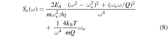
Here EA = 1000ℏ is the SQUID energy resolution, and β and η are the electromechanical energy coupling and energy coupling efficiency from circuit to SQUID with β η = 0.25. More recently, a modification of the SQUID readout was suggested by implementing an LC-bridge transducer, which could potentially overcome limitations of the readout noise (Paik et al. 2016). Mostly to avoid the introduction of high-temperature superconductors in our cryomagnetic concept, which are not well explored for levitation systems, we assume that the system is kept cooled at 9 K. This, of course, can be considered a major hurdle for applications on the Moon, which is why exploration of high-temperature (e.g., 40 K) solutions is necessary.
Comparing the two concepts, the optomechanical system has an advantage at higher frequencies since relatively low laser power can already achieve extremely low readout noise. It is difficult to imagine that SQUID readout noise can be lowered much relative to the spectrum given in Figure 2. The cryomagnetic concept is predicted to have a better performance in the thermal-noise-limited band. This is not only because of the more optimistic assumptions about achievable Q-factors but also because of the fact that energy dissipation in magnetic systems is expected to be dominated by viscous damping.
Generally, it would be possible to combine features of the two concepts to create new concepts. For example, a magnetic levitation could be combined with optical readout. However, we think that the two chosen concepts are the most consistent ones since they either fully exploit the benefit of cryo-temperatures or are fully compatible with any ambient temperature. It is also conceivable that the cryomagnetic concept would work at ambient lunar temperatures, as long as it is deployed in one of the PSRs, where temperatures well below 100 K can be found, and then implementing high-temperature (type II) superconductors.
Needless to say, other instrumental noise exists in these concepts, such as laser-frequency noise, other forms of thermal noise, electronics noise, or coupling to fluctuations of ambient electromagnetic fields, but we believe that these can be suppressed more easily by design and precise engineering. Realizing the targeted Q-value and suspension resonance frequency of any of the two concepts is the main challenge.
4.5. Communication and Positioning
There is an enormous effort to create important communication and positioning infrastructure for future missions to the Moon. One idea that has long been discussed is the usage of the terrestrial GNSS for lunar missions (Delépaut et al. 2020). Another interesting opportunity has emerged with the introduction of microsatellites and CubeSats for interplanetary missions. A CubeSat constellation was proposed to form a Lunar Global Positioning System (Batista et al. 2012). While the first phase of the LGWA experiment would not require such infrastructure, subsequent phases, especially with station deployments on the back side of the Moon, would depend on it for accurate navigation.
In general, deployment at sites without continuous Earth visibility would require a novel data link based on satellites in lunar orbit. In order to estimate the requirements of data transmission systems, we provide an estimate of the total instrument data rate and volume for a phase 1 LGWA array with four stations in Table 1.
Table 1. Calculation of Data Transmission Rates for LGWA
| Parameter | Multiplier | Data | Unit |
|---|---|---|---|
| Signal BW to be sampled | 10 | Hz | |
| Sampling BW (Nyquist) | 20 | Hz | |
| Bits per sample | 16 | ||
| Data rate per seismic sensor | 320 | bits s−1 | |
| Data volume per day per seismic station | 2 × 86,400 s | 55,296 | kbits |
| Total data volume per day | 4 stations | 221,184 | kbits |
Note. BW: bandwidth.
Download table as: ASCIITypeset image
Here we assume to have two horizontal seismic channels per seismic station, and four seismic stations in total. Each seismic channel is sampled at 20 Hz. Based on these numbers, the total data transmission rate would be about 250 Mbits day−1. Such transmission rates can in principle be achieved easily today even with direct transmission of sensors to Earth if power is available. The Lunar Atmosphere and Dust Environment Explorer in lunar orbit contained the Lunar Laser Communication Demonstration, which demonstrated download transmission rates of about 600 Mbit s−1 with a total power consumption of ∼90 W (Boroson & Robinson 2014). More conventional X-band communication can achieve a few Mbits s−1 between Earth and Moon (Zhang et al. 2019), while a ∼4 W X-band transmitter on CubeSats could achieve several × 10 kbit s−1 (Schaire et al. 2017), which would still be enough to transmit the total data volume of LGWA with four stations. Future private Moon satellite constellations under development by Commstar Space Communications in collaboration with Thales Alenia Space or the Lunar Pathfinder by SSTL (Surrey Satellite Technology Limited) will provide both communication and navigation services, which can be used by LGWA to facilitate its development.
5. LGWA Science
5.1. Aspects of Data Analyses
LGWA has a few unique features compared to other detectors, which requires specialized data analysis techniques, which give unique capabilities to this concept:
- 1.LGWA, due to the Moon’s rotation with a period of 27.3 days, has a unique temporal evolution of its antenna pattern among all GW detector concepts.
- 2.
- 3.As shown in Figure 1, LGWA has the characteristics of a resonant bar antenna at frequencies up to 10 mHz and transitions into a broadband detector above 10 mHz.
- 4.
The first point is relevant to the estimation of certain GW signal parameters, especially sky location, provided that the GW signal lasts for long enough as would be the case, for example, with less massive compact binaries including DWD or binary neutron stars (BNSs) at mHz frequencies, and GWs from spinning neutron stars (NSs). In these cases, the observed signal amplitude experiences a temporal modulation, which can be exploited for parameter estimation (Grimm & Harms 2020; Wen & Chen 2010).
The ability of an extended array of seismic sensors to measure polarizations of GWs would benefit parameter estimation. For example, in the case of compact binaries, the degeneracy between extrinsic source parameters like orbital inclination, polarization angle, sky location, and distance can be broken, further assisted by temporal variations in antenna patterns as explained earlier. Furthermore, antipodal pairs of seismometers are the ideal configuration for stochastic GW searches since seismic correlations are expected to be small. In this configuration, the two seismometers have the largest possible distance to each other, and at the same time, the overlap reduction function that describes correlations of GW signals as a function of relative position and orientation is maximal (Coughlin & Harms 2014b, 2014c).
The third point determines what data analysis techniques need to be used. For example, a massive binary black hole (BBH) would ring up normal-mode resonances from low to high frequencies with a well-defined beat (beat in the musical sense). For such signals, below 10 mHz, information can only be extracted from the beat and the loudness of each ring. Less massive binaries below 10 mHz, i.e., binaries with negligible frequency evolution, need to hit the right frequencies, i.e., the normal-mode resonances, and will most likely remain undetected off-resonance. Above 10 mHz, standard data analysis techniques can be applied as known for all broadband GW detectors.
The fourth point in the list emphasizes an important complementarity of LGWA’s role in a multiband detector network, which will be further elaborated in Section 5.6.
5.2. Binaries
5.2.1. Signal Modeling
For the analyses in the following sections, GW amplitudes need to be estimated for various observation and modeling scenarios. Hence, we start with the characterization of a binary inspiral. Solar-mass binaries in the LGWA band move slowly in frequency. This can be characterized by the time it takes the binary to merge (Harms et al. 2013),

where  is the redshifted chirp mass of the binary with component masses M1 and M2, and M⊙ is a solar mass. For solar-mass binaries detectable by LGWA, the redshift z will be small and can be neglected. With a GW signal at fGW = 0.1 Hz, the inspiral time would be reduced to 3 yr.
We have seen that LGWA’s response exhibits sharp peaks in the mHz band. A straightforward estimation of the signal-to-noise ratio (S/N) of a solar-mass binary would be possible if the change in frequency of the signal over a few years’ observation time were significantly smaller than the width of these peaks. In this case, LGWA’s response can be approximated as constant during the full observation (apart from a changing antenna pattern due to the Moon’s rotation). The time a binary spends on a specific normal mode can be calculated from Equation (9) and is given by

where the line width of a mode is Δfn = fn /Qn . Certainly at 5 mHz, the change in frequency is still so slow that one can approximate LGWA’s response as constant over a few years even in the vicinity of a normal-mode resonance. This result is what allows us to use Equation (5) to integrate the S/N of a GW signal over a few years. In real analyses, some necessary changes in signal frequency must be considered, though, for example, related to the orbital motion of the Moon causing Doppler shifts (Astone et al. 2014). For signals at higher frequencies, the S/N must be integrated over a range of frequencies.
Since a large range of masses will be considered in the following sections, inspiral times can vary greatly between different signals, which requires different sets of equations to estimate GW amplitudes and S/Ns. In Section 5.2.2, we estimate GW amplitudes of known solar-mass, compact binaries. For some of them, the orbital inclination angle is known, for others not. If the inclination angle is unknown, we use the inclination-angle- and polarization-averaged, time-domain GW amplitude

where c is the speed of light, G the gravitational constant, and r the luminosity distance of the GW source. The GW frequency fGW is twice the orbital frequency of the binary. For compact binaries where an estimate of the inclination angle ι is available, we use the polarization average

Some GW signals from compact binaries can evolve rapidly in frequency during the observation time as would be the case for DWDs above 0.1 Hz or massive BBHs throughout the entire LGWA band. In this case, a full signal spectrum needs to be calculated in the form of a Fourier domain amplitude. Taking Equation (11), together with results from Allen et al. (2012), we obtain the inclination-angle- and polarization-averaged Fourier amplitude

This equation is used in Section 5.2.4 to evaluate signal amplitudes of massive BBHs.
A convenient method to compare signal amplitudes with detector noise is to convert all spectra into characteristic strain. The characteristic strain hn of detector noise is given by (Moore et al. 2014)

where Sn (f) is the power spectral density of the detector noise. This needs to be confronted with the characteristic strain of GW signals. For signals with negligible frequency evolution, the characteristic strain can be written as

where h is the time-domain amplitude of the GW. Instead, if the signal is given as a Fourier spectrum  , then the conversion into characteristic strain reads

When confronting signal amplitudes with instrument noise in the following, we assume that only one seismometer monitors displacements and that it is optimally located with respect to the propagation direction of the GW.
5.2.2. Known Stellar Binary Systems
We collected from literature the orbital parameters (component masses, orbital period, orbital plane inclination) and estimated distance for a variety of known short-period binary systems in the Milky Way. With this information, we computed the expected characteristic strain hc of the GW emission based on Equation (12). We scaled hc to an assumed observing time Tobs = 5 yr considering that all selected sources are monochromatic in this time interval.
The list of binary systems includes the following:
- 1.The LISA verification binaries from Kupfer et al. (2018, and references therein). The list includes 11 semidetached AM CVn–type systems, four DWDs, and a WD with a hot He-rich companion. It has been suggested that the latter system (open green circle in Figure 8) may evolve to become a Type Ia supernova (SN Ia; Geier et al. 2013) (single-degenerate scenario; see below).
- 2.DWDs with known system parameters from the ESO supernovae type Ia progenitor survey (SPY; Napiwotzki et al. 2020) (double-degenerate scenario).
- 3.The DWDs discovered by the Extremely Low Mass (ELM) Survey, a spectroscopic survey targeting M < 0.3 M⊙ He-core WDs (Brown et al. 2020).
- 4.The close binaries found by the Systematic search of Zwicky Transient Facility data for ultracompact binary LISA-detectable GW source (Burdge et al. 2020). These are mainly DWDs, but also AM CVn systems.
- 5.The ultracompact X-ray binaries (UCXBs) from Chen et al. (2020). UCXBs are low-mass X-ray binaries with ultrashort orbital periods made of an NS and a hydrogen-poor donor star.
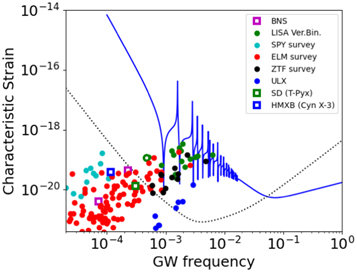
Figure 8. Strength of the GW emission from known short-period binary systems in the Galaxy compared with the expected sensitivity of LGWA (blue line, cryomagnetic) and LISA (black dotted line).
Download figure:
Standard image High-resolution imageLocations of the sources in the hc versus GW frequency plot are shown in Figure 8. In the plot, we included the recurrent nova T Pyxidis (Patterson et al. 2016), another representative of the single-degenerate scenario for SNe Ia; the high-mass X-ray binary (HMXB) Cyg X-3 (Koljonen & Maccarone 2017), likely a BH+WR star; and two short-period BNSs PSR B1913+16 (Hulse & Taylor 1975) and PSR J0737+3039 (Burgay et al. 2003).
The figure shows that up to a dozen known binary systems are bright enough in GWs to be detected by LGWA. UCXBs, while in a suitable frequency range, appear too faint for LGWA. HMXBs are brighter, but they never enter the useful frequency range.
We acknowledge that the list of known binaries is severely biased. WDs are electromagnetically faint, and therefore they can be detected only at relatively short distances. In addition, DWDs can be identified only in favorable conditions, e.g., through the mutual eclipses when our line of sight lies close to the orbital plane.
In fact, recent detailed simulations based on Galaxy structure modeling and binary population synthesis (e.g., Lamberts et al. 2019; Korol et al. 2018) predicted that LISA will be able to resolve signals for up to 105 compact binaries, of which only a small fraction (∼102 events) will also be identified by electromagnetic (EM) radiation.
For LGWA, we propose a similar kind of analysis when an accurate estimate of the array sensitivity will be available. Here, we perform a simple back-of-the-envelope calculation to test the possible performances for a specific science case, which is to identify the progenitors of SNe Ia.
5.2.3. The Case of SN Ia Progenitors
SNe Ia have a crucial role in cosmology for the measurement of the Hubble constant (Riess et al. 2019; Khetan et al. 2021) and the discovery of cosmic expansion acceleration (Riess et al. 1998; Perlmutter et al. 1999). Yet, it is still unclear what is the evolutionary path that leads to explosion (Della Valle & Izzo 2020). The standard scenario calls for a thermonuclear explosion of a WD that grows above the Chandrasekhar mass limit. However, there are two different scenarios that can plausibly lead to this event, both involving compact binaries: (a) the merging of two WDs (double-degenerate scenario), or (b) WD mass accretion from a nondegenerate companion, either a main sequence or a red giant star (single-degenerate scenario).
For double-degenerate systems, merging occurs when the system loses angular momentum due to GW emission, while for single-degenerate systems the timescale is set by the stellar evolution clock of the secondary (Greggio 2010). This implies a different distribution of orbital periods for the two scenarios.
In the double-degenerate scenario, the distribution of the DWD orbital periods can be derived knowing the merging time from GW emission using Equation (9). The total number of DWDs in a selected orbital period range (note that only systems with total mass >1.4 M⊙ are relevant) is constrained by the current rate of SNe Ia in the Galaxy: for the current estimate of five SNe Ia for 1000 yr (Li et al. 2011), the total number of DWDs with orbital period below 5 × 10³ s needs to be ∼240,000. Exploiting the fact that the SN Ia rate in the Galaxy is almost constant for a timescale of a billion years (Greggio & Cappellaro 2019), the orbital period distribution can be easily derived assuming a uniform distribution of the merging time.
For the estimate of the expected GW signal distribution we need to know the distance distribution of the DWD systems. For this exploratory calculation, we take that the systems are distributed as the stars in the Galactic disk modeled with an exponential profile with scale R0 = 2.5 kpc.
With these assumptions, we performed a simple Monte Carlo experiment selecting random orbital periods and random distances following the adopted distributions. For each system, we computed hc, the GW characteristic strain, and then selected the systems with hc higher than the expected array sensitivity hn. We also selected the subsample of systems with hc/hn > 7 that we adopt as the limit for resolved sources.
The frequency histogram for the detected sources is shown in Figure 9. We concluded that if double degenerate is the only viable path to SNe Ia, LISA should be able to resolve ∼103 DWDs with total mass >1.4 M⊙, while LGWA is expected to detect ∼102 DWDs. Considering that the minimum period for the single-degenerate scenario is 1.2 hr (Davis et al. 2010; Patterson et al. 2016), few, if any, of these systems can be detected with  , and even LGWA would then be able to give a definite answer to the long-standing issue of SN Ia progenitors.
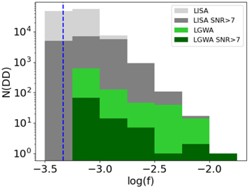
Figure 9. Monte Carlo simulation of the GW frequency distribution for double-degenerate systems in the Galaxy detectable by LGWA and LISA with different detection thresholds. The blue dashed line indicates the expected maximum GW frequency (corresponding to the minimum orbital period) for single-degenerate systems.
Download figure:
Standard image High-resolution imageLGWA’s observation band covers the merger frequencies of DWDs. Figure 10 shows the S/N as a function of the component masses of the binary system at the distance of 1 Mpc observed for 5 yr before the merger. Considering an S/N threshold of 10 for the detection, the merger of the most massive systems can be observed up to 4–5 Mpc. The rate of SNe Ia up to this distance is about 0.02 yr–1 (Li et al. 2011). Even if the probability of a joint detection is low, detecting a GW signal from the DWD merger, together with the optical or high-energy emission of an SN Ia, has an enormous scientific impact to shed light on the progenitor of an SN Ia and for cosmological studies (e.g., Maselli et al. 2020). Furthermore, the probability of a joint detection can increase using SNe Ia exploded within 10 Mpc to drive the GW search of LGWA data as done using gamma-ray bursts or optical core-collapse SNe for the LIGO and Virgo data (e.g., Abbott et al. 2020a).
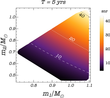
Figure 10. S/N as a function of the component masses of the binary system of WDs at the distance of 1 Mpc observed for 5 yr before the merger. Dashed curves correspond to configurations of constant S/N. The WD masses are chosen to fall within the range where the coalescence may lead to an SN Ia event (Postnov & Yungelson 2014).
Download figure:
Standard image High-resolution imageA prompt association of GW signals from double-degenerate systems with SNe Ia could be achieved by the coincident detection of short-lasting X-ray/gamma-ray signals from a shock breakout (SBO; Colgate 1974). The characteristics of SBO signals, i.e., duration, temperature, and luminosity, strongly depend on the fundamental properties of an explosion, including the size of the progenitor (or an extended region such as wind or debris), its mass, and the total energy of an explosion (Budnik et al. 2010; Katz et al. 2010; Nakar & Sari 2010, 2012; Piro et al. 2009). Particularly for SNe Ia, it is yet unclear whether the SBO is relativistic or Newtonian, since the velocity of the shock front strongly depends on the radius of a breakout. In a single-degenerate model, this radius is expected to coincide with a WD of size ∼1000 km, which would produce a 10 ms flash of low-luminosity ∼1044 erg s−1 MeV photons by relativistic SBO (Nakar & Sari 2012). In a double-degenerate model, the optical depth of the progenitor surroundings could cause a delay of the SBO at ∼1011–1012 m, which corresponds to a Newtonian or sub-relativistic SBO (Fryer et al. 2010). In this case, the expected signal would be much longer (∼103 s), brighter (∼1047 erg s−1), and at softer energy bands (∼50–200 keV) (Nakar & Sari 2010). The brief initial flash of SBO is followed by its fainter cooling tail, which constantly softens and can be observed in soft X-rays and in the UV range. With respect to the optical band, the advantages of detecting the SNe Ia through the SBO are the shorter delay between the GW signal and the electromagnetic signal and the fact that the high-energy emission does not suffer from dust absorption. Large field-of-view satellites observing in the X-rays, such as Einstein Probe (Yuan et al. 2015), SVOM-ECLAIRs (Wei et al. 2016), and the mission concept THESEUS (Amati et al. 2018), are expected to operate in the next decade.
5.2.4. Massive and Supermassive Black Hole Binaries
There is a clear consensus from the observations that the majority of massive galaxies should harbor a central massive BH (MBH, with masses from few × 105 to 1010 M⊙), whose evolution is deeply intertwined with their host (Kormendy & Richstone 1995; Ferrarese & Merritt 2000; Häring & Rix 2004; Kormendy & Ho 2013). Following the current ΛCDM cosmological paradigm, galaxies grow hierarchically through minor and major mergers (Hopkins et al. 2005; Springel et al. 2005). As these BHs share a symbiotic relation with their host galaxy, they should play a significant role during galaxy mergers. Indeed, during a galaxy encounter, the dark matter, gas, and stars of both galaxies form a common envelope around the two BHs, which undergo a process called dynamical friction (e.g., Sesana 2010; Dosopoulou & Antonini 2017). Here the interactions between the BHs and the surrounding matter drag the two BHs toward the center of the new common galactic envelope. Eventually, the two BHs will bind in a binary system with subparsec-scale distance (e.g., Begelman et al. 1980) and emit continuous GWs in the frequency range f ∼ 1–100 nHz. Despite the significant difficulties in observing these kinds of binary systems, several candidates have been proposed by using both optical (e.g., Graham et al. 2015a, 2015b; Charisi et al. 2016) and X-ray observations (Severgnini et al. 2018; Serafinelli et al. 2020). The emission of GWs from the binary will affect the binary period, shrinking their distance at every cycle until they eventually merge (e.g., Dotti et al. 2012; Mayer 2013; Colpi 2014).
The gravitational event from the orbital, merger, and ring-down of the two BHs is in principle observable by low-frequency GW observatories. To assess the observability of these sources with LGWA, we produced waveforms of several binaries (see Figure 11) using the PhenomB template (see Section 5.4 for details). A binary system with M1 = 5 × 10⁶ M⊙ and M2 = 4 × 10⁶ M⊙ at a distance of d ∼ 2 Gpc and a closer system with M1 = M2 = 5 × 10⁵ M⊙ at d = 50 Mpc are both shown in Figure 11. Both these systems have extremely high S/N (≫ 10), and therefore LGWA will be able to follow part of the orbital phase, as well as the merger and ring-down of a coalescence in the mass range M ≲ 107 M⊙, even at large redshift. In fact, considering a detection threshold of S/N ∼ 10, a system with M1 = M2 = 5 × 10⁵ M⊙ can be observed up to z ≃ 3. Figure 12 shows the S/N as a function of the source-frame total mass of these binaries and of the redshift (or of the luminosity distance following Adams et al. 2016).
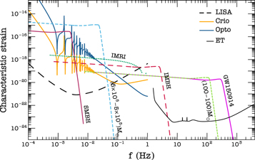
Figure 11. Characteristic strain for various sources. The amplitude is modeled using the PhenomD template in the frequency domain, including post-Newtonian corrections (Husa et al. 2016; Khan et al. 2016). The SMBH system is positioned at a luminosity distance of ∼1.7 Gpc (S/N = 500), the IMBH at a distance of ∼2 Gpc (S/N = 50), and the IMRI at ∼830 Mpc (S/N = 100). The GW150914-like system and the (100–100) M⊙ are positioned at a luminosity distance corresponding to an S/N = 10, i.e., ∼160 and ∼412 Mpc, respectively.
Download figure:
Standard image High-resolution image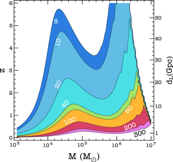
Figure 12. Coalescences of massive and supermassive BBHs. The contours of constant S/N are shown as function of total source-frame mass, M, and of redshift, z (left axis), and luminosity distance, dL (right axis), considering binaries with constant mass ratio among the component masses of 0.2.
Download figure:
Standard image High-resolution imageIt is also very interesting to discuss the implications for the EM observations of massive binaries of a possible LGWA detection, and vice versa. This is particularly relevant because LGWA will have a sky localization, allowing us to point at the emitting source right after the GW detection. The only known type of astrophysical objects powered by an MBH are active galactic nuclei (AGNs). AGNs are powered by the accretion of matter in a disk around an MBH. Such an accretion disk is responsible for the optical and UV emissions, which may exceed the one emitted by the entire host galaxy. Additionally, a hot electron plasma in the region closest to the BH, the so-called corona, up-Comptonizes the UV photons, emitting X-rays (Haardt & Maraschi 1991, 1993). When there is a massive BBH system, the physics related to the accretion disk becomes more complex. In fact, simulations suggest that the two BHs will excavate a cavity inside a circumbinary disk, and the accretion will occur by means of two minidisks, surrounding each of the BHs (e.g., Hayasaki et al. 2008; Noble et al. 2012; d’Ascoli et al. 2018). While the circumbinary disk is responsible for the optical emission, UV photons and X-rays are likely emitted by the minidisks and the coronas; therefore, X-rays are one of the most promising tools to identify binary systems by means of their EM signal. Before the coalescence, as these emissions are produced in the minidisks, a periodic modulation in the UV and X-ray light curves might be expected. An additional feature that may arise is a double-peaked Fe Kα emission line. This Fe emission line is the superposition of the two Fe emission lines arising from each of the minidisks, which are Doppler shifted owing to the orbital motion (e.g., Popović 2012; Sesana et al. 2012; Roedig et al. 2014; McKernan & Ford 2015; Farris et al. 2014; Haiman 2017). Finding these features in the X-rays would be crucial to assess the abundance of MBH merging events in the universe, and, possibly, they would allow us to predict low-frequency BH merger GW signals. In fact, simulations show that this configuration holds until a few orbits before the coalescence (Tang et al. 2018). The EM counterparts of both the merging and ring-down phases are currently unknown and represent an exciting challenge of low-frequency GW astronomy.
5.3. Spinning Neutron Stars
The latest releases (ver. 1.64) of the Australia Telescope National Facility (ATNF) catalog (Manchester et al. 2005) and of the McGill Online Magnetar catalog (Olausen & Kaspi 2014) contain in total 1045 NSs spinning at a period in the 0.04–1.5 Hz range. Most of them (1021) are “ordinary” radio pulsars, the rotational pace of which can be easily monitored in the electromagnetic band by using the procedure of the pulsar timing (e.g., Possenti & Burgay 2016). Another 24 objects belong to the category of the so-called magnetars (Mereghetti et al. 2015), the rotational parameters of which are mostly determined via timing observations in the X-ray band. At the present level of knowledge, none of these NSs are included in a binary system.
All these NSs undergo a secular spin-down, which is commonly believed to mostly arise from the conversion of rotational energy (for the ordinary radio pulsars) and of magnetic energy (for the magnetars) into radiation and particle acceleration.
However, if the NS possesses a nonzero mass quadrupole moment Q22, and assuming polarization properties in agreement with the predictions of general relativity (GR), the rotation of the NS also generates the emission of GWs, which might be partly responsible for the total energy loss, hence playing a role in the observed slowdown of these objects (e.g., Zimmermann & Szedenits 1979). In particular, in the simplest picture, the GWs are emitted at a frequency fgw = 2fsp, where fsp is the spin frequency of the NS. On a theoretical ground, the detailed GW frequency spectrum could be more complex, including also emission at the same rotation rate of the star, as well as a small modulation about both the mentioned frequencies if the NS undergoes free precession (e.g., Zimmermann & Szedenits 1979; Jones & Andersson 2002). However, the strongest GW signal is expected to be the one at twice fsp (e.g., Jones 2015), and we will only focus on that for the purpose of this analysis.
In all cases, the fractional variations in the spin rate of these objects are small over a decadal timescale (10−9–10−3 for ordinary radio pulsars, 10−7–3 × 10⁻² for magnetars). Once the barycentric corrections are applied (i.e., the effects of the combined rotational and orbital motions of the Moon are removed), the expected GW emission can then be considered quasi-monochromatic. Even if the slowdown of some of these sources can experience irregularities (e.g., glitches and rotational noise; e.g., Lyne & Graham-Smith 2012), dedicated electromagnetic campaigns are able to compensate for that and suitably follow the rotational phase for the majority of the ordinary radio pulsars. In practice, the availability of electromagnetic information provides the possibility to integrate the GW signal associated with those NSs over multiyear-long intervals. This holds true also for the population of the bright steady emitting magnetars. Only for the subclass of the transient magnetars can the X-ray luminosity during the quiescent phase go below the threshold for monitoring their rotational behavior. In this case their putative GW signal could be optimally integrated for the duration of the bright phases only, typically lasting of order months.
All the considerations above suggest to investigate whether any potential targets for LGWA could be found in the mentioned populations of NSs.
In the absence of any precession, the amplitude h0 of the GWs released by a triaxial NS spinning around a principal axis (assumed to be the z axis), due to a mass quadrupole Q22 ≠ 0, is (e.g., Aasi et al. 2014)

where, for the sample of NSs under consideration, the distance dkpc in units of kpc lays in the range of 0.11–59.7 and is measured with typical maximum uncertainty of about 50%. The spin frequency in Hz, fsp,1, is in the range of 0.04–1.5 and is measured with negligible uncertainty with respect to the other parameters in the equation above. The value of the component Izz along the spin axis of the moment-of-inertia tensor ellipsoid results from theoretical calculation: although it is dependent on the NS mass and the adopted equation of state, the predicted values Izz,45 span a small range of about 1–3 when expressed in units of 1045 g cm2.
The most uncertain parameter is the ellipticity (expressed in units of 10−6 in the equation above), which is defined on the basis of the true moments of inertia Ixx
and Iyy
about the other two principal axes x and y (left part of the equation below), and which also relates to the mass quadrupole moment Q22 according to the right part of the following equation (e.g., Aasi et al. 2014):

The LIGO and Virgo collaborations have investigated the case of 221 NSs, searching for GW signals at frequencies above 10 Hz (Abbott et al. 2019c, 2020b). The lack of any detection makes it possible to constrain the value of the ellipticity for that sample of rapidly spinning pulsars. The smallest observed upper limit is −6 ∼ 6 × 10⁻³, measured in a pulsar spinning at about 350 Hz, in the frequency interval for which aLIGO had the best sensitivity. The upper limits to the ellipticity scale linearly with those on the GW amplitude (i.e., with the sensitivity at a given frequency, which gets worse below 100 Hz in the case of the aLIGO experiment), as well as with
 . Therefore, when looking at slower-spinning targets, upper limits on
 −6 become much less constraining, i.e., 1–103. For instance, Abbott et al. (2019c) found
−6 < 10 and
−6 < 76 for the Crab and the Vela pulsar, respectively.
The latter constraints are close to the theoretical predictions (suggesting  in the interval 1–10) about the maximum values of the ellipticity associated with an NS of mass 1.2–2.0 M⊙ for a wide range of equations of state (Johnson-McDaniel & Owen 2013) and in the absence of a significant magnetic energy stored inside the NS. Hence, in Figure 13 we adopted a fiducial maximum value
  in order to plot the most optimistic GW amplitudes that we can get from our sample of spinning NSs, supposing that they do not contain ultrastrong magnetic fields or exotic particles. Those amplitudes are compared with the estimated sensitivity of LGWA to quasi-monochromatic GW signals, assuming an integration time of 5 yr and an S/N threshold γ = 5 (see Equation (5)).
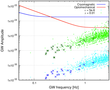
Figure 13. Amplitude of the expected GW signals vs. the GW frequency for the sample of the NSs listed in version 1.64 (2020 October) of the ATNF catalog (https://www.atnf.csiro.au/people/pulsar/psrcat/) or in the McGill Online Magnetar catalog (http://www.physics.mcgill.ca/~pulsar/magnetar/main). All the reported NSs have a known distance and spin at rotational frequencies in the range of 0.04–1.5 Hz. Two values for the ellipticity (expressed in units of 10−6) have been applied:
−6 = 5 (cyan circles and blue stars) and
−6 = 104 (green circles and dark-green stars). The value of the component of the moment-of-inertia tensor ellipsoid along the spin axis Izz,45 is set equal to 1 in units of 1045 g cm2 (see text). In particular, the sample of the so-called “magnetars” is represented with stars, whereas circles are associated with the other NSs in the sample. The predicted sensitivity curves of LGWA are also reported for two different designs of the detector: optomechanical (solid red line) and cryomagnetic (solid blue line). They are calculated assuming an integration time of 5 yr and a minimal S/N for a fiducial detection equal to 5.
Download figure:
Standard image High-resolution imageNone of the selected targets seem suitable to be detected by LGWA, under the aforementioned hypothesis. We also note that the adopted value of  is maybe even too optimistic on an astrophysical ground, in the absence of a strong magnetic field inside the NS. In fact, using a hierarchical Bayesian approach, Pitkin et al. (2018) combined data from individual sources observed during LIGO’s S6 run in order to derive an upper limit of ∼5 × 10⁻² for the mean value of the distribution of
 −6, suggesting that (at least the bulk of) the pulsar population is not strained to its maximum possible value of the ellipticity.
Perspectives for a detection with LGWA might significantly improve if one accounts for the possible role played by a strong magnetic field buried in the interiors of some of the observed NSs (Dall’Osso & Perna 2017; Lander & Jones 2018). Frieben & Rezzolla (2012) calculated that, for a favorable magnetic field topology, internal toroidal magnetic fields of order 1015 G (in the ballpark of the observed values of Bp, the external magnetic field measured at the pole of the “magnetars”) are able to deform a typical 1.4 M⊙ NS to ellipticity values reaching −6 = 100. Moreover, when the internal toroidal component dominates the total magnetic energy budget of the NS, the value of
−6 scales as
 (Ciolfi & Rezzolla 2013), in principle generating magnetic deformations of the NS up to
 −6 = 103 for internal magnetic fields of order 1016 G and up to
−6 = 105 for the maximum allowed B-field strength of ∼1017 G.
Large values for the ellipticity in the condition of maximum strain  can also be approached if some NSs are indeed containing exotic particles (Johnson-McDaniel & Owen 2013), as is the case for the putative “hybrid” stars (i.e., stars having a hadron–quark mixed phase lattice in their core; e.g., Owen 2005), and
  can be sustained by elastic deformations in putative solid quark stars (Johnson-McDaniel & Owen 2013).
In view of these theoretical investigations, we also report in Figure 13 the expected GW amplitudes for our sample in case −6 = 104. In this case there appear to be a handful of potential targets, which could be representative of a small subgroup among the observed NSs, which are endowed with a huge internal magnetic field and/or comprise exotic particles. Despite this admittedly being the most favorable predictable situation, it is interesting to note that LGWA would be the sole instrument capable of discovering such intriguing objects in the mentioned frequency range, since LISA is not expected to have the required sensitivity.
5.4. Fundamental Physics
The low-frequency/long-wavelength GW signals observed by LWGA represent a promising opportunity to study fundamental physics. LGWA is expected to detect sources in a wide range of masses, which will allow us to test the nature of gravity in the strong-field regime and to challenge GR predictions (Berti et al. 2015). Observations by LGWA will be independent and complementary to those obtained by current and future ground-based interferometers (Sathyaprakash et al. 2019; Perkins et al. 2021), leading to searches of possible hints of new physics in a different class of sources. Some of the science cases that will benefit from LGWA observations include (i) tests of non-GR signatures within the GW generation and propagation mechanisms, (ii) tests of the nature of BHs and of the existence of new degrees of freedom that modify the gravitational interaction and/or of exotic states of matter, (iii) probes of dark matter and of dark energy models, and (iv) characterization of the environment in which compact binaries evolve and merge. We refer the reader to Yunes & Hughes (2010), Berti et al. (2018b, 2018a), Barack et al. (2019), Berti et al. (2019), Cardoso & Pani (2019), and references therein for a detailed discussion on these and further fundamental physics topics relevant for the frequency range in which LGWA is sensitive. Hereafter, instead, we will focus on two specific classes of tests, studying the actual constraints that LGWA will be able to infer on GR modifications, based on the cryomagnetic noise spectral density described in the previous sections.
As a first science case we focus on model-independent tests of gravity in the inspiral part of the signal emitted by compact binaries. Theory-agnostic approaches allow us to study possible GR modifications, testing the validity of the post-Newtonian structure of the GW signals. We consider here the parameterized post-Einsteinian framework (ppE; Yunes & Pretorius 2009), which introduces shifts within both the amplitude and the phase of the waveform, which can be measured using GW data. Constraints on such parameters can be mapped to bounds on the fundamental couplings of specific theories of gravity, alternative to GR (Yunes & Siemens 2013). This approach roots into the well-known parameterized post-Newtonian (ppN) formalism developed by Will and Nordtvedt (Will 1971a, 1971b; Nordtvedt & Will 1972; Will & Nordtvedt 1972), and it is analogous to the parametric analysis routinely performed by the Virgo/LIGO collaboration (Abbott et al. 2019b, 2016b).
The top panel of Figure 14 shows the projected constraints obtained by LGWA using a Fisher matrix analysis (Sathyaprakash & Schutz 2009), for modifications of the GW phase at different PN orders, for three type of sources: (i) intermediate mass ratio inspirals (IMRIs) with masses (m1, m2) = (105, 103) M⊙, (ii) intermediate-mass BHs (IMBHs) featuring (m1, m2) = (5, 4) × 103 M⊙, and (iii) supermassive BH (SMBH) binaries with (m1, m2) = (5, 4) × 106 M⊙. The GW signal is modeled through the PhenomB template in the frequency domain for nonprecessing spinning BHs (Ajith et al. 2008, 2011) augmented by the ppE phase shift, with Newtonian amplitude averaged on the source orientation and distance set in order to have an S/N equal to 100, 50, and 500, for IMRIs, IMBHs, and SMBHs, respectively, which correspond to a luminosity distance of d ≃ (827, 1954, 1698) Mpc. For all binaries the dimensionless spin parameters are fixed to (χ1, χ2) = (0.7, 0.9). The bounds scale as the inverse of the S/N. Therefore, the values shown in Figure 14 can be easily rescaled to any value of the S/N.
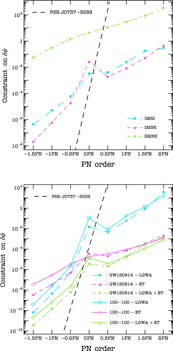
Figure 14. Top: constraints on agnostic deviations from GR in the inspiral phase of different classes of compact binaries. The horizontal axis shows the post-Newtonian order of the waveform modification. The dashed black line identifies the agnostic constraints inferred form binary pulsar observations (Yunes & Hughes 2010). Regions above the curves are excluded by observations. Bottom: same as the top panel, but for a system with the same masses and spins of GW150914 and a binary with m1 = m2 = 100 M⊙, observed by LGWA and by a 3G ground-based detector like the Einstein Telescope. Signals are integrated for 5 yr before the end of the inspiral phase, as defined in Ajith et al. (2008), and the luminosity distance is fixed to have an S/N of 10 in LGWA.
Download figure:
Standard image High-resolution imageFor comparison, we also show similar constraints inferred from binary pulsar observations in the electromagnetic band (Yunes & Hughes 2010), with the region above each curve being ruled out by observations. For PN coefficients ≳0, projected constraints by LGWA will be stronger than those obtained by pulsars. For negative PN corrections, which are more relevant for systems with large orbital separation, i.e., small frequencies, LGWA will also be able to derive strong bounds on the GW phase shifts, although those coming from binary pulsars will still be dominant. However, it is worth remarking that the single-case scenario analyzed here will also benefit from multiple GW observations, which can be easily combined into this approach in order to further lower the bounds on the phase shifts. For low-mass sources, LGWA can also be exploited to perform a multiband test of GR. The bottom panel of Figure 14 shows indeed the constraints on a (i) GW150914-like system and (ii) a (100–100) M⊙ binary with (χ1, χ2) = (0.7, 0.9), observed both by LGWA and by a 3G detector like ET (Punturo et al. 2010). This analysis shows how the synergy between LGWA and future ground-based detectors can narrow down the bounds on the GR deviations on a wide range of PN orders, active at both lower and high frequencies.
LGWA will also be able to test a fundamental pillar of GR, i.e., the uniqueness of the Kerr nature (Hansen 1974), through observations of BH quasi-normal modes (QNMs). The latter are completely determined, in GR, by the mass and spin angular momentum of the ringing object, while solutions beyond GR may feature a nontrivial dependence on extra parameters (Berti et al. 2015). Any change in the QNM frequencies ω and damping times τ of rotating BHs can be parameterized as

where δ ω and δ τ are GR deviations that can be constrained by actual GW signals (Gossan et al. 2012; Meidam et al. 2014; Carullo et al. 2018; Maselli et al. 2020). We explore here the possibility of LGWA to perform a null test of GR, i.e., assuming δ ω = δ τ = 0, by constraining the QNM shift parameters using multiple observations of the BH fundamental ℓ = m = 2 mode (Maselli et al. 2020). Figure 15 shows the probability distribution inferred on δ ω and δ τ, using a Bayesian approach (Maselli et al. 2020), with an increasing number of detected modes, from binaries with component masses and spins uniformly drawn between (106, 107) M⊙ and (−1, 1), respectively. For the sake of simplicity we assume that the S/N of each mode is equal to 100. LGWA can potentially narrow GR deviations with good accuracy, on both frequencies and damping times, with 100 events leading to constraint ∣δ ω∣ ≲ 7 × 10⁻⁴ and ∣δ τ∣ ≲ 4 × 10⁻³ at 90% confidence level. Here time is expressed in units GM/c3, with M being the mass of the BH remnant.

Figure 15. Posterior probability distributions for GR deviations within the QNM spectrum of rotating BHs observed by LGWA, as a function of the number of observed events. We assume that only the fundamental ℓ = m = 2 mode is detected, and that the S/N of each event is fixed to 100. Vertical bars identify 90% confidence intervals. Time is measured in units of GM/c3.
Download figure:
Standard image High-resolution imageA unique ability of LGWA as a single detector to test GR originates from the Moon’s spherical shape and the fact that seismometers can be distributed, in principle, over its entire surface. This idea was first published for the concept of a spherical, resonant detector (Wagoner & Paik 1976; Bianchi et al. 1996), and it requires an estimation of polarization content of a GW field. GR predicts that GWs can only exist as tensor modes, but other metric theories might give rise to scalar and vector modes. In total, six independent polarization modes can exist in metric theories. Assessing whether a GW signal is consistent with a pure tensor mode constitutes a GR test. As demonstrated for the Virgo/LIGO detector network, the test can be done on stochastic GW backgrounds (Abbott et al. 2018b) or on individual signals, such as for the BNS merger GW170817 (Abbott et al. 2019b). In all cases so far, no evidence for scalar and vector modes was found.
5.5. Lunar Science
The Moon is a complex differentiated planetary object and the only body besides Earth on which extensive seismological experiments have been carried out with success. In fact, Apollo missions installed a network of four three-component, long-period seismometers on the Moon (two other stations were short-lived), which revealed more than 12,500 seismic events over a 9 yr period (Nakamura et al. 1981; Khan et al. 2013). Even if our knowledge of the Moon has been significantly increased with Apollo missions, much remains to be explored and discovered, regarding both the origin (and history of the Earth–Moon system) and the internal structure. The absence of plate tectonics made it possible that well-defined accretion and geological evolution records are preserved, unlike on Earth.
Several models have been proposed in order to explain the origin of the Moon: co-accretion (e.g., Thomson 1862), fission (e.g., Durisen & Scott 1984), and capture (e.g., Bok 1952), but all these scenarios suffer from serious flaws. The current accepted model is the so-called “Giant impact,” which implies the collision of the proto-Earth with a Mars-size differentiated object in the early solar system (Canup 2004). This model would be able to explain why, for example, the Moon does not have a large iron core and why it has exactly the same oxygen isotope composition as Earth. The interior structure is probably differentiated into a crust, a mantle, and a core (see Figure 16), even if the degree of differentiation is low as attested by its nondimensionalized moment of inertia, i.e., 0.393 (Williams et al. 2014). As a comparison, Earth has a nondimensionalized moment of inertia of 0.33 (Williams 1994).
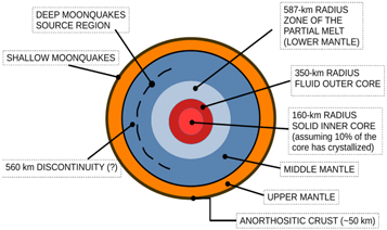
Figure 16. Schematic of the internal structure of the Moon. The Moon’s radius is 1737 km.
Download figure:
Standard image High-resolution imageThe crust has a thickness of about 50 km and an anorthositic composition, containing elements like O, Si, Fe, Al, and also long-lived radiogenic elements (Garcia et al. 2019). The mean density is about 2500 kg m−3 with a porosity of 12%, which probably increases in a significant way with depth (Besserer et al. 2014). The composition of the mantle is predominantly made of olivine, orthopyroxene, and clinopyroxene (Toksöz et al. 1974; Hood & Jones 1987), more iron-rich than on Earth. The uppermost mantle has a density of about 3200 kg m−3 and a porosity of 6%, with a thermal gradient of 0.5–0.6°C km−1 (Garcia et al. 2019). Seismic data suggest a discontinuity at about 560 km from the surface. At a depth of about 1150 km, instead, seismic waves are strongly attenuated in a region that is partially melted and probably represents the core–mantle boundary (Nakamura 2005; Weber et al. 2011). The core is small (≃350 km; Wieczorek 2006), liquid in the external part, and solid in the internal part: this configuration is required to explain the lunar laser ranging (LLR) measurements of the Moon’s pole rotation (e.g., Williams et al. 2001). However, there are several estimates of the size and density (composition) of the core derived from geophysical data and modeling; please see Table 1 of Garcia et al. (2019) for a complete review. Even if the composition of the core is not well constrained, it could be composed mostly of metallic iron alloy and a small quantity of sulfur and nickel (Garcia et al. 2019). As discussed before, the key information about the internal structure comes from seismic studies. Several lunar seismic models exist; see Figure 17. These models have greatly increased our knowledge about the deep lunar interior, for example, the mantle density structure, but they have substantial difficulty in well defining the core size, since the core is very small.
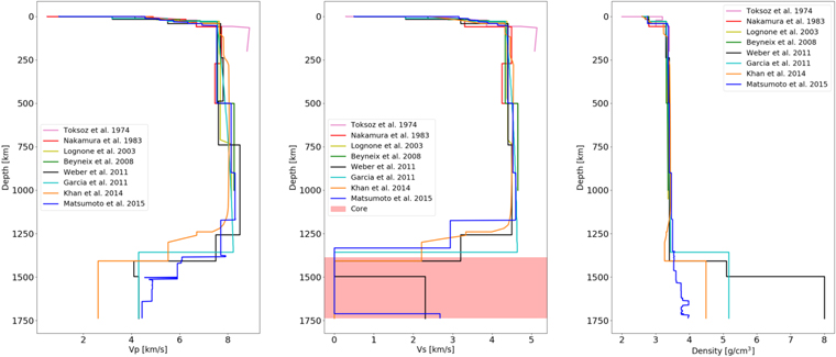
Figure 17. Comparison of several seismic velocity models (left and middle panels for compressional-wave speed Vrmp and shear-wave speed Vs) and density (right panel). In the middle panel, we identify also the core, assuming a size of ≃350 km (Wieczorek 2006). Data for these plots are taken from Garcia et al. (2019). These models are important for the calculation of normal modes and their response to GWs. The references in the plot legends are Toksöz et al. (1974), Nakamura (1983), Lognonné et al. (2003), Gagnepain-Beyneix et al. (2006), Garcia et al. (2011), Weber et al. (2011), Khan et al. (2014), and Matsumoto et al. (2015).
Download figure:
Standard image High-resolution imageSeismicity on the Moon can be classified in three main categories: the deep moonquakes, occurring in the so-called “nests” (at a depth between 700 and 1100 km), with typical magnitudes of around 2, correlated with the lunar tides; the shallow moonquakes are stronger (up to magnitudes of 5.5 on the Richter scale) than the deep moonquakes, but relatively rare and occurring at depths between 50 and 200 km and not connected with geological or geographic features (e.g., Nakamura et al. 1979); finally, moonquakes can also be caused by meteoroid impacts.
5.6. Synergy with Other Detectors and Multiband Observations
Synergy emphasizes the mutual benefit from combined observations with other GW detectors or with electromagnetic facilities to improve their combined science case. The science case outlined in the previous sections contained elements of synergy focused mainly on multimessenger observations. In the following, we briefly discuss the synergy between GW detectors.
If a few GW detectors are sensitive in the same band, then a well-known example of synergy is the localization of a GW source in the sky (Wen & Chen 2010; Abbott et al. 2017a). The source localization of the BNS merger GW170817 was essential for the ensuing multimessenger campaign (Abbott et al. 2017b). Estimation of other parameters like distance and inclination angle of a compact binary can also improve when data from several detectors are combined. For LGWA, it is hard to make any predictions whether it will observe with another detector with overlapping observation band, but the space-borne detector LISA is a possible example (provided that LGWA can be realized on a similar time line). Taking into account that LGWA has interesting sky localization capabilities due to its more rapid rotation (27.3 days compared to 1 yr for LISA), it can be expected that it would significantly improve parameter estimation of some GW signals compared to LISA alone.
If GW detectors are sensitive in different frequency bands, then joint multiband observations can be carried out (Sesana 2016). Signals from compact binaries evolve in frequency and can sweep over various bands. For example, solar-mass compact binaries or intermediate-mass BBHs can inspiral from the LGWA band to the band of ground-based GW detectors within a few years determined by Equation (9). This can lead to improved parameter estimation accuracy (Isoyama et al. 2018; Grimm & Harms 2020). We have seen in Section 5.4 as well that multiband observations can lead to improved tests of GR. Concerning LGWA, the case of inspiraling BNSs is very interesting. If first observed at frequencies above 0.1 Hz, these would have merger times short enough—up to a few years—to make multiband observations with ground-based detectors possible. LGWA could issue an early warning to ground-based detectors of such highly interesting events (Chan et al. 2018).
6. Conclusions
In response to the ESA Call for Ideas, “Exploring the Moon with a large European lander,” a concept for a GW detector on the Moon—the LGWA—was submitted (Harms et al. 2020c). It is based on the early idea of Joseph Weber to monitor surface vibrations of the Moon caused by GWs. A near-term opportunity to explore lunar environmental parameters of the Moon important to LGWA is provided by NASA’s Moon exploration program Artemis, which includes human landings starting with Artemis III and several robotic landings. An Artemis III science white paper was submitted to propose the deployment of a lunar geophysical station in one of the permanent shadows of the south pole, which we identified as a potentially very attractive location of a future LGWA station deployment (Harms et al. 2020a).
In this paper, we have described the LGWA concept in greater detail. We have shown that LGWA would have a broad science case as an independent GW detector and in synergy with other detectors. The science can be enriched by electromagnetic observations allowing a multimessenger astronomy of sources such as inspirals and mergers of WD binaries; supermassive, massive, and intermediate-mass BBHs; and potentially, although less likely, spinning NSs. Furthermore, LGWA would contribute to the geophysical exploration of the Moon, and vice versa, GW analyses of LGWA data crucially rely on the availability of accurate models of the Moon’s internal structure.
Central to the concept is a seismometer whose sensitivity must approximately match the displacement sensitivity of the LISA Pathfinder mission, which was, however, demonstrated under conditions of near freefall. Achieving similar performance under the influence of the Moon’s gravity, which requires a suspension mechanism of the seismometer’s test mass, is a nontrivial feat.
Operating seismometers of such sensitivity would require an extremely low level of seismic disturbances, which cannot be found in natural, terrestrial environments. Since the instrument performance needs to be demonstrated ahead of a deployment on the Moon, the development of a seismic platform stabilized actively using high-end seismic sensors of ground displacement and rotation is necessary. Such platforms would ideally be located in underground environments to profit from a straightforward reduction of the seismic input.
An opportunity for the required technology developments for LGWA is the strong overlap with technologies required for future, terrestrial GW detectors like ET and Cosmic Explorer. Platforms with actively suppressed seismic motion have already been realized as part of a seismic isolation system for the Advanced LIGO detectors (Matichard et al. 2014, 2015), but their performance needs to be improved significantly for LGWA especially to extend the noise suppression toward mHz frequencies. Also, increasing the sensitivity of seismometers beyond what is currently available commercially or in research laboratories could equally lead to improved performance of seismic isolation systems in future GW detectors, enabling the most optimistic scenarios of low-frequency, terrestrial GW observations. In this context, development of LGWA technologies has already started.
A.M. acknowledges support from the Amaldi Research Center, funded by the MIUR program “Dipartimento di Eccellenza,” CUP: B81I18001170001. J.H. acknowledges support from PRIN-MIUR 2017 (grant 2017SYRTCN). V.B., R.D.C., P.S., and R.S. acknowledge partial financial contribution from the agreement ASI-INAF n. 2017-14-H.0. E.C., E.B., M.B., M.d.V., A.G., A.P., P.D.A., and E.P. acknowledge support from PRIN-MIUR 2017 (grant 20179ZF5KS). S.C., P.D.A. and G.T. acknowledge funding from the Italian Space Agency, contract ASI/INAF n. I/004/11/4.
Appendix: Meteoroid Background
For a simplified evaluation of seismic waves produced by meteoroid impacts, we assume that the meteoroid flux is stationary and isotropic. We also assume that the impact is in the normal direction to the surface, which means that we can focus on the radial displacement of spheroidal modes. It should be straightforward to extend the calculation to arbitrary angles of incidence, so that meteoroid impacts can excite radial and transverse displacement of spheroidal and toroidal modes.
Each impact event can be represented as a surface point force at angular coordinates θ0, ϕ0. The normal surface displacement at θ, ϕ is determined by a Green’s function, which can be written as the following product (Ben-Menahem 1983):
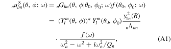
where R = 1.7 × 10⁶ m is the radius of the Moon, y1n
is a radial function characterizing radial displacements of spheroidal normal modes, f(ω) is the Fourier domain amplitude of the radial force exerted by the impact, and  are the scalar surface spherical harmonics. The normalization factor

implies that the Moon is modeled as a laterally homogeneous body (its density ρ0 only depends on the radius). Such models have been used with great success in normal-mode analyses of Earth vibrations. The radial function y3n appearing inside this integral characterizes the transverse displacement of spheroidal modes. This definition of the radial normalization factor is consistent with spherical harmonics in orthonormal normalization:

A different normalization convention is used by Ben-Menahem, which means that numerical factors are not the same when comparing with his work (Ben-Menahem 1983). We now proceed by calculating the power spectral density of background noise n
Slm
(ω) integrating over the Moon’s surface with respect to angles θ0, ϕ0 assuming an isotropic meteoroid shower. In the following, we can omit the angular dependence  of the excited normal modes, since we only need the normal-mode amplitudes. We then obtain

where Sp (ω) is the spectral density of effective pressure fluctuations acting on the Moon’s surface isotropically owing to a steady flux of meteoroids, which also depends on the formation of ejecta, elasticity properties of the impact, and the transfer efficiency of impact energy to the seismic field (typically a small fraction of the kinetic energy of a meteoroid; Lognonné et al. 2009). The last equation has the on-resonance form

The term  depends on the Moon’s internal structure and is of the order of 0.2/M for lower-order quadrupole modes, where M = 7.3 × 10²² kg is the mass of the Moon, so that we can approximate the last equation as

The spectral density of pressure fluctuations is related to pressure rms by  below 1 Hz (Theodorsen et al. 2017), where τ is the average duration of meteoroid impacts henceforth assumed to be τ = 0.1 s neglecting complications like the formation of ejecta.
The effective pressure 〈p〉 produced by meteoroids with flux F and momentum mv is given by

where α is the efficiency of momentum transfer to the seismic field. For our order-of-magnitude estimate, we go with the approximation  , where we use F0 = 10−5 m−2 s−1 for the flux and m0
v0 = 10−3 kg m s−1 for the average meteoroid momentum (Grün et al. 2011), and α = 0.01, which seems to be a generous overestimation of the impact-energy-to-seismic conversion efficiency (Lognonné et al. 2009; Quillen et al. 2019). Note that this expression is independent of the dynamical timescale τ of the impact since we are interested in the average force or pressure, which means that the relevant timescale Δt of momentum transfer ΔP is given by the average time between impacts, which is contained in the meteoroid flux.
, where we use F0 = 10−5 m−2 s−1 for the flux and m0
v0 = 10−3 kg m s−1 for the average meteoroid momentum (Grün et al. 2011), and α = 0.01, which seems to be a generous overestimation of the impact-energy-to-seismic conversion efficiency (Lognonné et al. 2009; Quillen et al. 2019). Note that this expression is independent of the dynamical timescale τ of the impact since we are interested in the average force or pressure, which means that the relevant timescale Δt of momentum transfer ΔP is given by the average time between impacts, which is contained in the meteoroid flux.
It is possible that the total (undirected) momentum transfer onto the Moon is dominated by rare impacts of larger meteoroids, where rare means less frequent than once per Qn /fn , which is about once per day for the lower-order quadrupole modes. With 4π R2 × 1 day = 3 × 10¹⁸ m2 s, we estimate that impacts of meteoroids with mass greater than 1 kg occur less than once per day (Grün et al. 2011). These events need to be treated individually and cannot be considered part of the stationary background noise anymore. As for any other larger seismic disturbance, one needs to exclude the stretch of data containing the large impact event from GW analyses, or attempt a subtraction of the seismic signal from the seismometer data.
Inserting the expression of the surface pressure from meteoroid impacts into Equation (A6), we obtain

Confronting this equation with the on-resonance normal-mode response to GWs, we can say that the effective strain noise in mode n from meteoroid impacts is

where the numerical value depends weakly on the order of normal modes below about 10 mHz according to our simplified response model. The value lies well below the LGWA strain-noise target of 10−20 Hz−1/2. For a full frequency-dependent expression, one needs to include off-resonance response of normal modes as present in Equation (A1) and sum over all modes. Also, the full GW response is required when referring the meteoroid background to effective GW strain noise as done on resonance in Equation (A9). Finally, one needs to keep in mind that the numerical factor in the last equation depends on the order of the normal mode. Still, the on-resonance meteoroid background in the mHz band can be approximated by the formula in Equation (A9).