Abstract
We report on variability and correlation studies using multiwavelength observations of the blazar Mrk 421 during the month of 2010 February, when an extraordinary flare reaching a level of ∼27 Crab Units above 1 TeV was measured in very high energy (VHE) γ-rays with the Very Energetic Radiation Imaging Telescope Array System (VERITAS) observatory. This is the highest flux state for Mrk 421 ever observed in VHE γ-rays. Data are analyzed from a coordinated campaign across multiple instruments, including VHE γ-ray (VERITAS, Major Atmospheric Gamma-ray Imaging Cherenkov), high-energy γ-ray (Fermi-LAT), X-ray (Swift, Rossi X-ray Timing Experiment, MAXI), optical (including the GASP-WEBT collaboration and polarization data), and radio (Metsähovi, Owens Valley Radio Observatory, University of Michigan Radio Astronomy Observatory). Light curves are produced spanning multiple days before and after the peak of the VHE flare, including over several flare “decline” epochs. The main flare statistics allow 2 minute time bins to be constructed in both the VHE and optical bands enabling a cross-correlation analysis that shows evidence for an optical lag of ∼25–55 minutes, the first time-lagged correlation between these bands reported on such short timescales. Limits on the Doppler factor (δ ≳ 33) and the size of the emission region ( ) are obtained from the fast variability observed by VERITAS during the main flare. Analysis of 10 minute binned VHE and X-ray data over the decline epochs shows an extraordinary range of behavior in the flux–flux relationship, from linear to quadratic to lack of correlation to anticorrelation. Taken together, these detailed observations of an unprecedented flare seen in Mrk 421 are difficult to explain with the classic single-zone synchrotron self-Compton model.
1. Introduction
Blazars are a subclass of radio-loud active galactic nuclei (AGNs) with jets of relativistic material beamed nearly along the line of sight (Blandford & Rees 1978; Urry & Padovani 1995) whose nonthermal radiation is observed across the entire spectrum, from radio to γ-rays. Due to Doppler beaming, the bolometric luminosity of blazars can be dominated by very high energy (VHE; >100 GeV) γ-rays. At a redshift of z = 0.031, Mrk 421 is the closest known BL Lac object (de Vaucouleurs et al. 1995) and the first extragalactic object to be detected in VHE γ-rays (Punch et al. 1992). Blazars now comprise the majority source class of VHE extragalactic γ-ray emitters (Wakely & Horan 2008), and while there is much we have learned from multiwavelength data taken over the past 40 years on Mrk 421 and other blazars, there remain many unanswered questions. Indeed, there is still no general agreement on the particle acceleration mechanism within the jet or the location of γ-ray emission zone(s) (e.g., Boettcher 2019). Nonetheless, progress can be made through dedicated campaigns organized simultaneously across as many wave bands as possible (e.g., Aleksić et al. 2015a; Furniss et al. 2015; Ahnen et al. 2018).
The spectral energy distribution (SED) of blazars is characterized by a double peak, while the lower peak is due to synchrotron radiation and the higher peak is generally thought to arise from inverse Compton (IC) upscattering of lower-energy photons off the population of accelerating electrons in the jet (Jones et al. 1974). Hadronic models (Mannheim 1993; Aharonian 2000; Mücke & Protheroe 2001; Dimitrakoudis et al. 2014), or even leptohadronic models (Cerruti et al. 2015), may also be responsible for the second SED peak. The synchrotron self-Compton (SSC) model posits that the seed photons for the IC process are the synchrotron photons from the accelerating electrons (e.g., Ghisellini et al. 1998). Observationally, blazars are classified by the peak frequency of their synchrotron emission; with  Hz, Mrk 421 is deemed a high-frequency peaked BL Lac (HBL; Nieppola et al. 2006).
Blazars exhibit complex temporal structures with strong variability across the spectrum from radio to γ-rays (e.g., Romero et al. 2017 and references therein). Blazar light curves are typically aperiodic with power-law power spectral density (PSD) distributions indicative of stochastic processes (Finke & Becker 2015). Multiband blazar light curves can be punctuated by dramatic flares on timescales from minutes to days where interband correlation is often observed (Acciari et al. 2011; H.E.S.S. Collaboration et al. 2012; Ahnen et al. 2018).
Studying the time-varying characteristics of a source through multiwavelength campaigns can test model predictions of what governs the γ-ray emission and its location within the jet. The standard homogeneous single-zone SSC model of blazar emission employs a single population of electrons that is accelerated in a compact region <1 pc from the central engine (the central black hole driving the jet). The accelerated electrons cool through the emission of synchrotron radiation, then potentially through IC scattering and/or escape out of the accelerating “blob.” The spatial scale of the emission region can be set by the variability detected in the VHE-band observations. Competition between cooling, acceleration, and dynamical timescales that characterize the system can lead to several potential observables, including asymmetries in flare profiles and “soft” or “hard” lags (and accompanying clockwise or counterclockwise hysteresis loops), as described in, e.g., Kirk et al. (1998) or Li & Kusunose (2000).
Much of the previous work with Mrk 421, as well as the ever-growing population of blazars detected by VHE instruments, indicates that most SEDs of HBLs can be described by a single-zone SSC model (Acciari et al. 2011; Abeysekara et al. 2017; Ahnen et al. 2018). As tracers of the same underlying electron population, hard X-rays typically probe the falling edge of the synchrotron peak, while VHE γ-rays probe the falling edge of the IC peak in an HBL with the expectation that these bands will show highly correlated fast variability. However, orphan flares, such as the 2002 VHE flare observed in 1ES 1959+650 (Krawczynski et al. 2004) without a corresponding X-ray flare, provide evidence that one-zone SSC models are too simplistic. The remarkable VHE flare in PKS 2155–304 seen by the High Energy Stereoscopic System (H.E.S.S.) in late 2006 July suggests a need for two emission zones to explain the data (Aharonian et al. 2009). Several recent campaigns on Mrk 421 and Mrk 501 also indicate a preference for a multicomponent scenario (Aleksić et al. 2015b; Ahnen et al. 2017).
Fast flaring events provide another test of the SSC model. Several blazars have been observed to emit VHE flares that vary on timescales of 5–20 minutes (Albert et al. 2007; Aharonian et al. 2009). There is a history of fast flares for Mrk 421 itself, including those reported in Gaidos et al. (1996), Błażejowski et al. (2005), Fossati et al. (2008), and Acciari et al. (2011). These ∼minute timescale flares pose serious issues for single-zone blazar models, as the implied high bulk Lorentz factors required are in tension with the radio observations of these sources (Böttcher et al. 2013; Piner & Edwards 2018). Moreover, the shock-in-jet model suggested to explain knots of material traveling along the jet in radio observations is found to be incompatible with the highly compact emission regions implied by fast flaring episodes detected in blazars (Romero et al. 2017). Indeed, since the majority of blazars are detected during flaring episodes, the erroneous interpretation could be made that a single-zone SSC scenario is responsible for the generic form of the object’s SED. In fact, there may be more than one emitting region at any given time, with one region accounting for “quiescent” or “envelope” behavior, while another region or process may be responsible for a detected flare triggered by a localized event (e.g., magnetic reconnection; Petropoulou et al. 2016). Given the sometimes surprising and dynamical nature of blazars, efforts to coordinate multiwavelength campaigns continue to be important. The results from each campaign provide further clues for modelers to incorporate. For example, highly correlated rapid variability observed between the VHE and optical bands such as described in this work has not been reported before or accounted for in modeling. The observed (or lack of observed) correlated activity between specific bands can discriminate between possible emission mechanisms, and stringent constraints on the sizes and locations of γ-ray emission regions can be set by the flux and spectral variability patterns of blazars (Boettcher 2012).
In this paper, we apply timing analysis techniques, including variability and correlation studies, to the extraordinary Mrk 421 flare recorded in 2010 February by the VERITAS observatory and many multiwavelength partners. During 2009–2010, Mrk 421 was the object of an intense multiwavelength campaign organized by the Fermi Large Area Telescope (Fermi-LAT) collaboration and involving the ground-based imaging air Cerenkov telescopes (IACTs; H.E.S.S., MAGIC, and VERITAS), as well as the Rossi X-ray Timing Experiment (RXTE) and Swift satellites in the X-ray, Swift Ultraviolet/Optical Telescope (UVOT) ultraviolet, and numerous ground-based optical and radio telescopes. Several smaller flares were observed throughout the campaign, including one in 2010 March described in Aleksić et al. (2015b). Here we report on the multiwavelength data set covering the period 2010 February 1–March 1 UT (MJD 55228–55256) with a focus on the giant VHE flare on 2010 February 17 UT (MJD 55244). We note that several other instruments have observed the same flare, including MAXI (Isobe et al. 2010), H.E.S.S. (Tluczykont et al. 2011), HAGAR (Shukla et al. 2012), and TACTIC (Singh et al. 2015).
This paper is organized as follows. In Section 2 we describe the multiwavelength data sets, including the respective methods for analyzing the data presented. In Section 3 we focus on the results from the night of the exceptional flare, including the variability analysis of VERITAS data and results from optical–VHE correlation studies. The results of further multiwavelength studies over the full 2010 February data set are presented in Section 4, including multiwavelength variability studies and VHE–X-ray and high-energy (HE)–X-ray correlation analyses. We conclude with an overall discussion of the results in Section 5.
2. Data Sets and Data Reduction
The multiwavelength light curves covering radio-to-VHE observations around the time of the Mrk 421 2010 February flare are shown in Figure 1. While the light curves in Figure 1 are meant as an overview of available observations, they demonstrate the full breadth of the campaign and show the progression of the flare; more detailed light curves in the various wave bands are considered later in the paper. We summarize the available data sets and present details of the instruments in the following subsections. The data for light curves used throughout this paper are available online.
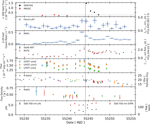
Figure 1. Light curves for multiband observations during the 2010 February portion of the Fermi-LAT–led campaign. From top to bottom: VHE (VERITAS, MAGIC), HE (Fermi-LAT), hard X-ray (MAXI), X-ray (RXTE, Swift-XRT), UV (Swift-UVOT), optical (Abastumani (blue), CRAO (orange), GRT (green), Galaxy View (red), KVA (purple), NewMexicoSkies (brown), Perkins (pink), RCT (gray), and Steward (tan)), and radio (UMRAO 8 GHz (blue stars) and 14 GHz (orange squares), OVRO 15 GHz (green circles), and Metsähovi 37 GHz (red triangles)), including optical polarization observations (Steward Observatory). The light curves are binned by individual observation, except for VHE, HE, and MAXI, which are daily binned. The time of the giant VHE flare is denoted by the dashed vertical line. The dotted horizontal line in the VHE (top panel) denotes 1 CU based on Aharonian et al. (2006). Note that error bars are not visible for several bands due to high statistics. The data behind this figure are available in FITS format. The FITS table has 11 extensions. The MAGIC/VERITAS, Fermi-LAT, MAXI, RXTE, and Swift-XRT are in the first five extensions, respectively. The Swift-UVOT uvw2, uvm2, and uvw1 are in extensions 6–8, while the R-band and radio data follow in the next two extensions. The last extension contains the polarization data.(The data used to create this figure are available.)
Download figure:
Standard image High-resolution image2.1. VHE γ-Ray Observations
The VHE γ-ray data comprise both MAGIC and VERITAS observations. Starting with the MAGIC observatory, data were taken on Mrk 421 between MJD 55234 and 55240 (2010 February 7 and 13), with bad weather preventing further observations. Upon an alert from the campaign that the X-ray state was quite high and variable, VERITAS picked up the observations between MJD 55244 and 55247 (2010 February 17 and 20). As soon as VERITAS began taking Mrk 421 data on MJD 55244, VERITAS observed a remarkable flare in progress with a peak flux of ∼15 Crab Units (CU) above 200 GeV (CU based on Aharonian et al. 2006). Over the next 2 days, VERITAS observed the flux decreasing to the average over the 2009–2010 season, ∼1 CU, which was itself an elevated state (see Acciari et al. 2011). The MAGIC and VERITAS combined VHE γ-ray light curve for Mrk 421 is shown in the top panel of Figure 1 in daily bins for data taken between MJD 55234 and 55247. The VHE data with considerably finer binning are described below in Sections 3.1, 3.3 and 4.3.
VERITAS.—The VERITAS array (Holder et al. 2006; Acciari et al. 2008) is located at 1300 m above sea level in Arizona at the Fred Lawrence Whipple Observatory (31◦ 40′ N, 110° 57′ W) and comprises four Davies–Cotton design telescopes, each with a 12 m diameter primary reflector. During the observations presented here, VERITAS was sensitive to γ-rays between 100 GeV and tens of TeV with an energy resolution better than ∼20% and an integral flux sensitivity that would have allowed a point-source detection with a 1% Crab Nebula flux in less than 30 hr.
A total of 17 hr 21 minutes of Mrk 421 data were taken by VERITAS over the month of February, of which 16 hr 44 minutes were data taken in good weather conditions. A total of 5 hr 12 minutes of data were collected on the night of the giant flare (MJD 55244), with observations starting at 83° elevation and ending with an elevation of 40°, giving rise to a higher-energy threshold for later observations. Three of the four telescopes were operational during this time (on MJD 55244). All four telescopes participated in the rest of the February data, and all observations were made in wobble mode (Fomin et al. 1994). The data were analyzed and cross-checked with the two standard VERITAS analysis packages (Cogan 2008; Daniel 2008).
MAGIC.—The MAGIC telescope system consists of two telescopes, each with a 17 m diameter mirror dish, located at 2200 m above sea level at the Roque de los Muchachos on the Canary Island of La Palma (28° 46′ N, 18° 53′ W; Albert et al. 2008; Aleksić et al. 2012, 2016).
The MAGIC data for Mrk 421 in 2010 February comprise a total of 2 hr over four separate observations. The data were taken in wobble mode at an elevation above 60° to achieve the lowest-possible energy threshold. These data were analyzed following the standard procedure (Aleksić et al. 2012) with the MAGIC Analysis and Reconstruction Software (MARS; Moralejo et al. 2009).
2.2. HE γ-Ray Observations
The LAT on board the Fermi Gamma-Ray Space Telescope (FGST) is a pair-conversion detector sensitive to γ-rays between 20 MeV and 300 GeV. The FGST typically operates in survey mode, such that Mrk 421 is observed once every ∼3 hr (Atwood et al. 2009).
Events belonging to the Source data class with energies between 100 MeV and 100 GeV were selected and analyzed using the P8R2_SOURCE_V6 instrument response functions and v10r0p5 of the Fermi ScienceTools.81 In order to avoid contamination from Earth limb photons, a zenith angle cut of <90° was applied. The analysis considered data from MJD 55230 to 55255, which is the 25 day period centered on the peak of the TeV flare as detected by VERITAS.
The full data set was analyzed using a binned likelihood analysis. The likelihood model included all Fermi-LAT sources from the third Fermi catalog (Acero et al. 2015) located within a 15° region of interest (RoI) centered on Mrk 421, as well as the isotropic and Galactic diffuse emission. For the full data set, Mrk 421 was fitted with a power-law model, with both the flux normalization and photon index being left as free parameters in the likelihood fit. All spectral parameters were fixed for sources located at >7°, while the normalization parameter was fitted for sources between 3° and 7°, and all parameters were fitted for sources <3° from the RoI center.
The optimized RoI model from the full data set was used to calculate the Mrk 421 daily binned light curve. The likelihood analysis was repeated for each time bin to obtain the daily flux points. Only the normalization parameter for Mrk 421 was fitted, while all other RoI model parameters were kept fixed. The resulting Mrk 421 light curve with daily binning is shown in the second panel from the top in Figure 1. Fitting the index parameter of the Mrk 421 model along with the normalization parameter has an insignificant impact on the result.
2.3. X-Ray Observations
We obtained X-ray data over the period of interest from three different observatories: MAXI, RXTE, and Swift. Just prior to the observed TeV flare, a flare in both HE (Fermi-LAT; Abdo et al. 2011) and X-ray (MAXI; Isobe et al. 2010) was observed (without simultaneous VHE observations). This HE/X-ray flare triggered the VHE observations.
MAXI.—MAXI is an all-sky monitoring instrument on board the International Space Station and is sensitive to X-rays in the energy range 0.5–30 keV (Matsuoka et al. 2009). We downloaded the daily binned light curve for the entire month of February from the MAXI Science Center data archive.82 Here Mrk 421 is bright enough to result in a significant detection in each 24 hr time bin. The resulting light curve, presenting the 2–20 keV count rate in daily time bins, is shown in the third panel from the top in Figure 1.
RXTE-PCA.—We observed Mrk 421 with the proportional counting array (PCA) instrument on board RXTE through two observing programs (ObsIDs: 95386, 95133). A total of 42 RXTE observations were carried out between 2010 February 1 and March 1. The RXTE data sets relevant for this paper are shown in the fourth panel from the top in Figure 1, binned by individual observations.
For each observation, we extracted the spectrum from the Standard-2, binned-mode data (i.e., 129 channel spectra accumulated every 16 s) using HEASoft v6.11. We screened the data so that the angular separation between Mrk 421 and the pointing direction was less than 005, the elevation angle was greater than 5°, the time since the last passage of the South Atlantic Anomaly was greater than 25 minutes, and the electron contamination was low (ELECTRON2 < 0.1). We estimated the background using the L7 model for Epoch 5C; the proportional counting unit (PCU) count rate of Mrk 421 was close to the transition point where the bright background model is recommended over the faint background (40 counts s–1 PCU–1). We chose the background model based on the observed mean count rate in each observation. All spectra were accumulated from both anodes in the upper xenon layer of PCU2, which is turned on in every observation and was the only PCU in operation in most of our observations. Since the PCA has low sensitivity below 2.5 keV and Mrk 421 is faint above 20 keV, we analyzed the background-subtracted spectra in the energy range 2.5–20 keV.
To enable a more careful study of the X-ray behavior, as well as joint X-ray/VHE γ-ray behavior, during the decline phases described in Section 4.3, we produced more detailed light curves for observations taken during the P95133 period (see Figures 6 and 8). We determined the RXTE count rate with the REX analysis tool83 using the same extraction criterion as above. Light curves were first extracted in 16 s time bins and then rebinned using the ftool lcurve to create 10 minute time bins.
Swift-XRT.—We analyzed Swift observations of Mrk 421 from two observing programs: 31630 and 30352 (the latter initiated in response to the VHE flare). A total of 23 observations were carried out between 2010 February 1 and March 1. The light curve from these observations is shown in the fourth panel from the top in Figure 1, binned by individual observations. Due to the high count rate of the source (>20 counts s–1), all observations were obtained in windowed timing (WT) mode. We reran the Swift data reduction pipeline on all data sets (xrtpipeline v0.12.6) to produce cleaned event files and exposure maps. We created source spectra using XSelect v2.4b, extracting source events from a circular region of radius 40″ centered on the source. We subsequently created ancillary response files using xrtmkarf v0.5.9, applying a point-spread function and dead-pixel correction using the exposure map created with xrtpipeline. Finally, the appropriate response matrix file (in this case, swxwt0to2s6_20010101v013.rmf) was taken from the Swift calibration database. We grouped the spectra to have a minimum of 20 counts bin–1 in order to facilitate the use of χ2 statistics in Xspec and carried out model fits in the 0.3–10 keV energy range.
2.4. Optical Observations
UVOT.—The UVOT on board Swift also obtained data during each observation in one of three UV filters (UVW2, UVM2, or UVW1) for a total of 59 exposures. All of the data taken between 2010 February 7 and 20 were analyzed and are shown in the fifth panel from the top of Figure 1, binned by individual observations. After extracting the source counts from an aperture of 50 radius around Mrk 421 and the background counts from four neighboring regions, each of the same size, the magnitudes were computed using the uvotsource84
tool. These were converted to fluxes using the central wavelength values for each filter from Poole et al. (2008). The observed fluxes were corrected for Galactic extinction following the procedure and Rv value in Roming et al. (2009). An E(B − V) value of 0.013 from Schlafly & Finkbeiner (2011) was used.
Ground-based optical observatories.—The optical fluxes reported in this paper were obtained within the GASP-WEBT program (e.g., Villata et al. 2008, 2009), with the optical telescopes at Abastumani, Roque de los Muchachos (KVA), Crimean, and Lowell (Perkins) observatories. Additional observations were performed with the Goddard Robotic Telescope (GRT), Galaxy View, and New Mexico Skies. All instruments used the calibration stars reported in Villata et al. (1998) for calibration. The Galactic extinction was corrected with the reddening corrections given in Schlegel et al. (1998). The flux from the host galaxy (which is significant only below ν ∼ 1015 Hz) was estimated using the flux values across the R band from Nilsson et al. (2007) and the colors reported in Fukugita et al. (1995) and subsequently subtracted from the measured flux. The flux values obtained by the various observatories during the same 6 hr time period agree within the uncertainties, except for the GRT, which shows a flux systematically 15% lower than that of the other telescopes. We therefore assume this represents a systematic error in the data and correct the observed fluxes to match the fluxes from the other observatories during the same 6 hr time interval.
Additionally, high-cadence, 2 minute exposure optical R-band observations nearly simultaneous with VERITAS were obtained on 2010 February 17 with the 1.3 m Robotically Controlled Telescope (RCT) located at Kitt Peak National Observatory. The RCT observations started ∼50 minutes after the beginning of the VERITAS observations and ended ∼15 minutes after VERITAS stopped observing.
The reported fluxes from all optical observatories include instrument-specific offsets of a few mJy. These are due to differences in filter spectral responses and analysis procedures of the various optical data sets combined with the host-galaxy contribution (about 1/3 of the total flux measured for Mrk 421 in the R band). The following offsets were determined and corrected for by using simultaneous observations and treating several of the GASP-WEBT instruments as reference: GRT = 2.5 mJy, RCT = −1.0 mJy, CRAO = 3.0 mJy, and RCT for the long observations on February 17 = 4.0 mJy. Moreover, a pointwise fluctuation of 0.2 mJy (∼0.01 mag) was added in quadrature to the statistical uncertainties in order to account for potential day-to-day differences for observations with the same instrument.
The reconstructed optical fluxes are shown in the sixth panel from the top of Figure 1, binned by individual observations. The 2 minute binned VERITAS and RCT light curves are displayed in Figure 4; these latter light curves are used in the discrete cross-correlation analysis detailed in Section 3.3.
Steward Observatory optical polarization.—Optical observations of Mrk 421 were made during the HE monitoring campaign by the Steward Observatory 2.3 m Bok Telescope on Kitt Peak, Arizona. The source was observed on seven consecutive nights from 2010 February 13 (MJD 55240) through 2010 February 19 (MJD 55246) using the SPOL imaging/spectropolarimeter (Schmidt et al. 1992). On all seven nights, flux and polarization spectra spanning 4000–7550 Å were acquired using a 600 lines mm−1 grating in first order, which gives a dispersion of 4 Å pixel−1. The polarization measurements employed a 3″ wide slit, yielding a resolution of ∼20 Å. The slit length was 51″, long enough to sample the sky background from a region without a significant amount of light from the host elliptical galaxy of Mrk 421 (Ulrich et al. 1975). Data reduction followed the same general procedure as outlined in Smith et al. (2003). The bottom panel of Figure 1 shows the results of the spectropolarimetry averaged over a 2000 Å wide bin centered at 6000 Å. The broadband polarization measurements were not corrected for the unpolarized starlight from the host galaxy of Mrk 421 falling within the 3″ × 10″ spectral extraction aperture. Such a correction would increase the level of optical polarization but does not affect the measured polarization position angle. In addition to the spectropolarimetry, differential spectrophotometry was acquired with a slit width of 76. Again, a 10″ wide extraction aperture was used for both Mrk 421 and a comparison star calibrated by Villata et al. (1998). No correction for the host galaxy was made to the reported R magnitudes, since the AGN still dominates the total flux observed in the larger aperture. The largest flux variation observed in Mrk 421 during this period was ∼0.1 mag between 2010 February 17 (MJD 55244) and February 19 (MJD 55246).
2.5. Radio Observations
Contemporaneous radio data were taken with the 40 m Owens Valley Radio Observatory (OVRO) telescope at 15 GHz, the 26 m University of Michigan Radio Astronomy Observatory (UMRAO) at 14 and 8 GHz, and the 14 m Metsähovi Radio Observatory at 37 GHz. Details of the observing strategy and data reduction are given by Richards et al. (2011; OVRO), Aller et al. (1985; UMRAO), and Teraesranta et al. (1998; Metsähovi). For the three abovementioned single-dish radio instruments, Mrk 421 is a pointlike source, which means that the measured fluxes are the flux densities integrated over the full source extension. The light curves are shown in the second from the bottom panel of Figure 1, binned by individual observations.
3. Results from the Exceptional Flare on MJD 55244
The flux state observed by VERITAS during the 2010 February 17 (MJD 55244) flare is extraordinary; it is the highest flux state in Mrk 421 ever observed in VHE γ-rays. The peak fluxes measured above specific energy thresholds are given as ∼11 CU above 110 GeV, ∼15 CU above 200 GeV, ∼17 CU above 420 GeV, ∼21 CU above 600 GeV, and ∼27 CU above 1 TeV; the higher flux with higher threshold energy is due to Mrk 421 exhibiting a much harder spectrum during the flare than the Crab Nebula. The “baseline” average flux from the MAGIC data just prior to the main flare is  above 200 GeV, which is just below 1 CU. The VERITAS γ-ray and RCT R-band optical data are the only two bands to have high sampling rates during the night of this exceptional VHE flare. In this section, we detail the results from the VERITAS observations along with the optical–VHE correlation analysis.
3.1. Temporal Variability in the VHE γ-Ray Band
The high-statistics VERITAS data of the giant Mrk 421 flare enables construction of finely binned light curves. The energy threshold depends on the elevation of the observations, increasing for smaller source elevation angles. Here 420 GeV represents the lowest energy threshold common to the ∼5 hr of data taken during the night of the flare (the full-night 2 minute binned light curve with this threshold is shown in Figure 4). For the first ∼2.33 hr of the night, the elevation of the source was above 75°, resulting in an energy threshold of 110 GeV for light curves generated with these data. For this part of the flare night (∼140 minutes), we constructed 2 and 5 minute binned light curves above 110 GeV (shown in Figure 2) to characterize any strong variability, as discussed directly below. In addition, we constructed 2 minute binned light curves for three energy bands with equal statistics in each band: a “low-energy” band, defined as 110 GeV < E < 255 GeV; a “medium-energy” band, defined as 255 GeV < E < 600 GeV; and a ≥600 GeV HE band. We investigate the fractional variability for these three bands in Section 4.2.
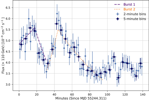
Figure 2. Light curve (2 and 5 minute bins) for VERITAS Mrk 421 data above 110 GeV for the first 2.33 hr of observations on MJD 55244, where two “bursts” are identified via a Bayesian block analysis. The dashed lines show an exponential (Exp) function fit to the rise and fall of the two bursts using the 2 minute binned light curve. The fit parameters, including the rise and decay times, are provided in Table 1. The data behind this figure and Figure 3 are available in FITS format. The first extension provides the 2 minute binned data, while the second gives the 5 minute binned data.(The data used to create this figure are available.)
Download figure:
Standard image High-resolution imageFigure 1 shows the full set of VHE data during 2010 February binned in nightly bins. The first observations by VERITAS on 2010 February 17 are likely to have been taken after the onset of the flare; thus, we cannot make any statement about the rise time of the main flare. A decay function ( , where
  is the halving time) was fit to the four VERITAS data points in Figure 1, resulting in a halving timescale of ∼1 day. We fit the same function to the 10 minute binned data, resulting in a halving time of 1.17 ± 0.07 days, consistent with the nightly binned result.
A Bayesian block analysis (Scargle et al. 2013) was applied to the >110 GeV VERITAS data from the flare night to look for any significant change points. Two peaks, or “microbursts,” were identified in this manner in the first ∼140 minutes. Figure 2 shows a zoom-in on this region with the peaks clearly visible in the first ∼95 minutes. Burst 2 shows an apparent asymmetry that can be quantified via the method used in Abdo et al. (2010); the symmetry parameter is found to be ξ = 0.50 ± 0.09, corresponding to moderate asymmetry. We do not quote the asymmetry value for burst 1, as we cannot be certain we observed the full rise of the burst. In addition, we fit several functions to these data to determine the most likely rise and decay timescales for the peaks. We test an Exponential (Exp), ![$F(t)=A\cdot \exp \left[| t-{t}_{\mathrm{peak}}| /{t}_{\mathrm{rise},\mathrm{decay}}\right]$](https://content.cld.iop.org/journals/0004-637X/890/2/97/revision1/apjab6612ieqn6.gif) , and the generalized Gaussian (GG) burst profile from Norris et al. (1996) of the form
, and the generalized Gaussian (GG) burst profile from Norris et al. (1996) of the form ![$F(t)=A\cdot \exp {\left[| t-{t}_{\mathrm{peak}}| /{t}_{\mathrm{rise},\mathrm{decay}}\right]}^{\kappa }$](https://content.cld.iop.org/journals/0004-637X/890/2/97/revision1/apjab6612ieqn7.gif) . The most likely values and uncertainty of the parameters are determined using a Markov Chain Monte Carlo method with the emcee tool (Foreman-Mackey et al. 2013). The most likely values are taken as the 50th percentiles, while the uncertainties are given as 90% confidence intervals of the posterior distributions of the parameters. The fit results are provided in Table 1. For burst 2, the GG profile with one more parameter than the Exponential function is not statistically preferred. In Section 5 we use the burst 2 rise time, trise = 22 minutes, to place an upper bound on the effective size of the emission region, as well as a lower bound on the Doppler factor when taking into account the compactness and opacity requirements of the emitting region.
. The most likely values and uncertainty of the parameters are determined using a Markov Chain Monte Carlo method with the emcee tool (Foreman-Mackey et al. 2013). The most likely values are taken as the 50th percentiles, while the uncertainties are given as 90% confidence intervals of the posterior distributions of the parameters. The fit results are provided in Table 1. For burst 2, the GG profile with one more parameter than the Exponential function is not statistically preferred. In Section 5 we use the burst 2 rise time, trise = 22 minutes, to place an upper bound on the effective size of the emission region, as well as a lower bound on the Doppler factor when taking into account the compactness and opacity requirements of the emitting region.
Table 1. Results from Fits to the 2 Minute Light Curves for the Two Bursts Shown in Figure 2
| Burst | Fit | A | trise | tdecay | tpeak | κ | χ2/NDF |
|---|---|---|---|---|---|---|---|
| Function | (minutes) | (minutes) | (minutes) | ||||
| 1 | Exp | 5.5+0.34−0.28 | 84+∞−49 |

|

|
⋯ | 18/12 |
| GG |

|

|

|

|

|
11/11 | |
| 2 | Exp |

|

|

|

|
⋯ | 30/29 |
| GG |

|

|

|

|

|
27/28 | |
Note. The quoted (most likely) values represent the 50th percentile, while the uncertainties are given as the 90th percentile of the posterior distributions of the parameters. Here trise and tdecay are the doubling and halving timescales, respectively. The units for the normalization A are [10−9 photons cm−2 s−1 TeV−1]; κ is unitless.
Download table as: ASCIITypeset image
3.2. Search for VHE Hysteresis during Flare
In order to investigate possible relationships between flux and photon index for the >110 GeV VERITAS data, coarser 5 minute bins were used for reducing statistical uncertainties. Within each time bin, a flux estimation and full spectral reconstruction were performed. The Mrk 421 spectra are curved within each 5 minute bin; therefore, an exponential cutoff power-law function,

was used to reconstruct and fit the spectra, where Ecut is the cutoff energy. The Ecut parameter was kept fixed to Ecut = 4 TeV, the value from a global fit. Figure 3 displays the resulting photon index versus flux representation of the VERITAS detections of Mrk 421 for the two identified bursts. While there is some evidence for a counterclockwise hysteresis loop or a softer-when-brighter trend for burst 1, the photon index in burst 2 is very stable while the flux rises and falls by a factor of ∼1.5.
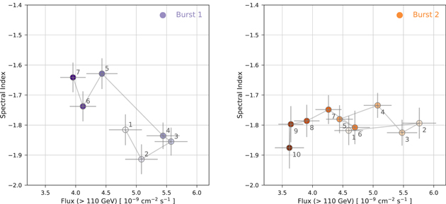
Figure 3. Photon index vs. flux of the VERITAS detections of Mrk 421 over 5 minute intervals shown separately for bursts 1 (left) and 2 (right). The colors represent the chronological progression of the bursts, with lighter colors corresponding to earlier times. The indices are obtained by a fit with an exponential cutoff power law (Ecut), where Ecut is fixed to the global value of 4 TeV. The data behind this figure and Figure 2 are available in FITS format.(The data used to create this figure are available.)
Download figure:
Standard image High-resolution imageThe index–flux relationship for burst 1 was assessed with simple χ2 tests using the observed quantities against constant and linear models as the null hypotheses. A constant model can be rejected with a p-value of 3.2 × 10⁻⁵ (χ2/NDF = 30/6), while the p-value for a linear model is 0.07 (χ2/NDF = 10/5). A χ2 difference test prefers the linear model over the constant model with a p-value of 6.8 × 10⁻⁶. To test the statistical robustness of this relationship, the observed data points were resampled within the measurement uncertainties, and the χ2 tests were repeated for 100,000 iterations. At a 90% confidence level, the constant model is rejected 99.7% of the time, while the linear model is rejected 81.9% of the time. The p-value for the linear model indicates that the index–flux relationship for burst 1 appears only marginally consistent with a linear (softer-when-brighter) trend. The deviation from a linear trend could be an indication of a more complicated relationship between the Mrk 421 index and flux, such as a hysteresis loop.
These index–flux characteristics, along with the asymmetry of burst 2, can be used to infer differing relationships between the cooling and acceleration timescales for the bursts, which is further discussed in Section 5.
3.3. VHE γ-Ray and Optical Correlation Studies
The RCT R-band optical data are the only data set other than VERITAS to have high statistical sampling during the night of the VHE highest state (MJD 55244). Figure 4 shows the VERITAS 2 minute binned data (blue) over the full energy range (420 GeV < E < 30 TeV) commensurate with the low-elevation threshold, and the R-band optical data (orange) are overlaid. Visual inspection indicates an apparent correlation between the two wave bands, which warrants further investigation.
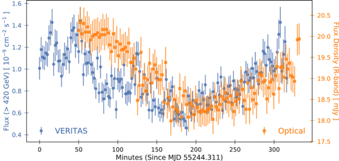
Figure 4. The 2 minute binned VERITAS >420 GeV (blue) and RCT optical R-band (orange) light curves during MJD 55244. The data behind this figure are available in FITS format. The first extension provides the VERITAS data, while the second gives the RCT R-band photometry.(The data used to create this figure are available.)
Download figure:
Standard image High-resolution imageWe used the discrete cross-correlation function (DCCF) analysis following Edelson et al. (1990) to test for time lags between the 2 minute binned VERITAS and RCT light curves. The DCCF was calculated after subtracting the mean from each light curve and dividing the result by the standard deviation. There is a broad peak apparent in the DCCF (turquoise points in Figure 5) centered at a lag time of roughly 45 minutes, with VHE γ-rays leading the optical.
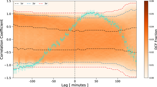
Figure 5. Simulated DCCFs for VERITAS (>420 GeV) and optical R-band light curves. The DCCF from observations is in turquoise. Here “DCF fraction” represents the fraction of times a simulated DCCF falls in a given lag-time and correlation-coefficient bin (shown with the 2D histogram color map). The DCF fraction histogram (representing a PDF) is integrated to obtain the confidence levels. The black, blue, and red dashed lines show the 1σ, 2σ, and 3σ levels, respectively. A positive lag time corresponds to a delay in the optical light curve with respect to the VERITAS light curve.
Download figure:
Standard image High-resolution imageIn order to assess the statistical significance of features in the DCCF, including the broad peak, Monte Carlo simulations were performed following the method by Emmanoulopoulos et al. (2013). First, as described in Appendix A, the PSD was constructed and fitted for both the VERITAS and optical light curves. Next, the best-fit VERITAS PSD (P(f) ∝ f−1.75) was used to generate 100,000 random light curves. The random light curves were then paired with the observed optical light curve to calculate a DCCF for each iteration.
Figure 5 shows the resulting simulated DCCFs binned into a 2D histogram of correlation-coefficient versus lag-time bins. The bin contents of the 2D histogram are normalized such that for a fixed lag time, each correlation-coefficient bin gives the fraction of all DCCFs falling within the bin, and the bin contents along the vertical axis will sum to 1. Significance levels are estimated by integrating the probability density function (PDF) represented by the 2D histogram of simulated DCCFs. The VERITAS–optical DCCF shows evidence for a signal at lag times of 25–55 minutes. The significance of the correlation is ∼3σ. The use of an observed light curve (in this case, the optical R band) in the significance level estimation is a conservative approach. If simulated light curves are generated from the optical PSD (P(f) ∝ f−1.85), the correlation significance increases to ∼4σ. We note, however, that the PSD fit errors are large, hindering a good characterization of the uncertainties on the significance of the correlation.
3.4. Autocorrelation Analysis with the VHE Flare
The VHE flux from Mrk 421 shows clear intranight variability during the night of the flare on 2010 February 17, and the PSD analysis for VERITAS from Appendix A shows a power spectrum of pink noise (or flicker noise) with P(f) ∝ f−1.75. However, these results are limited to shortest timescales of ∼500 s.
A modified autocorrelation function (MACF) proposed in Li (2001) and extended in Li et al. (2004) could provide improved sensitivity to short variations of the VHE flux. Details of the method can be found in Appendix B. Though Bolmont et al. (2009) used the method to search for signatures of potential Lorentz invariance violation in the 2006 PKS 2155–304 flare, it is a novel technique for VHE variability studies. In Appendix B, we have applied the MACF to the night of the VHE flare (epoch 3; see Section 4.1) using all events above an energy threshold E = 420 GeV. No critical timescale is observed on these short timescales, but the data are consistent with a stochastic process or “pink noise” corroborating the VERITAS PSD results found at longer timescales in Appendix A. Probed by the combination of these two techniques, this is the first time that this stochastic behavior has been shown to exist in a blazar on the full range of timescales from seconds to hours.
4. Results from Full 2010 February Multiwavelength Data Set
4.1. Light Curves
In this section, we focus on the multiwavelength light curves of Mrk 421 for 2010 February. Figure 1 shows the light curves for each wave band participating in the campaign. The VHE data are shown averaged over the full set of observations for a given night spanning durations between ∼20 minutes and ∼6 hr, Fermi-LAT and MAXI data are shown with daily binning, and all other light curves are binned by individual exposures. To study the flux properties of the VHE data in more detail, the entire combined MAGIC and VERITAS data set from Figure 1 was split into multiple epochs. MAGIC data are available for several days leading up to the flare. These epoch 1 data (MJD 55232–55240) are used as “baseline” VHE data to which we compare the flaring period and its decline. Epoch 2 (MJD 55240–55243) has no VHE data; however, it is used to study the behavior of the X-ray and HE data as the flare builds up in these bands (see Section 4.4). Epoch 3 comprises the main flare (MJD 55244) showing extraordinary overlap between the VHE and optical data enabling the correlation analysis shown in Section 3.3. Epochs 3–7 (MJD 55244, 55245, 55246, 55247, and 55248) are shown in Figure 6, which displays 10 minute binned light curves for both VHE and RXTE X-ray data (top panel). Epochs 3–6 comprise only VERITAS data in the VHE band (shown above 350 GeV as the lowest common threshold) and are, respectively, during the VHE flare and just afterward in three decline epochs. Epochs 4–7 comprise RXTE data in the 3–15 keV band where epochs 3–6 overlap with the VERITAS data during the decline phases, and a subsequent rise in RXTE data is seen in epoch 7; no VHE data are available in this last epoch. During periods where strictly simultaneous data were obtained, we matched the start and stop times of each time bin between the VERITAS and RXTE light curves. These VHE and X-ray light curves, along with the VERITAS photon indices and RXTE hardness ratios shown in the bottom panel of Figure 6, are used in more detailed studies in Section 4.3. However, first we compare variability properties across all participating wave bands shown in Figure 1.
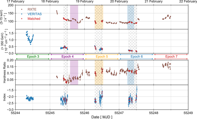
Figure 6. Detailed 10 minute binned light curves for VHE (VERITAS; blue) and X-ray (RXTE; brown) data for epochs 3–7: the VHE flare (epoch 3) followed by the three VHE decline epochs (epochs 4–6) and a final epoch during which RXTE count rates are elevated again. Matched, shown by red points, distinguishes data where there is strictly simultaneous overlap between RXTE and VERITAS observations. The top panel shows the RXTE count rate and VERITAS flux light curves as a function of time, while the bottom panel shows the RXTE hardness ratio between the 5–15 and 3–5 keV bands and the VERITAS photon index from power-law fits between 350 GeV and 3 TeV. We note that there are no simultaneous X-ray data during the VHE flare (epoch 3), and there are no VHE data during epoch 7. Regions of overlap are indicated by gray hatches, and their behavior is studied in Section 4.3. Colored shaded regions are used for a more in-depth X-ray hardness ratio–count rate study illustrated by the bottom panels of Figure 13. The data behind this figure are available in FITS format. The first extension provides the RXTE data, while the second gives the VERITAS data.(The data used to create this figure are available.)
Download figure:
Standard image High-resolution image4.2. Multiwavelength Variability
We calculated the fractional rms variability amplitude Fvar (Edelson et al. 1990; Rodríguez-Pascual et al. 1997)—as defined by Equation (10) in Vaughan et al. (2003), with its uncertainty given by Equation (7) in Poutanen et al. (2008)—for each available band, with the results shown in Figure 7. The Fvar calculation was performed for the full duration of the light curves shown in Figure 1 and separately for the 2 minute binned optical and VERITAS (three bands) light curves from the night of the giant flare (MJD 55244). Note that the four radio bands are shown under a single point covering the energy range of the bands, as no excess variance (Fvar = 0) was found in any of the bands.
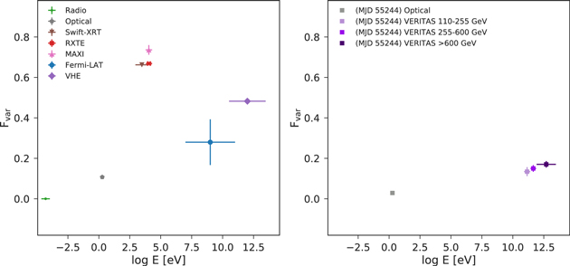
Figure 7. Left: fractional variability for each wave band over the full data set shown in Figure 1 (key in top left corner). The VHE band uses the nightly averaged binning from Figure 1 for both the VERITAS and the MAGIC light curves; the optical and radio bands include observations from all participating observatories displayed in Figure 1. Right: Fvar calculated for the 2 minute binned light curves produced for the optical and three separate VERITAS energy bands on the night of the main flare, as shown in Figure 4 (key in top left corner).
Download figure:
Standard image High-resolution imageThe Fvar values from the full light curves spanning the month of 2010 February increase from radio to optical to X-ray, drop again for the HE band, and then show maximal Fvar for the VHE band. This “double-humped” Fvar characterization, which has been observed in Mrk 421 during low and high activity (Aleksić et al. 2015a, 2015b; Baloković et al. 2016), could reflect the global difference in cooling time between the populations of electrons underlying the different bands. However, no strong conclusions can be drawn from these values, as the integration times differ drastically for the light curves from different instruments, potentially introducing large biases.
The Fvar values for the optical and VERITAS light curves from MJD 55244 are more reliable for interband comparison, showing higher values for the VERITAS bands compared to the optical and an indication of an increasing trend with energy within the three VERITAS bands (though the p-value of a χ2 difference test between a linear and constant fit is 0.13). If the particle-cooling timescale (with IC scattering or SSC) is longer than the dynamical timescale of the emission region, the increasing Fvar with energy observed in the VHE can be related to the difference in cooling times between particles of different energies. The higher-energy particles will cool faster, producing larger variability and a correspondingly higher Fvar value for a given timescale than lower-energy particles that cool more slowly.
There is a large contrast between the impressive flux variations at high energies and the muted behavior in both optical flux and linear polarization seen in Figure 1. The optical data show a smooth decrease of 20% over the entire period. Two “fast” variations (1–2 day timescales) of about 15%–20% are noted: one on MJD 55236 (2010 February 8) in epoch 1 in the “preflare” time interval and the other in epoch 2 on MJD 55244 (2010 February 16), the night before the ∼11 CU (above 110 GeV) flare measured with VERITAS. This latter fast optical variation is during the period where the HE and X-ray observations show some evidence for correlation (see Section 4.4). It is interesting to note that, while the source clearly stayed high on 2010 February 17 in X-rays and VHE, the optical flux diminished to values just slightly higher than the pre-/postflare flux.
The optical polarization for Mrk 421 increased from P = 1.7% to 3.5% during the VHE flare. No change in polarization position angle was detected over the same period, although larger (∼20°) position angle swings are observed just prior to and after the VHE flare. In general, both the variability in optical flux and polarization are mild during this period, with P = 1%–3.5% and θ = 125°–155°. For comparison, the Steward Observatory monitoring data for Mrk 421 obtained during the 2010 January and March observing campaigns show the blazar to be more highly polarized. For 2010 January 14–17, P = 3.7%–5.0% and θ = 157°–163°, and during 2010 March 15–21, P = 3.1%–4.9% with θ = 114°–130°. In addition, the object was about 0.3 mag brighter during the 2010 January campaign compared to the February measurements, while it was <0.1 mag fainter in 2010 March.
There are no signs of unusual activity in the radio observations of Mrk 421 with the instruments that participated in this campaign (UMRAO, Metsähovi, and OVRO) over the 2 weeks before and 2 weeks after the main VHE flare. However, no observations were taken during the VHE flare night. High-resolution Very Long Baseline Array (VLBA) observations of Mrk 421 were collected on 2010 February 11 as part of the Monitoring Of Jets in Active galactic nuclei with VLBA Experiments (MOJAVE) program (Lister et al. 2018). MOJAVE data on Mrk 421 are also available from 2009 December 17 and 2010 July 12 observations. The 15 GHz MOJAVE images show significant extended structures associated with the source. The emergence of a potentially new component within the Mrk 421 milliarcsecond radio jet over the month following the giant flare was reported by Niinuma et al. (2012) using the Japanese Very Long Baseline Interferometry (VLBI) Network and Jorstad et al. (2017) using observations from the VLBA blazar program from Boston University. However, we cannot conclude that any of the components from MOJAVE or the VLBI observations are associated with the 2010 February 17 VHE flare. The relative VLBA flux density, SVLBA/Stotal (Stotal is the filled-aperture single-antenna flux density) from the 2010 February 11 MOJAVE and 2010 February 12 OVRO observations is comparable to the average historical value of ∼0.75 from Kovalev et al. (2005). The parsec-scale jet direction reported in Jorstad et al. (2017) is about −25°, and the polarization angle of the radio knot B1 is about −35°, both angles being approximately the same as those reported in Figure 1 for the optical electric vector polarization angle (EVPA), taking into account the ambiguity of the EVPA with respect to π.
4.3. VHE γ-Ray and X-Ray Correlation Studies
By visual inspection of Figure 1, we cannot ascertain whether the VHE flare was observed at its peak or on the decline. Furthermore, there are no overlapping Swift-XRT or RXTE data during the night of the highest VHE flux. Unfortunately, we therefore cannot determine any correlation between X-ray and VHE at the peak observed in either band. There are only three Swift-XRT exposures over the first 2 days of the decline, averaging 3.6 ks per exposure. Kapanadze et al. (2018) analyzed these data along with all available Swift-XRT data for the period 2009–2012. However, the RXTE data comprise eight short (average 3.6 ks) and five long (from 9.8 to 48.2 ks) observations during the decline epochs 4–6, which overlap with VERITAS data. We thus use the RXTE data for our in-depth VHE–X-ray studies; both of these data sets are shown in Figure 6, with a zoomed-in version overplotting RXTE and VERITAS data for epochs 4–6 in the top three panels of Figure 8. Clear interday variability is evident in both the VHE and X-ray bands, with epoch 4 mainly comprising a strong decay in an X-ray flare (40% drop in PCA rate), while the VHE shows a slight rising trend, epoch 5 catches the tail of another smaller X-ray flare followed by a rise (both mirrored in the VHE), and epoch 6 shows minimal X-ray and VHE variability.
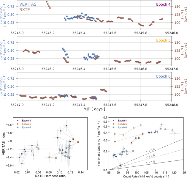
Figure 8. Top three panels: detailed 10 minute binned light curves for epochs 4–6 from Figure 13 with VHE (VERITAS; blue) and X-ray (RXTE; brown) overplotted in the same panel to better highlight the trends described in the text. From top to bottom, the panels are epochs 4, 5, and 6. Bottom two panels: VERITAS photon indices vs. RXTE hardness ratios (left) and VERITAS and RXTE flux–flux correlation plots (right) based on the 10 minute binned light curves for each of the epochs in the above panels. Here we only plot points that correspond to the “matched” points in Figure 6 where there is strictly simultaneous overlap between RXTE and VERITAS observations. Gray lines and color gradients are intended to guide the chronological progression of the points. The hardness ratio is taken between the 5–15 and 3–5 keV bands, while the VHE indices are found from a power-law fit between 350 GeV and 3 TeV.
Download figure:
Standard image High-resolution imageIn Figure 6, we also show the VERITAS photon indices, as well as the RXTE hardness ratio, in 10 minute time bins (bottom two panels). The hardness ratio is taken between the 5–15 and 3–5 keV bands, while the VHE indices are found from a power-law fit between 350 GeV and 3 TeV. Here we note that the overall trend for the X-ray data is an increase in the hardness ratio, while the source in general is becoming steadily weaker in the X-ray (top panel of Figure 6). On the other hand, the VHE data show no general trend during the decline phases of the flaring period. However, there are periods when the VHE indices become significantly harder than Γ ∼ −2, indicating that the VHE emission is in part below the IC peak frequency. Some of these exceptionally hard indices correspond to instances in which the VHE flux is at its weakest in this data set. This is especially true toward the end of Epoch 6.
The bottom left panel of Figure 8 looks at the VHE index versus X-ray hardness ratio over the full decline phase but restricted to data pairs where there is an exact time match between the VERITAS and RXTE data (gray bands in Figure 6). The data suggest a clustering around distinct states that represent “snapshots” of the evolving system over several days. The cluster of extremely hard VHE indices and high X-ray hardness ratio values corresponds to a weak flux state observed in both bands. Though unusual, these observations could indicate both the synchrotron and IC peaks shifting together to higher frequencies (without an increase in peak luminosity).
As there are substantially more X-ray data than VHE data throughout the decline epochs, in Appendix C we carry out a detailed examination of the X-ray data, searching for evidence of hysteresis in the relationship between hardness ratio and count rate. All epochs show a considerably different evolution of the hardness ratio with flux, with a variety of loops and trends exhibited even as an overall increase in hardness ratio is seen as the source weakens in the X-ray across the decline (as noted in Figure 6). The standard harder-when-brighter scenario is only distinctly observed in epoch 5.
To further investigate the flux–flux relationship between the synchrotron and IC peaks during epochs 4–6, we show the VHE–X-ray flux–flux plot in the bottom right panel of Figure 8 for each epoch, where the X-ray and VHE data are simultaneous (indicated by the gray bands in Figure 6). We also show the linear, quadratic, and cubic slopes corresponding to the relation  , with fit values shown for each epoch displayed in Table 2, along with the slopes for subsamples of the data in each epoch and the full data set. For simple SSC behavior, we would expect to see a correlation between the X-ray and VHE emission with a linear correlation slope indicating that the system was in the Klein–Nishina (KN) regime (Tavecchio et al. 1998). In fact, the VHE–X-ray flux–flux plot shows inconsistent behavior across the three epochs. When considering the first four points, epoch 4 shows a hint of an anticorrelation between the VHE and X-ray bands, which would be very inconsistent with a single-zone SSC model. Taking the last six points of epoch 4, no correlation is seen; the VHE stays roughly constant in flux as the X-ray dims. Epoch 5 captures a fast decrease in both VHE and X-ray, followed by a less dramatic rise in both bands. Both the fall and rise states show a correlation between the two bands; however, with ∼quadratic behavior in both “cooling” and “acceleration,” epoch 6 shows an erratic, uncorrelated relationship in time between the X-ray and VHE bands, though with a global fit nearly quadratic in slope. Taken together, the range of behavior across the decline epochs between and within the X-ray and VHE bands is difficult to interpret as the evolution of the system in the context of a single-zone SSC model.
Table 2.
Results from Fits to the Data for the Left Panel of Figure 8 with the Relation 
| Data Set | Γ |
 /NDF /NDF |
ρ | p-value |
|---|---|---|---|---|
| Full | 3.3 ± 0.2 | 220/30 | 0.76 | 3.6 × 10⁻⁷ |
| Epoch 4 (all) | 1.5 ± 0.07 | 16/8 | 0.22 | 0.52 |
| Epoch 4 (first 4) | −1.6 ± 0.18 | 0.85/2 | −0.86 | 0.14 |
| Epoch 4 (first 5) | −3.2 ± 1.2 | 5.4/3 | −0.78 | 0.17 |
| Epoch 4 (last 6) | 0.7 ± 0.09 | 0.34/4 | 0.57 | 0.24 |
| Epoch 5 (all) | 2.0 ± 1.0 | 37/7 | 0.35 | 0.36 |
| Epoch 5 (first 4) | 2.5 ± 0.8 | 1.5/2 | 0.92 | 0.078 |
| Epoch 5 (last 5) | 1.6 ± 1.0 | 1.3/3 | 0.74 | 0.15 |
| Epoch 6 (all) | 1.9 ± 0.1 | 6.9/11 | 0.48 | 0.095 |
| Epoch 6 (no last point) | 1.6 ± 0.3 | 2.1/10 | 0.64 | 0.024 |
Note. Here Fγ is the VERITAS flux above 350 GeV in units of 10−9 cm−2 s−1, FX is the RXTE count rate between 3 and 15 keV, and Γ is the index. The Pearson’s ρ is shown along with the p-value for each fit.
Download table as: ASCIITypeset image
4.4. HE γ-Ray and X-Ray Correlation Studies
By inspection of the light curve in Figure 1, epoch 2 shows an increase in both the MAXI X-ray and Fermi-LAT HE γ-ray daily binned fluxes the day prior to the VHE flare observed with VERITAS. A simple test for variability was performed on the Fermi-LAT light curve. This yielded an improvement in log-likelihood over a constant model equivalent to χ2 = 39.2 for 23 degrees of freedom, corresponding to a p-value of 0.018. The MAXI light curve is clearly variable (χ2/NDF = 930/23; p-value ∼ 0).
A preliminary cross-correlation analysis using Fermi-LAT “Pass7” P7SOURCE_V6 event selection and instrument response functions found that the lag between the X-ray and HE γ-ray light curves was consistent with zero days (Madejski et al. 2012). We performed an analysis using the “Pass8” Fermi-LAT data and instrument response functions corresponding to those used to generate the Fermi-LAT light curve in Figure 1. A linear correlation coefficient was calculated for the time-matched MAXI and Fermi-LAT fluxes, resulting in a mean value of ρ = 0.54 ± 0.12. The mean value and 1σ uncertainties of the linear correlation coefficient were determined by resampling both light curves within measurement uncertainties over 100,000 iterations.
To further investigate this potential correlation, we conducted a DCCF analysis between MAXI–Fermi-LAT light curves in the manner described in Section 3.3. In this case, the PSD from the MAXI light curve was fit using the method by Max-Moerbeck et al. (2014), and the best-fit MAXI PSD (P(f) ∝ f−1.95) was used to generate 100,000 random light curves paired with the observed Fermi-LAT light curve (the conservative approach), with the results shown in Figure 9.
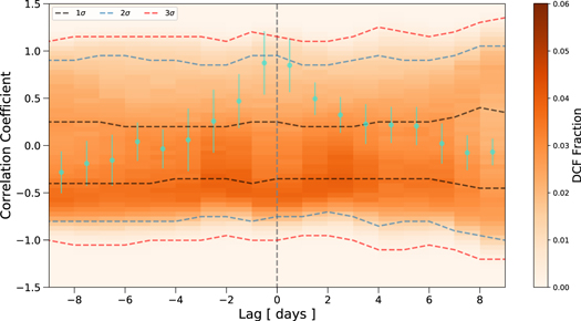
Figure 9. The DCCF calculated from the observed MAXI–Fermi-LAT light curves is shown with turquoise points. Correlation significance levels (shown with dashed lines) are estimated through a Monte Carlo method. During each iteration, the observed Fermi-LAT light curve is paired with a light curve simulated from the MAXI PSD to calculate a simulated DCCF. Here “DCF fraction” represents the fraction of times a simulated DCCF falls in a given lag-time and correlation-coefficient bin (shown with the 2D histogram color map). The DCF fraction histogram (representing a PDF) is integrated to obtain the confidence levels.
Download figure:
Standard image High-resolution imageWe find an ∼2σ correlation at a lag of ∼zero days. The confidence level of the correlation at ∼zero days is considerably higher (∼4σ) if the light curves are simulated from PSDs for Fermi-LAT as well (with the best-fit PSD P(f) ∝ f−1.75). The PSD fit errors are very large, however, making it difficult to characterize the uncertainties on the significance of the correlation.
5. Discussion and Conclusions
The VHE flare observed from Mrk 421 in 2010 February is a historically significant flare. During the night of the giant flare observed with VERITAS, Mrk 421 reached a peak flux of about 27 CU above 1 TeV. This episode rivals the brightest flares observed from any source in VHE γ-rays, including the extraordinary flare of PKS 2155–204 in 2006 detected by H.E.S.S. (Aharonian et al. 2009) and the 2001 February 27 flare of Mrk 421 seen with Whipple (Krennrich et al. 2001; Acciari et al. 2014). Another exceptionally strong flare in Mrk 421 was detected by both VERITAS and MAGIC in 2013 April (Cortina & Holder 2013). As extreme as the currently reported flare is, it is unclear from the analyses described in this paper and summarized below whether this represents a fundamentally different behavior state for this object or just an extreme end of the same underlying processes that have yielded the range of behavior previously reported.
5.1. VHE–Optical Band Correlation
A cross-correlation analysis was performed between the VHE and optical bands during the night of the VHE flare. The observed optical and VERITAS 2 minute binned light curves exhibit a 3σ–4σ significance correlation with an optical lag of 25–55 minutes centered at 45 minutes. Such behavior can be accommodated under a single-zone SSC scenario, in which the emission in both the VHE and optical bands is produced by a single distribution of electrons. Under this scenario, the optical lag could be explained by the slower cooling of the less energetic electrons that underlie the optical data compared to the electrons responsible for the VHE emission (Boettcher 2019). The lag timescales can be used to set an additional constraint on the magnetic field strength for future SED modeling efforts.
The VHE–optical correlation has been previously observed in HBLs, but not with a lag or at the short timescales probed by this unprecedented data set. For example, the 2008 multiwavelength campaign on PKS 2155–304 reports a >3σ correlation between the H.E.S.S. data and the V, B, and R optical bands on daily timescales and with no lag (Aharonian et al. 2009). It is more common to observe a correlation between the HE and optical, which is likely explained by both bands arising from the same electron population in the simple SSC model (Cohen et al. 2014).
5.2. Fast Variability in VHE γ-Rays
The exceptional brightness of the flare on 2010 February 17 in VHE enabled VERITAS to produce 2 minute binned light curves with 10σ significance in each bin yielding strongly detected, short-term variability. The variable emission within the first 95 minutes of VERITAS observations on that night can be described by at least two successive bursts. Burst 2 is characterized by an asymmetric profile with a faster rise time followed by a slower decay. This behavior has been previously observed (e.g., Zhu et al. 2018) and is typically attributed to emission from electrons with longer cooling than the dynamical timescales, assuming both the cooling and dynamical timescales are much longer than the acceleration timescale. Under this scenario, the flare rise time is related to the size of the emission region (e.g., Zhang et al. 2002).
Assuming the above conditions, we used the rise timescale of burst 2 to place an upper limit on the size of the emission region associated with the burst, RB,

where c is the speed of light, tvar is the variability timescale, and δ is the Doppler factor. Using the most likely burst 2 rise time of 22 minutes for tvar, we obtained  cm.
cm.
Furthermore, the time variability of the VHE flux, in conjunction with the compactness and opacity requirements of the emitting region, can be used to give an estimate of the minimum Doppler factor of the ejected plasma in the jet of the blazar. Following Dondi & Ghisellini (1995) and Tavecchio et al. (1998) the minimum Doppler factor was calculated using

where σT is the Thomson scattering cross section, dL is the luminosity distance of the source, z is the redshift, tvar is the observed variability timescale, and F(ν0) and β are the flux and spectral index, respectively, of the target photons of the γ-rays for pair production.
To estimate the Doppler factor limit, we used the following parameters: the observed variability timescale tvar,VHE = 22 minutes; the γ-ray photon energy Eγ = 110 GeV, corresponding to a target photon frequency of 6.0 × 10¹⁴ Hz (500 nm) for a maximum pair-production cross section; and the spectral index, β = −0.16, and F(ν0) = 1.35 mJy of the low-energy photons derived from the three Swift-UVOT-band observations during MJD 55244–55246. The latter value was obtained using  . Assuming these parameters, the derived Doppler factor lower bound is δmin ≳ 33. The fast variability measured with this data set results in a larger Doppler factor compared to Błażejowski et al. (2005), where a lower limit on the Doppler factor of δmin ≳ 10 was obtained with an ∼hour-scale time variability in the VHE data from the 3 CU flare of Mrk 421 during 2004 April.
For the overall system to be consistent with reported lower Doppler factors from VLBI measurements, results from fast flares such as that reported here indicate that the γ-ray emission zone may be smaller than the jet cross section. For example, Giannios (2013) suggested that rapid ∼minute-scale flares on an “envelope” of day-scale flares can be due to large plasmoids created during a magnetic reconnection event. However, Morris et al. (2018) showed that while such a “merging plasmoid” model can explain the VHE light curve from the 2016 fast flare from BL Lac (Abeysekara et al. 2018), it has difficulty reproducing the SED.
A potential counterclockwise loop (known as spectral hysteresis), or a harder-when-weaker trend, is present in the index versus flux representation for burst 1, while the photon index is essentially constant for burst 2 even as the flux changes by a factor of ∼1.5. Spectral hysteresis can occur as a result of competing acceleration, cooling, and dynamical timescales, which determine how the effects of particle injection into an emitting region translate to the observed photons (Kirk et al. 1998; Li & Kusunose 2000; Böttcher & Chiang 2002). Counterclockwise hysteresis is related to a case in which dynamical, acceleration, and cooling timescales are comparable. The change in the number of emitting particles in this scenario is determined by the acceleration process, which proceeds from lower to higher energies and leads to higher-energy photons lagging behind lower-energy photons.
A modified autocorrelation analysis is applied to the VERITAS data on the night of the flare to look for potential variability on short timescales; however, no significant time structures are found within 10–60 s timescales. Combining this result with timescales probed by the VHE PSD analysis, we conclude that the VHE emission is consistent with a pink-noise characterization over a wide range of timescales from ∼seconds to ∼hours. Power-law PSDs in blazars have been detected in X-rays as well as VHE and are indicative of an underlying stochastic process (Aharonian et al. 2007). A power-law PSD could also point to a self-organizing criticality (SOC) system, such as magnetic reconnection, as the underlying physical process responsible for the flaring behavior observed for Mrk 421 (Lu & Hamilton 1991; Aschwanden 2011; Kastendieck et al. 2011). A recent study of Mrk 421 flares extracted from archival XMM-Newton X-ray data spanning 2000–2017 is consistent with the expectations for an SOC model, thus lending support to the magnetic reconnection process driving blazar flares (Yan et al. 2018). Additionally, the flatness of the PSD indicates that the turn-on/turn-off timescale of mini-flares can be below 1 hr and generally has a wide probability distribution extending from subhour timescales to entire nights (Chen et al. 2016).
5.3. Multiwavelength Correlation Studies
In addition to the optical–VHE correlation study, several other intraband and multiband correlation studies were carried out. The decay of the flare in the VHE and X-ray bands occurs over the course of 4 days. Correlation studies between the VHE (VERITAS) and X-ray (RXTE) bands show a diverse and inconsistent range of behavior across the decline epochs. The flux–flux relationship between the synchrotron peak (as probed by the X-ray data) and the IC peak (as probed by the VHE data) moves in epoch 4 from an indication of anticorrelation to no correlation. Błażejowski et al. (2005) reported a lack of correlation seen in day-scale coincident VHE (Whipple) and X-ray (RXTE) data, which is potentially explained by an X-ray flare leading the VHE flare by 1.5 days. The data set reported in our work indicates a lack of correlation between the X-ray and VHE on the ∼10 minute timescales probing potentially quite different mechanisms. To our knowledge, an anticorrelation between the X-ray and VHE has never before been reported for Mrk 421. Epoch 5 shows ∼quadratic behavior in  , most notably in the “cooling” segment of the epoch. This behavior has been seen before in both Mrk 421 (Fossati et al. 2008) and the exceptional flare in PKS 2155–304 (Aharonian et al. 2009) and is not consistent with the linear relationship expected from a system scattering in the KN regime (Aharonian et al. 2009). However, Thomson scattering into VHE photon energies requires unacceptably large Doppler factors (Katarzyński et al. 2005).
The RXTE results indicate spectral hardening as the source becomes fainter over this period. Such behavior can be an indication of the synchrotron peak shifting to higher frequencies as the flare decays, which would be unusual, or the possibility that the synchrotron photons in the keV band soften first, uncovering a population of harder photons produced in the keV band by the IC process at the beginning of the flare (Li & Kusunose 2000). On the other hand, no clear long-term trends are apparent in the VHE photon index as the flare decays. Nonetheless, it is interesting to note that the VHE indices become harder than −2 at times during the decay period, indicating that the Compton peak moves into the TeV regime even as the overall VHE flux is decreasing. The fact that both the X-ray and VHE data show a harder-when-weaker trend at the same time may indicate that both peaks have shifted and the source has temporarily become an extreme HBL (Costamante et al. 2001; Bonnoli et al. 2015; Cerruti et al. 2015). Time-dependent extreme HBL behavior has recently been reported for Mrk 501 (Ahnen et al. 2018), though it is changing on yearly timescales.
A correlation between the HE and X-ray (MAXI) bands was observed on daily timescales. We found an ∼2σ correlation at a lag of ∼zero days, while a less conservative approach yielded ∼4σ. While unusual, HE and X-ray correlations have been seen in other jetted systems, including NGC 1275, and can indicate, for example, a fresh injection of electrons into the emission region (Fukazawa et al. 2018).
5.4. Multiwavelength Variability
A study of the energy dependence of the fractional variability (Fvar) across all participating instruments resulted in a “double-humped” structure that seems to be characteristic for Mrk 421 in both flaring and quiescent states (Aleksić et al. 2015a, 2015b; Baloković et al. 2016). However, this is quite different from the Fvar characterization seen in the other well-studied nearby HBL, Mrk 501, where a general increase in variability as a function of energy has been observed (Aleksić et al. 2015c; Ahnen et al. 2017, 2018). While a strict comparison is difficult due to the vastly different integration times for the participating instruments in each campaign, the different Fvar dependence on energy between the two sources is likely attributed to the difference in the Fvar values in the X-ray band, with lower X-ray Fvar values typically seen in Mrk 501. This could indicate that the X-ray instruments more often probe the rising edge of the synchrotron peak for Mrk 501 than for Mrk 421, which would be consistent with the synchrotron peak excursions to more extreme HBL regimes seen in Mrk 501 (Nieppola et al. 2006; Ahnen et al. 2018). The upcoming work studying the SEDs constructed from these data can further elucidate these observations.
This research is supported by grants from the U.S. Department of Energy Office of Science, the U.S. National Science Foundation, the Smithsonian Institution, and NSERC in Canada. This research used resources provided by the Open Science Grid, which is supported by the National Science Foundation and the U.S. Department of Energy’s Office of Science, and the National Energy Research Scientific Computing Center (NERSC), a U.S. Department of Energy Office of Science User Facility operated under contract No. DE-AC02-05CH11231. We acknowledge the excellent work of the technical support staff at the Fred Lawrence Whipple Observatory and the collaborating institutions in the construction and operation of the instrument.
The MAGIC collaboration would like to thank the Instituto de Astrofísica de Canarias for the excellent working conditions at the Observatorio del Roque de los Muchachos in La Palma. The financial support of the German BMBF and MPG, the Italian INFN and INAF, the Swiss National Fund SNF, the ERDF under the Spanish MINECO (FPA2015-69818-P, FPA2012-36668, FPA2015-68378-P, FPA2015-69210-C6-2-R, FPA2015-69210-C6-4-R, FPA2015-69210-C6-6-R, AYA2015-71042-P, AYA2016-76012-C3-1-P, ESP2015-71662-C2-2-P, FPA201790566REDC), the Indian Department of Atomic Energy, the Japanese JSPS and MEXT, and the Bulgarian Ministry of Education and Science, National RI Roadmap Project DO1-153/28.08.2018 is gratefully acknowledged. This work was also supported by the Spanish Centro de Excelencia “Severo Ochoa” SEV-2016-0588 and SEV-2015-0548 and Unidad de Excelencia “María de Maeztu” MDM-2014-0369, the Croatian Science Foundation (HrZZ) Project IP-2016-06-9782, the University of Rijeka Project 13.12.1.3.02, the DFG Collaborative Research Centers SFB823/C4 and SFB876/C3, the Polish National Research Centre grant UMO-2016/22/M/ST9/00382, and the Brazilian MCTIC, CNPq, and FAPERJ.
This publication makes use of data obtained at Metsähovi Radio Observatory, operated by Aalto University, Finland, and the OVRO 40 m monitoring program, which is supported in part by NASA grants NNX08AW31G, NNX11A043G, and NNX14AQ89G and NSF grants AST-0808050 and AST-1109911. The UMRAO data were obtained through NSF grant AST 0607523 and NASA Fermi GI award NNX09AU16G. The St. Petersburg University team acknowledges support from Russian RFBR foundation, grant 12-02-00452. The Abastumani Observatory team acknowledges financial support by the Shota Rustaveli National Science Foundation through project FR/577/6-320/13. The Steward Observatory data were obtained under Fermi Guest Investigator Program grant NNX09AU10G. The research at Boston University is supported by NASA grant 80NSSC17K0649 and NSF grant AST-1615796.
Software. VEGAS (Cogan 2008), Event Display (Daniel 2008), MARS (Moralejo et al. 2009), Fermi Science Tools81, HEASoft (FTOOLS+XANADU; HEASARC 2014), REX,85 Xspec (Arnaud 1996), emcee (Foreman-Mackey et al. 2013).
Appendix A: PSDs
For the Mrk 421 VERITAS and optical light curves, PSDs were calculated using the fast Fourier transform method available through the POWSPEC program within the XANADU X-ray astronomical spectral, timing, and imaging software package.86 The PSDs were calculated with both the observed VERITAS and optical light curves, as well as for those where the long-term trends have been modeled and removed. Trend removal was done to avoid potential contamination of higher-frequency signal by lower frequencies. A piecewise continuous linear function—represented by a linear spline with a single node at the best-fit location—was used to model and subtract the long-term trend in each light curve. The observed and detrended light curves are presented in Figure 10. The entirety of both the VERITAS and optical light curves was used. Light curves were split into intervals within which the power spectra were independently calculated and later averaged.
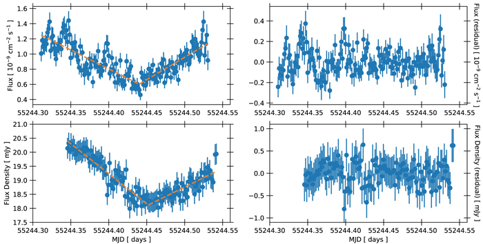
Figure 10. The 2 minute binned VERITAS >420 GeV (top) and optical R-band (bottom) light curves. The left panels are the observed light curves, while the right panels show the light curves after long-term trend removal.
Download figure:
Standard image High-resolution imageThe uncertainties on the power in the individual frequency bins were calculated as the standard deviation of the average of the power from different intervals. The resulting VERITAS and optical PSDs with and without detrending are displayed in Figure 11. The best-fit power-law spectral indices for the VERITAS and optical PSDs were estimated with the method by Max-Moerbeck et al. (2014), resulting in values of −1.75 and −1.85, respectively. The detrended light curves were used to determine whether correlation existed at higher frequencies between the VHE and optical bands; no significant correlation was observed, at least at short timescales.
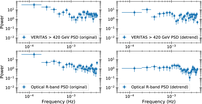
Figure 11. VERITAS >420 GeV (top) and optical R-band (bottom) PSDs with the original observed light curves (left) and light curves after long-term trend removal (right).
Download figure:
Standard image High-resolution imageAppendix B: Modified Autocorrelation Analysis
The modified cross-correlation function (MCCF) is defined as a function of the lag time τ, with τ = kΔt,

where x(t) is the number of counts in the time bin (t, t + Δt), and σ is the standard deviation of x. For this modified correlation function, however, τ is not constrained to be an integer multiple of the light-curve bin size, Δt, and can be incremented by the time-resolution element, δt. The MCCF can then be calculated for lag times, τ = m δt (with m = 0, ± 1, ± 2,…), for light curves with a given timescale Δt. The timescale corresponding to the maximum of MCCF(k δt)/MCCF(0) gives the lag time between x1 and x2.
From the definition of MCCF, the MACF is obtained by setting x1 = x2,

The FWHM of the MACF is a measurement of the variability duration. The maximum of FWHMMACF/Δt may be treated as a characteristic timescale for the time series.
The MACF has the advantage over the regular ACF of being sensitive to variations on timescales smaller than the typical timescales within which significant excess is detected, potentially reaching the time resolution of the instrument  . Thus, the MACF method does not use an ad hoc time binning (for example, the 2 minute bins from Figure 10). Rather, the MACF of the VERITAS flux was constructed assuming a time resolution based on the minimum trigger rate of VERITAS during the Mrk 421 flare observations,
  ms. Then, for a range of ΔT values, where ΔT is some integral number of
  , the correlation was calculated between the initial time series and a new series shifted by the time resolution δt,VER. This “sliding window” process allows the MACF to find any characteristic variability on timescales shorter than the time step ΔT.
Here we have applied the MACF to the night of the VHE flare (epoch 3; see Section 4.1) using all events above an energy threshold E = 420 GeV. Figure 12 shows the FWHMMACF/ΔT as a function of timescale where any characteristic timing signature would show up as a well-defined peak in the data points. The MACFs from simulated events following a pink-noise process (with f−1.75 as above) were also calculated for 1000 iterations and are shown with the color map; they are bounded by dashed red lines at the 99% confidence level.
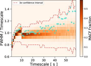
Figure 12. The MACF for the VERITAS events above 420 GeV. Turquoise points show the MACF from VERITAS observations, while the color map bounded by red curves shows the region encompassed by MACFs from events simulated from a pink-noise process.
Download figure:
Standard image High-resolution imageAppendix C: X-Ray Hysteresis Search
We analyzed the RXTE data during the VHE decline (epochs 3–6), calculating the hardness ratio between the 5–15 and 3–5 keV X-ray bands in 10 minute time bins for each of the decline epochs. We then plotted the hardness ratio as a function of counts in the combined 3–15 keV band to look for any evidence of hysteresis. This is shown in the top panels of Figure 13, with a “zoom-in” shown in the bottom panels corresponding to noticeable rise/decline states in the X-ray (indicated by the solid/colored bands in Figure 6). All epochs show considerable evolution of the hardness ratio with flux, with a variety of loops and trends. In particular, the top left panel of Figure 13, with observations from epoch 4, shows an apparent clockwise hysteresis loop between count rates of 100–120 s−1 and hardness ratios of 0.02–0.06. A zoom-in of part of this loop in the bottom left panel of Figure 13 (corresponding to a burst-like feature in the light curve) shows a hardness ratio increase with increasing count rate, followed by a slight, continued increase in hardness ratio as the count rate begins to decrease, and finally a fairly constant hardness ratio even as the count rate decreases significantly.
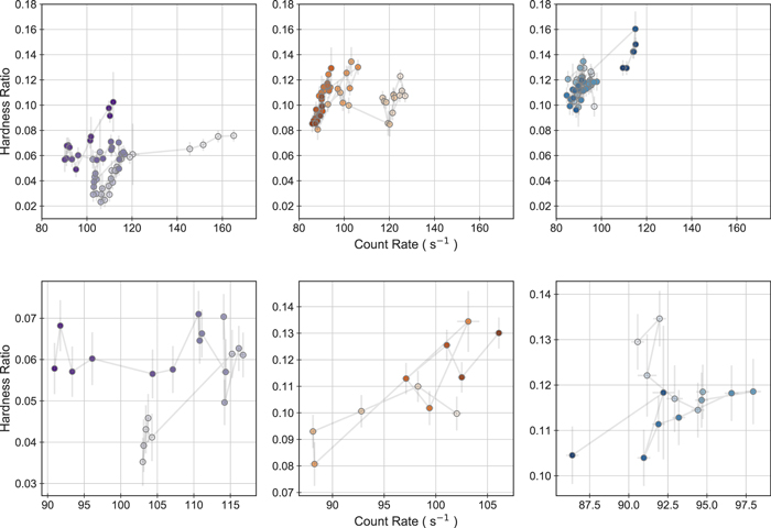
Figure 13. Top panels: hardness ratio (between 5–15 and 3–5 keV) vs. count rate of the RXTE observations of Mrk 421 over the three decline epochs indicated by the arrows in Figure 6 (not strictly simultaneous with VHE data within the epoch). Left: epoch 4; middle: epoch 5; right: epoch 6. The color shading of the data points represents the chronological progression of the bursts, with lighter colors corresponding to earlier times. Bottom panels: zoom-in on hardness ratio vs. count rate of the RXTE observations of Mrk 421 corresponding to the colored bands in Figure 6 (not strictly simultaneous with VHE data within the epoch). Left: epoch 4 zoom-in; middle: epoch 5 zoom-in; right: epoch 6 zoom-in. The color shading of the data points represents the chronological progression of the bursts, with lighter colors corresponding to earlier times.
Download figure:
Standard image High-resolution imageFootnotes
- 81
- 82
- 83
- 84
HEASOFT v6.13, Swift_Rel4.0(Bld29)_14Dec2012, with calibrations from Breeveld et al. (2011).
- 85
- 86