Abstract
It is widely accepted in the MHD turbulence community that the nonlinear cascade of wave energy requires counterpropagating Alfvénic wave packets, along some mean magnetic field. This fact is an obvious outcome of the MHD equations under the assumptions of incompressibility and homogeneity. Despite attempts to relax these assumptions in the context of MHD turbulence, the central idea of turbulence generation persists. However, once the assumptions of incompressiblity and homogeneity break down, the generally accepted picture of turbulent cascade generation is not universal. In this paper, we show that perpendicular inhomogeneities (across the mean magnetic field) lead to propagating wave solutions that are necessarily described by co-propagating Elsässer fields, already in the incompressible case. One simple example of these wave solutions is the surface Alfvén wave on a planar discontinuity across the magnetic field. We show through numerical simulations how the nonlinear self-deformation of these unidirectionally propagating waves leads to a cascade of wave energy across the magnetic field. The existence of this type of unidirectional cascade might have an additional strong effect on the turbulent dissipation rate of dominantly outward-propagating Alfvénic waves in structured plasma, as in the solar corona and solar wind.
1. Introduction
Stemming from the remarkable analogy of the magnetohydrodynamic (MHD) equations to the hydrodynamic equations when expressed in the formalism now bearing his name, Elsässer (1950) was probably the first to point out that “one might, in particular, expect that phenomena of turbulence will occur in hydromagnetic systems. . . . They will no doubt give rise to a ‘turbulent’ magnetic field coupled with the mechanical motion.” Since then, this possibility has been confirmed by numerous direct and indirect observations, for both astrophysical and laboratory plasmas (see, e.g., Tu & Marsch 1995; Bruno & Carbone 2013; Brown & Schaffner 2014). One of the first theoretical breakthroughs toward understanding MHD turbulence was put forth by Iroshnikov (1964) and Kraichnan (1965). They pointed out that the nonlinear, turbulent cascade of energy is the result of collisions (mutual deformation) of oppositely propagating Alfvénic wave packets. This result was based on the assumption of an incompressible and homogeneous plasma. Under these conditions, arbitrarily nonlinear pure Alfvén waves are exact solutions to the MHD equations. In the Elsässer formalism, a pure Alfvén wave is completely described by one of the Elsässer variables,  , with the sign representing parallel (−) or antiparallel (+) propagation, with respect to the mean magnetic field. Nonlinear interactions occur only when both z± are nonzero, thus the need for counterpropagating waves. This central idea is still generally accepted as the basis of MHD turbulence (e.g., Howes & Nielson 2013). For a broader perspective on MHD turbulence, see the review in Zhou et al. (2004). Indeed, it is often not realized that once the assumptions of incompressibility or homogeneity, or both, do not apply, the MHD spectrum is much richer and allows for more complex dynamics than the propagation of pure Alfvén waves (Goossens et al. 2011, 2019). Compressibility allows for the existence of magnetoacoustic waves, which in a homogeneous plasma are the fast and slow waves. Inhomogeneities generally allow for the existence of surface and global waves, which have distinct properties compared to the normal modes of a homogeneous plasma (Priest 2014). MHD waves in an inhomogeneous plasma are also referred to as waves with mixed properties, i.e., both Alfvén and magnetoacoustic properties. The mixed properties arise because in an inhomogeneous plasma the Eulerian perturbation of total pressure couples with the dynamics of the motion (Hasegawa & Uberoi 1982). The linear coupling of the Elsässer variables due to density inhomogeneity (e.g., gravitational stratification in a coronal hole) along the mean magnetic field was shown by Heinemann & Olbert (1980), for an incompressible plasma. This leads to Alfvén wave reflections. The inhomogeneity along the propagation direction acts as a source of inward-propagating Alfvén waves, even if only outward (away from the Sun) propagating waves are present initially. Then, the outgoing and reflected, counterpropagating Alfvén waves lead to turbulence due to the same nonlinear term involving both z± nonzero. Turbulence due to reflected waves is still an intense research topic getting considerable attention (Matthaeus et al. 1999, 2003; Dmitruk et al. 2001; Perez & Chandran 2013; van der Holst et al. 2014; van Ballegooijen & Asgari-Targhi 2016).
However, Velli et al. (1989) and Hollweg (1990) pointed out that linear coupling also implies that modes present both z± nonzero while propagating. The secondary component of z− (say), co-propagating with z+, was referred to as the “anomalous” component. Hollweg (1990) went a step further and stated, based on harmonic analysis, that an Alfvén wave propagating in a plasma that is inhomogeneous along the magnetic field is necessarily described by both  and
and  , and therefore it is “incorrect to make the (common) assumption that an observation of z− (say) represents an outward-propagating Alfvén wave while z+ necessarily represents an inward propagating Alfvén wave.” Velli et al. (1989) proposed that the “anomalous” z− fields are co-propagating with the principal z+ and can lead to a turbulent cascade that is essentially different from that in homogeneous MHD turbulence due to counterpropagating waves. They argued that, as z± are propagating in the same direction with the same velocity, the nonlinear interaction is coherent, modifying the spectral characteristics of the resulting turbulence. The idea of nonlinearly interacting co-propagating z± disturbances was met initially with opposition (Velli et al. 1990; Zhou et al. 1990). Nevertheless, the idea that there are co-propagating z± fields was accepted for nearly two decades, until Hollweg & Isenberg (2007) pointed out that the harmonic analysis in Hollweg (1990) led to wrong conclusions. Using an impulse function approach, Hollweg & Isenberg (2007) show that while the z± fields are indeed coupled for an outward-propagating Alfvén wave, this does not mean that the “anomalous” Elsässer field is co-propagating with the principal one. The leading edge of the “anomalous” component may seem to propagate outward; however, this does not imply that it follows anything other than the inward characteristics in the plasma frame. Hollweg & Isenberg (2007) explain: “A simple analogy might be smoke coming out of the smokestack of a ship that is steaming into a headwind. The front of the smoke trail is always at the forward moving smokestack, but each smoke particle is blown backward by the wind as soon as it leaves the smokestack.” Although this study dismisses the existence of an “anomalous” field that is co-propagating (for the specific setup as in Heinemann & Olbert 1980), it does not change the fact that there can be coherent nonlinear interactions between z±, e.g., at the leading edges of wave packets. What changes is that technically these can still be categorized in the oppositely propagating wave interaction description and do not represent self-deformations of waves. The implications of such coherent nonlinear interactions have since then been exploited in a number of studies (Verdini et al. 2009, 2012). As we will see later, a plasma with density variations (stratification) along the field but otherwise permeated by a straight and uniform magnetic field is a very special case. Under these conditions, one can still globally talk about linearly coupled outward- and inward-propagating pure Alfvén waves. Therefore, it is also a special inhomogeneous setup in which the Elsässer variables still retain their identity, i.e., z+ and z− still represent strictly inward- or outward-propagating Alfvén waves. This peculiarity might be the reason why the existence of truly co-propagating Elsässer fields was missed. In general, the presence of co-propagating Elsässer fields just means that the waves are no longer pure Alfvén waves encountered in a homogeneous plasma. For example, magnetosonic waves in a homogeneous plasma generally present both Elsässer variables while propagating, as do all waves in a generally inhomogeneous plasma (Magyar et al. 2019). Therefore, in this study we shall avoid calling the induced co-propagating Elsässer component “anomalous,” as was customary in the literature. Indeed, there is nothing anomalous in an MHD wave that is not a pure Alfvén wave owing to the presence of inhomogeneities or compression.
Turbulence induced by truly unidirectionally propagating waves proposed in Magyar et al. (2017), which we refer to as “uniturbulence” or self-cascade of waves, is still largely unknown, and it is controversial. This lingering disbelief (since the proposal by Velli et al. 1989) might come from the erroneous conclusion that nonlinear interactions necessarily imply counterpropagating waves, as results from the incompressible and homogeneous MHD equations, or as might result from the setups involving Alfvén wave reflection, described above. Marsch & Tu (1989) and Zhou & Matthaeus (1989) derived the incompressible MHD equations in the Elsässer formalism for a generally inhomogeneous background plasma. These equations show clearly that inhomogeneities act as sources for the z± fields, through which they are linearly coupled. However, this does not necessarily mean only reflection (i.e., creation of counterpropagating waves). It also means that unidirectionally propagating waves are now described by both z± nonzero. Furthermore, in the presence of density inhomogeneities, there are nonzero nonlinear terms involving only either z+ or z−, a deviation from the original Kraichnan (1965) picture. Departure from this picture is also present in homogeneous compressible turbulence, for which the exact relation includes multiple terms without the need for both z± nonzero (Banerjee & Galtier 2013). While inhomogeneities along the magnetic field are a popular initial condition in MHD turbulence studies, there are much fewer studies that deal with inhomogeneities across the magnetic field. Malara et al. (1992) simulated a 2D incompressible plasma with a straight but transversely varying magnetic field. They showed that the initial perturbation consisting of only z+ quickly leads to the generation of z− through the source terms mentioned above. The wave is then phase-mixed (a linear process; Heyvaerts & Priest 1983) in the direction of the inhomogeneity, leading to increasingly oblique wave fronts in time. The authors show (through energy spectra) that nonlinear interactions do occur between z±, but as we will show later, they apparently miss the fact that the generated z− is co-propagating with z+ and attributed it to “waves propagating in opposite directions.” Ghosh et al. (1998) studied a setup with pressure-balanced structures and also showed the generation of z− (say) from a spectrum of pure z+. However, they do not specify the propagation direction of z−, focusing mostly on “refraction of parallel-propagating Alfvén waves to oblique angles,” which is essentially the process of phase mixing.
In this paper, we explore plasmas that are inhomogeneous perpendicularly to a straight magnetic field, both analytically and through numerical simulations. We show that unidirectionally propagating waves lead to nonlinear cascade of energy to higher perpendicular wavenumbers, i.e., they self-cascade. This paper is intended to offer a deeper insight into the phenomenon of uniturbulence and to further bring this new turbulence generation mechanism to the attention of the MHD turbulence community. In Section 2, we start from the incompressible MHD equations to show the wave properties of perpendicularly inhomogeneous plasmas and the peculiarity of the longitudinally inhomogeneous case. In Section 3, we show the results of 3D MHD simulations and the self-cascade of wave energy in a simple inhomogeneous setup. Finally, in Section 4, we provide our conclusions for the presented results.
2. Inhomogeneous Incompressible MHD
We start from the ideal, incompressible MHD equations (e.g., Goedbloed & Poedts 2004):




where  is the current density. Note that the solenoidal condition on the velocity, i.e., incompressibility (∇ · v = 0), is implied by the formulation of the continuity equation in Equation (1). We retain this equation, as we allow for density inhomogeneities. Using the Elsässer variables (Elsässer 1950), defined as z± = v ± vA, where
  , the system of incompressible ideal MHD equations can be transformed into a simpler system (Marsch & Mangeney 1987; Marsch & Tu 1989; Zhou & Matthaeus 1989):

where  is the total pressure. The last term on the right-hand side (rhs) can also be expressed using the Elsässer variables, as
  . These equations allow for general initial conditions, i.e., including inhomogeneous density, magnetic field and velocity, and arbitrary amplitudes, i.e., they represent the full nonlinear equations. The total pressure satisfies a Poisson equation, by taking the divergence of Equation (5):

In the absence of initial density inhomogeneities, ρ(t) = ρ0 = const. as per Equation (1), and the divergence of z± and vA vanishes. In this case the last term on the rhs of Equation (5) vanishes, and the total pressure perturbation satisfies

The nonequivalence of gradients in magnetic field and density.—Note that the finite-amplitude equations in the absence of density inhomogeneities, albeit with an inhomogeneous magnetic field, are the same as in the case of a homogeneous and incompressible plasma:

Therefore, density inhomogeneities appear to play a special role. At a first glance this might appear as a paradoxical outcome, as one might think that waves should be influenced not by density or magnetic field gradients but by propagation speed gradients, here the Alfvén speed  . Nevertheless, by investigating Equation (5), it appears that in incompressible MHD one cannot derive a general inhomogeneous equation in which the coefficients are expressed only through the Alfvén speed. One might also think that it is certainly possible to have the same Alfvén speed gradient as a result of either density or magnetic field variations. However, this is not always true. This shows the peculiarity of the case discussed in the Introduction, that of a density-stratified plasma along a straight and uniform magnetic field. This initial condition cannot be achieved by magnetic field variations alone: a gradient in the magnetic field intensity along its direction would necessarily imply variations in perpendicular directions, to satisfy the solenoidal condition (although one might argue that if the solenoidity is satisfied in 2D, pure Alfvén waves could still exist in the third direction; however, this leads to a different evolution of the waves). This observation hints at why the last term on the rhs of Equation (5) is peculiar and is only present for inhomogeneous density conditions.
2.1. A Plasma with Density Inhomogeneities along the Magnetic Field
Let us further investigate the peculiarity of the case presented above, as it can provide deep insights and comparison for the perpendicularly inhomogeneous cases. First, let us separate the background values and Eulerian perturbations, by writing the Elsässer variables as  . We then take
  , where
  is the direction of the homogeneous magnetic field. In the following, we take μ = 1 and will drop the δ for perturbations for brevity. The linearized Equation (5) then reads
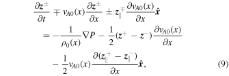
where the subscript ∥ stands for the component parallel to  . The parallel components are not coupled linearly to the perpendicular components: if we consider a purely outgoing Alfvén wave initially, with, say,
  , then the parallel components
  remain zero, i.e., they have no source terms. Here we shall note that the parallel component in this case would be associated with pseudo-Alfvén waves, the incompressible vestige of slow waves, which share the dispersion relation with pure Alfvén waves but have perpendicular polarization to these and components parallel to the magnetic field (e.g., Goossens 2003). We will not focus on pseudo-Alfvén waves here and consider just Alfvén waves. Instead, let us investigate the total pressure term, by decomposing it into the gas and magnetic pressure contributions:

The linear contribution of vA2 is  . As we can see, the magnetic pressure term is nonzero linearly only when the parallel components of the Elsässer variables are not vanishing. This will have crucial implications later on. However, for this case, it is just a confirmation of the known fact that pure Alfvén waves present no linear magnetic pressure perturbations. As pure Alfvén waves have no gas pressure perturbations linearly as well, the total pressure term is zero, meaning that the dynamics are described by setting the argument of the divergence in Equation (6) to zero. The linear version of this equation is analogous to the equations derived by Heinemann & Olbert (1980):

where the subscript ⊥ stands for the perpendicular component. These equations describe outward- and inward-propagating pure Alfvén waves that are linearly coupled owing to reflections and completely described by  : they are advected in opposite directions (Hollweg & Isenberg 2007). As we will see shortly, the reason why pure Alfvén waves still exist in this case is the lack of perpendicular inhomogeneities, in the perturbation direction.
2.2. A Plasma with Inhomogeneities Perpendicular to the Magnetic Field
Let us now consider the case of perpendicular structuring. Although density or magnetic field variations in the perpendicular direction are different, in the case of only perpendicular structuring the last term on the rhs of Equation (5) has linear components only along the field, and as we will see, this component does not “feed” the perpendicular component. For similar Alfvén speed gradients, the evolution should not be substantially different. Therefore, we consider magnetic field variations, as then the last term on the rhs of Equation (5) vanishes. We will consider a straight magnetic field that is varying in the  -direction:
  . The linearized Elsässer equations now take the form

where the z subscript stands for the  component of z±. First, we consider a perturbation in the
  component of, say, z+. With only
  perturbed (uniformly along the y-direction), this component is decoupled from the other components, and it travels as a pure Alfvén wave, with different speed on different field lines:

This is the phenomenon of phase mixing (Heyvaerts & Priest 1983): Alfvén waves traveling on neighboring field lines will get out of phase if there is an Alfvén speed gradient across the field lines, leading to a bending of the wave fronts, or in the formulation of, e.g., Ghosh et al. (1998), a refraction of the Alfvén waves to oblique angles. There is no coupling between z±, and the Elsässer variables completely describe the phase-mixed Alfvén waves traveling up (say, z−) or down (z+) the magnetic field lines. As we will see in the following, the  components are coupled linearly to
  in this equilibrium if an initial perturbation in
  has a
has a  -dependence.
Now we will focus on the main subject of this paper, that of inhomogeneities in the wave perturbation direction, perpendicular to the magnetic field, and we will indicate how it leads to a different turbulence phenomenology, that of self-cascading waves. The study of MHD waves in plasmas in which there is an inhomogeneity in the direction of the perturbation has a long history (e.g., Barston 1964; Sedláček 1971; Grossmann & Tataronis 1973), and it is known to lead to the phenomena of MHD surface waves in the case of a discontinuous variation (e.g., Parker 1964, 1974; Roberts 1981; Goossens et al. 1992, 2009), or to quasi/global MHD waves and resonant absorption in the case of a continuous variation (e.g., Chen & Hasegawa 1974; Hasegawa & Chen 1974; Sakurai et al. 1991). A common and much-studied example of surface waves are the surface Alfvén waves in flux tubes (Goossens et al. 2012), which are analogous to surface Alfvén waves on a planar interface in Cartesian geometry, as employed here (Roberts 1981).
We consider initial perturbations to, say, z+ in the  -direction, while z− = 0. We can immediately see a crucial difference between this case and the previously employed cases: now the parallel components of z± are linearly coupled to the
  components through the inhomogeneity by the third term on the left-hand side (lhs) of Equation (12):

where  . Note that the perpendicular components act as sources for the parallel components, but not the other way around:

where  . This can be interpreted as a single wave perturbing both the parallel and perpendicular components. Therefore, the resulting waves necessarily have both z± nonzero, as well as both parallel and perpendicular components. The other crucial difference is that the linear total pressure term is nonzero. We can immediately see this from Equation (7) and our previous discussion on the magnetic pressure term. The resulting waves cause linear total pressure perturbations as they propagate. This is important, as harmonic modes of homogeneous and incompressible plasmas show no total pressure perturbations. Indeed, these waves can only exist owing to the inhomogeneity and can be referred to as surface Alfvén waves in case of a discontinuous variation or quasi/global Alfvén waves or Alfvénic waves in the case of continuous variation (e.g., Goossens et al. 2002). It is the linear total pressure term that couples the perpendicular components of z±. Note that if the initial perturbation in
  has a
has a  -dependence, the linear total pressure term also couples the
  and
and  components, as the
  -dependence of
  implies the
  -dependence of the linear pressure term through Equation (7). Therefore, in the following we analyze the perpendicular component
  instead of the
  and
and  components for a more general presentation, while understanding that
  is nonzero.
It is well known that the surface Alfvén or quasi/global Alfvén waves are propagating wave solutions—that is, unidirectionally propagating while suffering no backward reflections. This hints that the Elsässer variables are coupled and co-propagating, as they both describe a wave propagating in one direction. As we mentioned in the Introduction, this just means that these waves are not pure Alfvén waves any longer, hence they must necessarily be described by both Elsässer variables while propagating (Magyar et al. 2019). In fact, this can be shown, if a Fourier analysis of the perpendicular components is possible in time and in the  -direction:

where for positive k and ω the waves are propagating toward positive x-values in time. For the sake of a more general derivation, let us consider for now a generally inhomogeneous plasma in the perpendicular direction, i.e., ρ0(y, z), B0(y, z). The perpendicular component of the induction equation (Equation (2)) reads

which Fourier-analyzed according to Equations (16) gives

where  is the phase speed determined by the dispersion relation of the specific initial condition. Using
  and
and 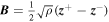 from the definition of Elsässer variables, the Fourier-analyzed induction equation gives

This is an important relation of the perpendicular components of the Elsässer variables. Note that when vph = vA0 = const., as in a homogeneous incompressible plasma, the fields are not coupled. Equation (19) is a very general result. Specifically, it applies to both compressible and incompressible plasmas, as Equation (17) is generally valid. Thus, it connects the perpendicular components of the Elsässer variables in the linear regime in any plasma configuration homogeneous along the magnetic field.
Returning to a magnetic field inhomogeneity along  as considered initially, let us further investigate Equations (15). They show that starting from only
  , the source of
  is the linear total pressure perturbation. A naive interpretation of these equations would lead us to conclude that
  are counterpropagating, since the speeds in front of the advective term are multiplied by ∓1, in direct contradiction with the well-known fact that solutions to Equation (12) are propagating waves that do not display wave reflection. Therefore, the total pressure term has to act in such a way as to cancel the backward advection of
  . However, this cannot be its only function, as both
  should exist. It also acts as a source for
  . Indeed, if we replace the total pressure term in Equations (15) for
  from the equation for
  , we get

If we substitute either  by using Equation (19), we get the important result

which confirms our previous claim that the Elsässer variables both propagate in the same direction, with speed vph. Note that Equation (21) is still valid for a general inhomogeneity across the magnetic field,  . For arbitrary vA0(y, z), vph has no analytical solution. Numerically it can be found by using, e.g., the T-matrix theory (Keppens et al. 1994; Luna et al. 2009, 2010). However, in the case of a discontinuous variation of B0(z), i.e., an interface at z = 0, the solutions to Equation (12) are known (Roberts 1981), and the dispersion relation gives

where the i and e subscripts represent the values above and below z = 0, respectively. Then Equation (21) just describes surface Alfvén waves.
After the realization that a plasma with inhomogeneities perpendicular to the magnetic field admits as linear solutions unidirectionally propagating waves that are necessarily described by both  nonzero and co-propagating, let us get back to the equation describing the nonlinear evolution, now with
  :
:
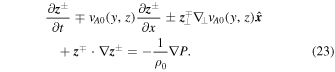
The nonlinear advective term (last term on lhs), responsible for turbulence generation in a homogeneous and incompressible plasma, is still the essential nonlinearity here, still requiring both z± nonzero. However, now wave solutions are described by z± that are co-propagating! This leads to a coherent interaction between z±, which can be interpreted as a self-cascade or self-deformation of unidirectionally propagating waves, a phenomenon that leads to what we call uniturbulence. The coherent interaction differentiates uniturbulence from the counterpropagating wave phenomenology, in which interactions are incoherent deformations of Alfvén waves. There are also other differences between the two turbulence generation mechanisms. The nonlinear deformation of colliding Alfvén waves is an inherently 3D phenomenon, as the waves must collectively vary along both perpendicular directions (Howes & Nielson 2013). This criterion is expressed as  , where
  are the perpendicular wavevectors. In uniturbulence, this is still a valid criterion for the existence of a self-cascade along both perpendicular directions, where one or both of the wavevectors can be given by the plasma inhomogeneity. However, the self-deformation of waves is no longer necessarily 3D. This fact can be seen easily from the properties of surface/global waves arising in inhomogeneous plasmas. These waves generally have a varying perturbation amplitude in the perturbation direction. For example, a linearly polarized (2D) surface Alfvén wave has perpendicular velocity perturbations that decay exponentially away from the interface, resulting in perpendicular gradients of the Elsässer variables. As surface Alfvén waves have both
  , the nonlinear advective term is nonzero. In fact, 1D acoustic waves are well known to self-deform, a process mostly referred to as nonlinear wave steepening or shock formation. The resulting turbulent dynamics is often referred to as burgulence (Frisch & Bec 2001).
3. Numerical Simulations of Uniturbulence
The first numerical demonstration of the phenomenon of self-cascading, unidirectionally propagating waves was presented by Magyar et al. (2017). They considered a setup with multiple random Gaussian density enhancements across the straight magnetic field, while along the magnetic field the plasma was homogeneous. This setup was too complicated to be easily analyzed and understood in simple terms regarding the generation of energy cascade. Here we shall present a simple workable example in which uniturbulence develops.
3.1. Numerical Code, Initial and Boundary Conditions
We run full 3D ideal MHD simulations using the FLASH code (Fryxell et al. 2000; Lee et al. 2009), opting for the third-order unsplit staggered mesh Godunov method (Lee & Deane 2009; Lee 2013) with HLLD solver and mc slope limiter. The code implements constrained transport to keep the divergence of the magnetic field down to round-off errors. An adaptively refined mesh is used, with three levels of refinement for the highest-resolution runs. The base resolution is 64 × 80 × 120 for a domain of size (in user units) 0.6 × 0.1 × 0.15. We found that higher-resolution runs show generation of increasingly smaller scales and more complicated flow behavior, as expected. However, this does not alter our qualitative conclusions. The origin lies in the geometric center of the bottom  slice. As we expect smooth dynamics along the magnetic field, we set a much lower resolution in the
  -direction. We chose to present the results in user units, as the MHD equations are scale invariant. In these units, the magnetic permeability μ is unity. Next, we will present the simple initial conditions of our model. We employ a straight, homogeneous magnetic field
  , with B0 = 1.115. This specific value has no special significance besides normalization purposes. The gas pressure is constant, as required for equilibrium, with the ratio of gas to magnetic pressure β ≈ 7.7. As we solve the full compressible MHD equations, we opted for a high plasma beta in order to minimize the compressible contribution, i.e., as close as possible to the incompressible limit. Our discussion in Section 2 is valid for an incompressible plasma; however, by setting our velocity perturbations much lower than both the Alfvén and sound speeds, we assure that compressible effects are kept at a minimum, i.e., the resulting waves are highly Alfvénic and presenting minimal compressive contributions. Nevertheless, tests with different plasma beta values (from β ≈ 0.02 to 15) indicate that the dynamics perpendicular to the magnetic field are not very sensitive to its value. The density is varying discontinuously at z = 0 from 0.5 to 2.5, while it is constant along the other directions. Although there is a discontinuity at t = 0 in density, this discontinuity is transitioning into a steep gradient once the simulation starts, as we have a nonzero numerical diffusion, inherent to the scheme. The thickness of this inhomogeneous layer is therefore determined by the resolution. We opted for a strong inhomogeneity, as then the nonlinear terms are significantly large (in comparison to linear terms) even for relatively small Mach numbers of the perturbations. Moreover, we opted for an inhomogeneous density and not an inhomogeneous magnetic field as in Section 2 because jumps in magnetic field values are much less stable numerically. As discussed in Section 2, this should not significantly affect the linear perpendicular evolution of the wave; however, it adds an extra nonlinear term. We do not consider any equilibrium flows.
The boundary conditions are the Neumann-type zero-gradient or open conditions in the  -direction for all variables and periodic boundaries in the
  -direction. In the
  -direction, at the bottom we impose a sinusoidal velocity driver polarized in the
  -direction that is varying sinusoidally along the
  -direction:

We set the frequency ω = 2π and the wavenumber ky = 2π/0.1, which corresponds to one wavelength fitting in the  -direction. Without
  variation in the driver, the problem would be 2D, as the
  components are then decoupled, and we would not expect a cascade in both perpendicular directions, as stated in Section 2. We run simulations with two amplitudes: a “low”-amplitude (A ≈ 0.001) and a “high”-amplitude (A ≈ 0.01) driver. The minimum Alfvén speed in the simulation is VA0 ≈ 0.7, while the minimum sound speed is cs0 ≈ 1.26. This shows that the Alfvén and sound Mach numbers are low, 0.014 and 0.008, respectively. At the top boundary in the
  -direction we impose open boundary conditions, in order to allow waves to leave the domain freely. Tests with homogeneous density runs show maximum 1.0% reflection of the incident Alfvén wave energy.
3.2. Simulation Results
We run the simulation for six periods of the driver, that is, until t = 6.0. In Figures 1 and 2, the evolution of the density is shown in a cross section for the high- and low-amplitude drivers, respectively. The second snapshot from the left shows the first maximum displacement, at t = 0.75. While the low-amplitude solution at this time is almost a sinusoidal in the y-direction, in agreement with the linear solution (Roberts 1981), the high-amplitude solution already shows deviations from the linear regime. There are “ripples” appearing on the density surface, as well as overall deformations, indicating that the nonlinear generation of smaller scales is already at work. At later times, we observe increasingly stronger and more complex deformations of the interface for the high-amplitude run, as well as deformations for the low-amplitude run. Note that in the high-amplitude run fluctuations not only affect the interface but also are visibly present in the homogeneous regions around the interface at later times. In Figures 3 and 4, the Elsässer fields are shown in the cross section at different times, for the high- and low-amplitude drivers, respectively. For waves of Alfvénic character propagating along the magnetic field pointing in the x-direction, the dominant Elsässer field is z− (see Equation (19)), while z+ is relatively small. Note that while z− is present in the whole cross section (e.g., at t = 0.75), z+ is mostly confined around the discontinuity. To understand this behavior, let us investigate the wave modes that were excited by the driver. An easier way to do this is by looking at the longitudinal cross section in Figure 5. We distinguish three different characteristic speeds, most easily visible from the first wave front (at t = 0.3). There are two wave fronts traveling with different speeds above and below the interface and a strong “bump” at the interface, which decays away from it, traveling with its own phase speed. The phase speed of this “bump,” as well as its decaying nature, leads us to identify it as a surface Alfvén wave (Roberts 1981). The term “surface Alfvén wave” shall be understood here in the broader sense, as we are not exactly in the incompressible limit, much like in the way it can be used to describe kink waves of solar flux tubes (Goossens et al. 2009, 2012). Therefore, the wave driver excites essentially pure Alfvén waves above and below the interface and a surface Alfvén wave at the interface. As we have seen in Section 2, surface waves present both Elsässer variables while propagating, explaining why z+ is confined mostly around the interface. The reason why not only a surface Alfvén wave is excited is that the driver is not matching the eigenfunction of a surface Alfvén wave. The driver is a spatially independent, uniform forcing, while the surface Alfvén wave has an exponentially decaying behavior away from the interface. The bending of the wave front seen in Figure 5 is essentially the linear process of phase mixing (Heyvaerts & Priest 1983), but for the situation in which the inhomogeneity is in the perturbation direction, discussed in, e.g., Malara et al. (1992) and Ghosh et al. (1998), and is due to the linear advection term in Equation (23). The linear nature of the process is confirmed by the similar evolution for the two different amplitudes in Figure 5. However, the differences seen at later times are revealing: note the fine, small-scale structures evolving in the high-amplitude run across the magnetic field, on top of the bent wave fronts. This small-scale generation is nonlinear in nature, and it is confined to the vicinity of the interface. Also note that while there is a cascade to small scales in the perpendicular direction, the solution remains smooth along the magnetic field, a well-known property of MHD turbulence with a strong guide field (Biskamp 2003). In Figure 6, the linear advection term is plotted against the nonlinear terms. These essential nonlinear terms are the well-known nonlinear advective term (last term on lhs of Equation (23)) and a nonlinear term that is nonzero only in the presence of density gradients (second term on rhs of Equation (5), with vA a perturbation). For the low-amplitude simulation, the nonlinear terms are by far the strongest at the interface, while away from the interface they are negligible. Note the main difference between the two nonlinear terms: the second nonlinear term can only act at the interface, i.e., at the strong density gradient, while the nonlinear advective term is exponentially decaying away from the interface; therefore, it is also acting away from it. This leads to the important observation that surface/global Alfvén waves not only are inducing nonlinear deformations at the interface but also act throughout the plasma and can self-cascade away from the interface. In the low-amplitude case, the nonlinear term involving the density gradient is clearly dominant over the nonlinear advective term and is responsible for the deformation of the interface depicted in Figure 2. Note that the nonlinear term is on average on the order of or less than the linear advection term for the low-amplitude case. In the high-amplitude case, the nonlinearity is initially mostly affecting the interface, but the advective nonlinearity eventually becomes stronger and appears to affect the whole region around the deformed interface. In this case the nonlinear term is on the order of or higher than the linear advection term. Note that in Figure 6 the color bar for the linear advective term is scaled 10-fold between the two runs, while the color bar for nonlinear terms is scaled 100-fold, in accordance with our expectation of the strength of nonlinearity. The growth of the nonlinear advective term observed in Figure 6 is expected as z+ appears to strengthen later in time, as shown in Figures 3 and 4. It is unclear at this point why the enhancement of z+ is taking place. However, it appears to be nonlinear in nature, by comparing the low- and high-amplitude figures. One explanation might be the modification of the eigenfunction of the surface Alfvén wave, due to the deformation of the interface.
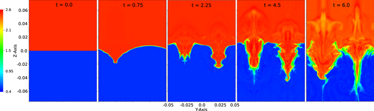
Figure 1. Snapshots of the density in the cross section of the simulation box, at x = 0.5, shown at five different times, indicated on the top of each snapshot, for the high-amplitude run. The first snapshot shows the initial condition, a jump in density at z = 0.
Download figure:
Standard image High-resolution image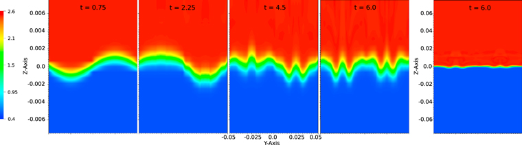
Figure 2. Snapshots of the density in the cross section of the simulation box, at x = 0.5, shown at four different times, indicated on the top of each snapshot, for the low-amplitude run. Note that for the sequence of snapshots on the left, the z-axis was magnified 10-fold. The snapshot at t = 0.6 on the right is not magnified, for comparison. The images were smoothed in order to avoid pixelation due to the limited numerical resolution. This might have introduced some artificial features.
Download figure:
Standard image High-resolution image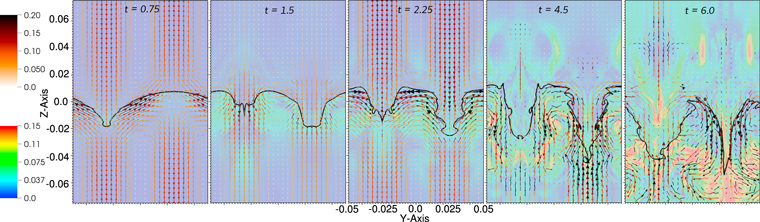
Figure 3. Snapshots of z⊥− (vector arrow field) and  (color plot) in the cross section of the simulation box, at x = 0.5, for the high-amplitude run, shown at five different times, indicated on the top of each snapshot. The black contour shows the deformation of the interface in density. Vector magnitude, besides by length, is also represented by the “orangehot” color table (on top). Vector origin is the middle of the arrows. Values are in user units.
Download figure:
Standard image High-resolution image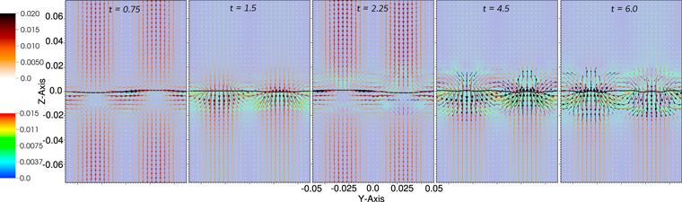
Figure 4. Same as in Figure 3, but for the low-amplitude run.
Download figure:
Standard image High-resolution image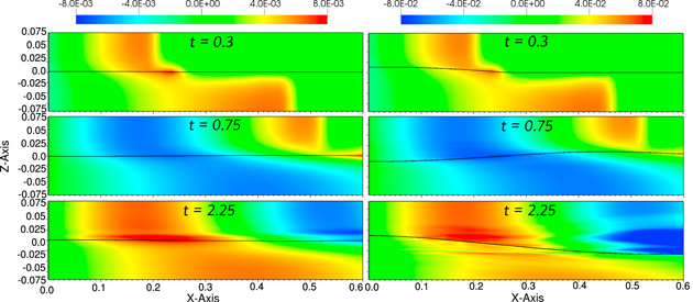
Figure 5. Snapshots of vz in the x–z plane, at y = 0.025, for the low-amplitude (left column) and high-amplitude (right column) runs, shown at three different times, indicated on the top of each snapshot. The black contour shows the position of the interface in density. Values are in user units.
Download figure:
Standard image High-resolution image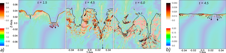
Figure 6. Snapshots of the nonlinear advection plus nonlinear density gradient terms ( , vector arrow field), and linear advection term (
 , color plot), in the cross section of the simulation box, at x = 0.5, shown at three different times, indicated on the top of each snapshot for the high-amplitude run (left) and at t = 4.5 for the low-amplitude run (right). Vector magnitude, besides by length, is also represented by the “orangehot” color table (on top). Vector origin is the tail of the arrows, to better emphasize the location of nonlinearities. Values are in user units.
Download figure:
Standard image High-resolution imageAs we mentioned previously, there is a weak numerical reflection of the propagating waves at the upper, open boundary. Therefore, it is crucial to discuss whether the reflected waves are responsible or can modify the turbulent cascade in the simulation. There are several arguments that dismiss the importance of the reflected waves. First of all, the reflection is very weak (maximum 1% reflected wave energy), and therefore the resulting nonlinear advective term must be very small. Indeed, the nonlinear advective term is on the order of ≈10−6 for the low-amplitude run, at the z-axis boundaries (i.e., farthest from the interface). For comparison, the nonlinear terms in the vicinity of the interface for the low-amplitude run are on the order of ≈10−2. Second, it is also clear in Figures 2–6 that the nonlinearity is mostly affecting the vicinity of the interface, where most of the co-propagating z+ is situated. If the reflected waves would cause a cascade, this should be distributed in the whole simulation, as the whole boundary is driven equally. Last but not least, the reflected waves have the same polarization as the incident waves; therefore, in theory the nonlinear advective term for reflected waves should vanish. Thus, the weak nonlinearity at the z-axis boundaries is also originating from the surface wave, which decays exponentially away from the interface. Still, one could argue that the reflected waves could interact with the surface Alfvén wave, which has a differently polarized eigenvector. However, the co-propagating z+ of the surface Alfvén wave is on average an order of magnitude larger than the reflected z+.
We have also studied the perpendicular spectra of relevant quantities, such as energy, density, Elsässer variables, etc. It is clear that higher wavenumbers are being populated in time; however, we opted not to show these spectra, as the value of the power-law slope might be unreliable. First of all, the available numerical resolution is limiting the extent of the inertial range to about a decade in k-space, restricting the accuracy of the fitting. Second, turbulence might not be fully developed yet at the end of the simulation; therefore, averaging in time for a smoother spectra is not reliable. Lastly, we have noticed that the perpendicular spectra of the perturbations along the magnetic field are shallower than those of the perpendicular perturbations. As the amplitude of the induced perturbations along the field depend on the plasma beta, it appears that the slope of the energy spectra also depends on plasma beta. This aspect is very interesting, and further research is needed to clarify this dependence.
4. Discussion and Conclusions
The underlying mechanism of turbulence generation in MHD is generally accepted to be the nonlinear mutual deformation of colliding, counterpropagating Alfvén waves, propagating along some mean magnetic field. This observation is based on the fact that, in the Elsässer formulation of the MHD equations, the nonlinear advective term requires both Elsässer variables to be nonzero. In an incompressible and homogeneous plasma, the two Elsässer variables represent upward- and downward-propagating pure Alfvén waves of arbitrary amplitude, respectively. Hence, the requirement for both Elsässer variables to be nonzero simply means the existence of counterpropagating Alfvén waves in an incompressible and homogeneous plasma. In this paper we show that once inhomogeneities across the magnetic field are accounted for, new modes appear that have properties different from the waves resulting from a normal mode analysis of a homogeneous plasma. The simplest example of these new modes, described in this work, are the incompressible surface Alfvén waves on a planar discontinuity in Alfvén speed across the magnetic field. Of course, the discussion can be generalized to arbitrarily inhomogeneous cross sections, in which case the waves are referred to as global waves. These waves propagate perturbations both along and across the magnetic field and have linear total pressure perturbations, in contrast to the pure Alfvén and pseudo-Alfvén waves. Most importantly here, these waves are necessarily described by both Elsässer variables, while propagating unidirectionally. This should not come as a surprise, as in general once waves are not pure Alfvén waves any more, they represent perturbations in both Elsässer fields. This is valid also for the magnetoacoustic waves in homogeneous, compressible MHD. Therefore, in plasmas that are compressible or inhomogeneous, or both, the requirement for the two Elsässer variables to be nonzero in order to have nonlinear advection has a different physical meaning: this condition is now satisfied also for unidirectionally propagating waves, without the need for counterpropagating waves. In this sense, waves can self-cascade or self-deform nonlinearly, leading to what we term uniturbulence. The self-cascade of waves can be understood as a coherent nonlinear interaction of Elsässer variables (for a discussion, see Velli et al. 1989). This is an important distinction from the well-known counterpropagating wave scenario, where the interactions are incoherent and act for a shorter period, as the waves interacting are advected in opposite directions. From a theoretical point of view, another important difference from the homogeneous case is the presence of an additional term in the evolution equation of Elsässer variables, nonzero only when density inhomogeneities are present. This nonlinear term acts together with the nonlinear advective term, causing additional self-deformation. To illustrate the difference between the two nonlinear terms, one can think of a plasma in which inhomogeneities are given by interfaces of sharp change in density, or contact discontinuities. Then, while the nonlinear advection term has a space-filling character, the nonlinear density gradient term mostly deforms the interfaces, in case of global waves present in the plasma.
In order to test our prediction that unidirectionally propagating waves can self-cascade nonlinearly, we ran full 3D MHD numerical simulations of a simple setup with surface Alfvén waves excited, as a proof of concept. By analyzing the results, it is clear that the surface Alfvén wave initiates an energy cascade, generating smaller scales, and an overall deformation of the initially planar interface. The self-deformation is initially manifested mostly in the interface via the nonlinear density gradient term; however, later on small scales appear in the vicinity of the interface as well, via the nonlinear advection term. It is unclear whether a steady-state turbulence in the statistical sense is achieved or achievable in such conditions as here. We have also noticed a number of interesting properties of the simulated self-cascade, such as the apparent growth of the relatively smaller Elsässer variable over time, or the shallower perpendicular spectra of the velocity and magnetic field perturbation along the magnetic field, which could result in total energy spectra likely depending on the plasma β. However, as the primary goal of the simulations is a proof of concept, we leave these questions open and as subjects for future research. We did not discuss the possibility of equilibrium flows, especially shearing flows along the magnetic field. Even in an otherwise homogeneous plasma, the velocity shear effectively leads to a transverse Alfvén speed gradient, and Equations (12) apply. Therefore, the discussion following Equations (12) is valid also for an Alfvén speed gradient given by a velocity shear. In fact, Hollweg et al. (2013) studied velocity-shear-induced mode coupling of MHD waves and hinted that the resulting wave behavior might lead to coherent interactions and to turbulence.
The evolution of uniturbulence, presented in Section 3, has similarities in appearance to other well-known instabilities relevant for turbulence generation. These are the Rayleigh–Taylor (RT) and Richtmyer–Meshkov (RM) instabilities (I) (Zhou 2017a, 2017b) and the Kelvin–Helmholtz (KH) instability (Chandrasekhar 1961). First, let us focus on the RT and RM instabilities. These instabilities appear at an interface between two fluids of different densities. The trigger is any misalignment between the (total) pressure gradient and density gradient at the interface. This leads to a nonzero baroclinic term, generating vorticity (Shelyag et al. 2011). This vorticity can further enhance the misalignment, leading to the instabilities. The pressure gradient exists either because of hydrostatic pressure in the presence of acceleration/gravity (in RTI) or due to a shock wave traversing the interface (in RMI). The misalignment can result from a perturbation to a planar interface with nonzero wavenumber along it, or a nonplanar interface. In our simulations without gravity, the driven surface Alfvén wave is the only source of acceleration to the interface. Therefore, both the displacement of the interface and the total pressure gradient are the result of the perturbation, meaning that baroclinic terms appear only nonlinearly. This implies that linear surface Alfvén waves are not RT-unstable, in agreement with their dispersion relation (Roberts 1981). Finite-amplitude surface Alfvén waves might still be nonlinearly RT-unstable. Nevertheless, the identification of uniturbulence with nonlinear RTI is not straightforward, as our description in Section 2 is for a constant density plasma, which by definition is not RT-unstable. Still, the nonlinear density gradient term (second term on rhs of Equation (5)) might be associated with the nonlinear RTI. The possibility of a nonlinear instability strengthens our description that uniturbulence is the result of self-deforming or self-cascading waves.
Second, the KHI appears as a result of a velocity shear with an inflection point in a fluid. The surface Alfvén wave solution with nonzero perpendicular wavenumber along the interface presents velocity shears at the interface. In our simulation there are no background flows; therefore, KHI would also have to appear nonlinearly. However, along with a velocity shear, the surface Alfvén wave presents magnetic field perturbations as well, which is known to inhibit the growth of KHI. As such, propagating Alfvén waves are known to be stable to KHI (Heyvaerts & Priest 1983). This does not rigorously translate to KH-stable surface Alfvén waves, but it hints at stability. The velocity shear in the simulations is less than the rms of the induced perpendicular Alfvén speed along the interface, a condition for KH stability (Chandrasekhar 1961). Of course, this condition is not for time-dependent fields, but a complete KH stability analysis is beyond the scope of this paper. Therefore, with the above arguments we cannot rigorously exclude nonlinear KHI. For related studies of KHI in time-dependent flows see, e.g., Barbulescu et al. (2019) and Hillier et al. (2019).
Finally, allowing for a little speculation in this matter, we could say that RTI and KHI arising nonlinearly, as it might occur here, could equally well be described as manifestations of uniturbulence—that is, nonlinear, coherent interactions of Elsässer variables, leading to turbulent flows. This might explain why their morphology seems similar. In summary, the connection between uniturbulence and instabilities is not fully understood, but it is an exciting topic that warrants future research. The analysis presented in Section 2 is for an incompressible plasma. We chose an incompressible MHD description, as uniturbulence is already present. Hence, it can be understood without the complications and extra terms in the equations related to compressibility. However, the solar corona and solar wind are known to be slightly compressible (Bruno & Carbone 2013), and in some cases the nearly incompressible (Zank & Matthaeus 1992, 1993) or fully compressible description may need to be considered. The description of uniturbulence in a compressible plasma is left for future work. Uniturbulence might likely be relevant in plasmas structured across the magnetic field, such as the solar corona and solar wind. Specifically, it could provide an additional cascade rate and therefore enhanced dissipation, especially in open magnetic field regions. Nevertheless, having in mind the coherent nature of the interaction, it might be relevant even in closed magnetic environments, such as coronal loops. Again, future research is needed to determine the importance of uniturbulence as compared to the classical counterpropagating cascade in different plasma environments.
T.V.D. was supported by the GOA-2015-014 (KU Leuven) and the European Research Council (ERC) under the European Union’s Horizon 2020 research and innovation program (grant agreement No. 724326).