Abstract
We study time-dependent relativistic jets under the influence of the radiation field of the accretion disk. The accretion disk consists of an inner compact corona and an outer sub-Keplerian disk. The thermodynamics of the fluid is governed by a relativistic equation of state (EOS) for multispecies fluid that enables us to study the effect of composition on jet dynamics. Jets originate from the vicinity of the central black hole, where the effect of gravity is significant and traverses large distances where only special relativistic treatment is sufficient. So we have modified the flat metric to include the effect of gravity. In this modified relativistic framework we have developed a new total variation diminishing routine along with a multispecies EOS for the purpose. We show that the acceleration of jets crucially depends on flow composition. All the results presented are transonic in nature; starting from very low injection velocities, the jets can achieve high Lorentz factors. For sub-Eddington luminosities, lepton-dominated jets can be accelerated to Lorentz factors >50. The change in radiation field due to variation in the accretion disk dynamics will be propagated to the jet in a finite amount of time. Hence, any change in radiation field due to a change in disk configuration will affect the lower part of the jet before it affects the outer part. This can drive shock transition in the jet flow. Depending on the disk oscillation frequency, amplitude, and jet parameters, these shocks can collide with each other and may trigger shock cascades.
Original content from this work may be used under the terms of the Creative Commons Attribution 4.0 licence. Any further distribution of this work must maintain attribution to the author(s) and the title of the work, journal citation and DOI.
1. Introduction
Astrophysical jets are collimated outflows of plasma associated with various Galactic and extragalactic sources, such as neutron stars, young stellar objects (YSOs), gamma-ray bursts (GRBs), microquasars, and active galactic nuclei (AGNs). These jets span over a wide range of energy and length scales. For example, the jets of YSOs travel a distance of several parsecs, while AGN jets are observed to remain collimated for a range of hundreds of kiloparsecs. In terms of jet kinetic luminosity, YSO jets have luminosity of the order 1032 erg s−1, while the GRB jets can reach up to 1052 erg s−1. Since the advent of radio telescopes in the era of modern astronomy, the understanding of these ubiquitous objects has improved significantly, but there is no consensus about the formation, composition, and collimation of these objects (Harris & Krawczynski 2006). Black holes (BHs), which sit in the heart of microquasars and AGNs, do not have hard surfaces, and therefore the origin of the jet should be the accreting matter itself. Interestingly, simultaneous radio and X-ray observations show a strong correlation between different spectral states of accretion disks and jets states in microquasars (Gallo et al. 2003; Fender et al. 2010; Rushton et al. 2010), which indicates that the jet originates from the accretion disk. Moreover, the jet is launched from the inner part (less than 100 Schwarzschild radius or r g ) of the accretion disk (Junor et al. 1999; Doeleman et al. 2012). The illusive corona, i.e., the source of hard power-law radiation, has been identified as the inner hot part of the accretion disk in many different models (Shapiro et al. 1976; Chakrabarti & Titarchuk 1995; Gierlinski et al. 1997). Therefore, the compact corona may be responsible for the jet activity. Additionally, the jet that originates from a region very close to the BH horizon will travel through the radiation field of the disk and should certainly be influenced by it.
In recent years, numerical simulations of relativistic jets have played a crucial role in explaining the nonlinear dynamics of the system. There are many studies that investigate the propagation of supersonic jets (Walg et al. 2014; Martí 2019; Seo et al. 2021a). These simulations present a global picture of the jet with a forward bow shock, backflow of the fluid, and multiple shocks within the jet beam. Moreover, the role of magnetic field in the jet formation and collimation has also been studied (Sheikhnezami et al. 2012; Fuentes et al. 2021; Komissarov & Porth 2021). But the numerical simulations of radiatively driven outflows and jets are very limited, in spite of the fact that the interaction between the radiation field and plasma is not a new subject. The equations of radiation hydrodynamics have been developed by many authors (Mihalas & Mihalas 1984; Kato et al. 1998; Park 2006; Takahashi 2007), and these equations have been used extensively in steady-state investigations of the radiatively driven outflows around compact objects. Icke (1989) used a relativistic equation with near disk approximation of the radiation field above a Shakura–Sunyaev disk (Shakura & Sunyaev 1973) to obtain an upper limit of jet terminal speed. Fukue (1999) showed that under the influence of radiation arising from disk corona, the jet can achieve significant collimation. Hence, the radiation not only accelerates the jet but also helps in collimation. Later, Fukue et al. (2001) showed that electron–proton jets can reach relativistic terminal speeds by considering a hybrid disk with inner advection-dominated accretion flow (ADAF; Narayan et al. 1997) and an outer Keplerian disk. The disk model considered by Chakrabarti & Titarchuk (1995), with a mixture of matter with sub-Keplerian and Keplerian angular momentum, showed that a sub-Keplerian disk (SKD) can go through a shock transition and create a hot and compact post-shock disk, which can act as an illusive corona. It may be noted, however, that an inner, puffed hot disk acting like a corona has been suggested by other authors as well (Shapiro et al. 1976; Gierlinski et al. 1997). Numerical simulations of advective disks show that the extra thermal gradient term in the hot post-shock region automatically generates the bipolar outflows (Das et al. 2014; Lee et al. 2016), which can be accelerated by the radiation field of the disk. In the relativistic radiation hydrodynamic regime, investigations by Chattopadhyay (2005) and Vyas & Chattopadhyay (2017, 2018, 2019) clearly highlight that the radiation field of the accretion disk plays a significant role in the acceleration of the jets. In addition to these steady-state investigations, there are limited numerical simulations in the nonrelativistic regime (Chattopadhyay & Chakrabarti 2002a; Chattopadhyay et al. 2012; Raychaudhuri et al. 2021; Joshi et al. 2022). To study the effect of radiation on winds, there are some simulations of line-driven winds (Proga et al. 2000; Yang et al. 2018), but the line-driven force is only effective when the wind is cold, so the line-driven force is not applicable in hot plasma, which is being considered in this paper.
In this paper, we have made an attempt to understand the dynamics of the jet in the time-dependent radiation field of the accretion disk. The steady-state investigations by Vyas & Chattopadhyay (2017, 2018, 2019) and Ferrari et al. (1985) have shown that the radiation field can produce internal shocks in jets, but how these shocks evolve under a time-dependent radiation field is not yet known. Thus, the central theme of this paper is to investigate the formation and evolution of these shocks in relativistic jets due to its interaction with the radiation field of the accretion disk. We study jets that are launched with subsonic speeds close to the central BH. Since the jets are launched close to the BH, one has to consider the effect of gravity at the jet base. However, due to the huge length scales jets traverse, in most parts gravity is negligible and special relativity suffices. Previous studies like Ferrari et al. (1985) and Vyas et al. (2015) used the Newtonian or pseudo-Newtonian potential as an additive source term for gravity in the special relativistic Euler equation, but this destroys the conservative nature of equations of motion, which is essential in the Eulerian upwind numerical schemes we are using. Hence, we include the gravity by modifying the special relativistic metric itself and thereby retaining the conservative form of the equations of motion. The presence of gravity makes the jet transonic, while we avoid general relativistic details. The temperature of the jet varies by a large value, so we use a relativistic equation of state (EOS) in our analysis given by Chattopadhyay & Ryu (2009). This EOS (abbreviated as CR) handles the variation of the adiabatic index and also allows us to study the effect of plasma composition on the jet solution.
The internal shocks in the jet are identified as bright knots in the jets. These shocks are the sites for particle acceleration in the jets, resulting in nonthermal emissions. The jet models with shock are very popular and have been used to explain the outbursts in microquasars (Kaiser et al. 2000), AGNs (Walg et al. 2014), and GRB jets (Rees & Meszaros 1994). A shock very close to the jet base around a stellar-mass BH was considered to explain the high-energy power-law emission (Laurent et al. 2011). Numerical simulations of jets show that the shocks form in the jet beam whenever a fast-moving supersonic plasma catches up with a slower-moving flow ahead. It is well known that the radiation field accelerates by pushing the jet material. However, due to relativistic effects, radiation would also decelerate the jet close to the disk via a process called radiation drag (Icke 1989; Fukue 1999; Chattopadhyay & Chakrabarti 2002b; Chattopadhyay et al. 2004; Chattopadhyay 2005). Therefore, if the disk radiation is time dependent, can it accelerate the jet at lower altitudes to trigger shocks by crashing the lower-altitude, faster blobs onto the slower portion of the jet above it? As these jet shocks are time dependent, how does the shock strength evolve in time? If the disk is oscillating, can the resulting time-dependent radiation field produce multiple shocks? Further, would these shocks collide with each other and generate shock cascades? How would the jet solutions depend on the baryon fraction of the jet? In this paper, we address these questions.
In Section 2, we present the assumptions and governing equations used in this paper. In Section 3, we outline the methodology to obtain the solutions. Section 4 is devoted to explaining and discussing the key findings of this paper. In Section 5, we conclude our work.
2. Assumptions and Governing Equations
We study the jets driven by the radiation field of an accretion disk around a nonrotating BH. We do not include the accretion disk directly in our study; the disk plays a supportive role by supplying the radiation field. All the disk parameters used in our study are required only for the calculation of the radiative moments. We have not explored the direct connection between disk and jet generation; instead, we assume that the jet injected with a finite subsonic initial velocity and some initial temperature. In this study we restrict our calculations for a relativistic nonrotating (uϕ
= 0), axisymmetric (∂/∂ϕ = 0), on-axis (θ = 0) jet. We assume a conical geometry of the jet with a narrow opening angle. The energy-momentum tensors for jet material ( ) and radiation field (
 ) are given as

where uα represents the components of four-velocity, lα are the direction cosines, and Iν is the specific intensity of the radiation field. In addition, dΩ is the solid angle subtended by the field point on the jet axis to the source point on the accretion disk, ρ is the rest mass density of fluid, and h is the specific enthalpy of the fluid, which is related to the internal energy density e and pressure p as

The spacetime metric is given by

where gtt is given as

We have used the geometric unit system where 2G = M B = c = 1, M B is the mass of the BH, G is the gravitational constant, and c is the speed of light. The information of gravity is supplied through gtt , somewhat in the spirit of weak-field approximation, although the Φ is given by the Paczyńsky–Wiita potential (Paczyńsky & Wiita 1980), instead of the Newtonian one. This way, we retain the conservative nature of equations of motion. In this unit system, the Schwarzschild radius (r g = 2GM B /c2) is the unit of length and t g = 2GM B /c3 is the unit of time.
The equations of motion for relativistic radiation hydrodynamics have been derived before (Park 2006; Takahashi2007); here we present only a brief description to obtain the equations of motion. The continuity equation that represents the conservation of mass flux is given as  . The equations of motion are essentially the conservation of energy-momentum tensor, or
  .
.
A conical jet along the axis of symmetry implies that ur is the only significant component of the four-velocity, and conservations of mass flux and energy-momentum tensor can be written as a set of three conservation laws:


Here v is the three-velocity of the jet. The four-velocity (ur ) can be written in terms of v as ur = γ v, where γ is the Lorentz factor given as γ2 = − ut ut = 1/(1 − v2). The conserved quantities D, M, and E are the mass density, momentum density, and total energy density in the laboratory frame, respectively, given as (see also Ryu et al. 2006; Seo et al. 2021b)


Gr and Gt are the components of the radiation force, which under the present set of assumptions are explicitly given as (Mihalas & Mihalas 1984; Kato et al. 1998; Park 2006)

where
Here ρe
is the total lepton density,  , and Erd, Frd, and Prd are the zeroth moment or energy density, first moment or the flux, and second moment or the pressure of the radiation field, respectively.
To solve the equations of motion (5)–(7), we need an additional closure relation that relates the thermodynamic variables h, p, and ρ. This closure relation is known as the EOS. In this study, we consider an EOS for relativistic multispecies fluid proposed by Chattopadhyay & Ryu (2009) (abbreviated as CR EOS). CR EOS is a very close fit to the exact one given by Chandrasekhar (1939). The CR has already been used for different astrophysical problems (Cielo et al. 2014; Singh & Chattopadhyay 2019; Sarkar et al. 2020; Joshi et al. 2021, 2022).
The EOS is given as

where
In Equations (13) and (14) ρ is the mass density of fluid given as  , where
  , η = m
e
/m
p
, and
, η = m
e
/m
p
, and  , n
p
, m
e
, and m
p
are the electron number density, proton number density, electron rest mass, and proton rest mass, respectively. Θ = p/ρ is a measure of temperature, and τ = 2 − ξ + ξ/η. The expression for sound speed is given as
, n
p
, m
e
, and m
p
are the electron number density, proton number density, electron rest mass, and proton rest mass, respectively. Θ = p/ρ is a measure of temperature, and τ = 2 − ξ + ξ/η. The expression for sound speed is given as

Here N is the polytropic index given as
The polytropic index is a function of temperature. Hence, we do not need to supply it as a free parameter. From Equation (16) one can see that for higher values of temperature Θ ≫ 1, N → 3, and N → 3/2 for Θ ≪ 1. The adiabatic index is related to the polytropic index as

2.1. Steady-state Equations of Motion
In the steady state, we impose ∂/∂t ≡ 0 on equations of motion (5)–(7). Integrating Equation (5) then leads to the mass-outflow rate,

where  is the cross section of the jet. The energy balance equation or first law of thermodynamics is given by
  , which gives the temperature gradient
Integrating the above and combining with Equation (18) gives the adiabatic relation (see also Kumar et al. 2013; Joshi et al. 2022)

where
Since interaction of radiation with the jet in the Thomson scattering regime is isentropic, the entropy-outflow rate is a constant along a streamline in the steady state but discontinuously jumps up in case there is a shock transition in the jet. The relativistic Euler equation ![$[({\delta }_{\mu }^{r}+{u}^{r}{u}_{\mu }){\left({T}_{M}^{\mu \nu }+{T}_{R}^{\mu \nu }\right)}_{\nu }=0]$](https://content.cld.iop.org/journals/0004-637X/933/1/75/revision1/apjac70deieqn11.gif) can be simplified to the following form:
can be simplified to the following form:

where the last term in the numerator  is the radiation momentum deposition term, which can be simplified to the form

We can integrate Equations (22) and (19) to obtain another constant of motion for steady flow known as the generalized relativistic Bernoulli parameter ( ),
),

We consider an advective-type accretion disk (Fukue 1987; Chakrabarti 1989; Lee et al. 2011; Kumar & Chattopadhyay2017) for this study. Figure 1(a) shows a typical cartoon diagram for the disk and jet system. As mentioned earlier, the disk plays only a supportive role in our calculations by supplying the radiation field. Depending on the accretion rate, advective disks have moderate to low radiative efficiency (Sarkar et al. 2020). The disk has two components, an inner puffed-up post-shock disk (PSD) and an SKD. The sub-Keplerian part of the disk supplies the soft photons, and the geometrically thick PSD, also known as corona, supplies the hard photons. This type of disk structure can mimic hard to hard-intermediate spectral states in microquasars. The PSD terminates at the horizon, but we take the inner edge of the corona at 1.5 r g , as the disk is expected to emit negligible radiation from a region within it. Numerical simulations of advective accretion flows suggest that the SKD is flatter than the PSD (Lee et al. 2016) and the ratio of height to the horizontal extent of corona can vary from 1.5 to 10, so we take a semivertical angle θsk = 85° for the SKD, and the intercept of the SKD on jet axis is taken to be d0 = 0.4h s , where h s is the height of the corona taken as h s = 2.5x s . The outer edge of the SKD is taken at xo = 3500. The details of obtaining the radiative moments are presented in Chattopadhyay & Chakrabarti (2000), Chattopadhyay (2005), and Vyas et al. (2015); here we present only a brief description.
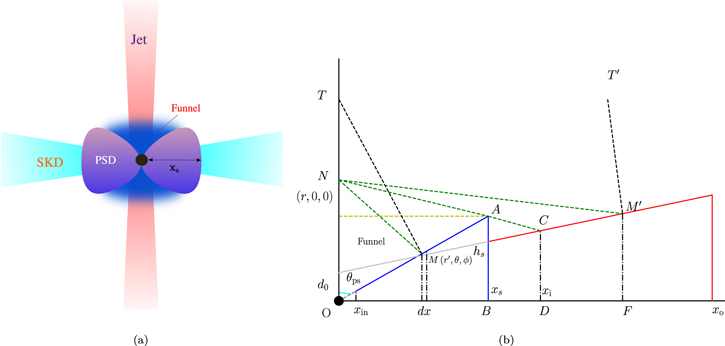
Figure 1. (a) Schematic representation of the disk–jet system. The shock location (x
s
) and various components of the disk–jet system are shown. The blue region marks the funnel above the PSD. (b) Cartoon diagram to show the cross-sectional view of the disk. The blue portion is the inner compact corona. The SKD is shown with solid red lines. N is the field point on the jet axis where radiative moments are calculated. M and  are the source points on the corona and the SKD.
Download figure:
Standard image High-resolution imageIn Figure 1(b) we have shown a cross-sectional view of the disk–jet system. M and  are the source points on the PSD and SKD, respectively. TM and
  are the local normals on the disk surface. We calculate the radiative moments on the field point N. The inner edge of SKD is at x
s
, but due to the shadow effect (Chattopadhyay 2005), the observer at N sees the SKD starting from xi
given as
are the local normals on the disk surface. We calculate the radiative moments on the field point N. The inner edge of SKD is at x
s
, but due to the shadow effect (Chattopadhyay 2005), the observer at N sees the SKD starting from xi
given as

We need the intensities of various disk elements to obtain the radiative moments of respective disk components. In the SKD, we assume the synchrotron emission (Shapiro & Teukolsky 1983) to be the dominant emission mechanism,
where Bsk, Θsk, nsk, and x represent magnetic field, local dimensionless temperature, electron number density, and horizontal distance from the central object, respectively. We assume a stochastic magnetic field in the SKD with a constant magnetic-to-gas-pressure ratio pmag = β pgas. The general definitions of radiative moments are
and at each field point (e.g., N) these quantities have to be computed from both the sources SKD and PSD. All the components of the radiation moments should ideally be numerically computed in Equation (C1). The details of computing these numerically are given in Vyas et al. (2015) and also in Appendix C of this paper.
However, numerically computing the radiative moments in the simulation code at every cell and at every time step would slow down the code significantly. So we fitted the numerically computed radiative moments (Equations (C2)–(C8)) with approximate analytical functions (Equations (D1)–(D3) for the SKD and Equations (D6)–(D8) for the PSD in Appendix D), which depend on disk parameters like x
s
, h
s
, and xin. The sub-Keplerian accretion rate controls the position of x
s
(Equation (A1)) and luminosities (Equations (B3)–(B4)) of the disk components. The comparison between the moments obtained from numerical integration (solid, dashed, and dashed–dotted lines) and the analytical fitted functions (red, green, and cyan open circles) for xs = 15 is shown in Figure 2. The fitting is good, and the advantage is that any time variation of  will produce a time-dependent radiation field. But the moments are given as analytical functions and need not be numerically computed at every cell and at every time step. It may be noted that
  obtained from Equations (D1)–(D3) and (D6)–(D8) for a given
  are used in Equation (12).
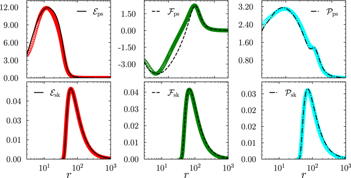
Figure 2. The radiative moments from the PSD and SKD (excluding the constant factors). Lines (solid, dashed, dashed–dotted) represent the correct numerically integrated moments, and open circles (red, green, and cyan) represent moments obtained by fitting functions.
Download figure:
Standard image High-resolution image3. Method of Obtaining Solutions
3.1. Steady-state Solutions
The steady-state solutions are obtained by simultaneously integrating Equations (22) and (19). The jet at its base is hot and slow and therefore subsonic. The jet is powered by the thermal gradient term and the radiative term against gravity and becomes supersonic at some value of r. In other words, jets are transonic in nature, and at some point rc called the sonic point, the flow velocity vc crosses the local sound speed ac . At rc , dv/dr → 0/0 gives the sonic point conditions


From Equation (29) we obtain the temperature (Θc ) at the sonic point, and dv/dr is obtained by using L’Hôpital’s rule. We integrate Equations (22) and (19) inward and outward starting from sonic points to obtain the solutions. The steady-state solutions provide the injection values for the simulation code.
3.2. Time-dependent Solutions and Numerical Setup
We perform the time-dependent calculation using a relativistic total variation diminishing (TVD) routine. The TVD scheme introduced by Harten (1983) is a second-order, Eulerian, finite-difference scheme, which was initially proposed to solve the set of hyperbolic, nonrelativistic hydrodynamic equations. However, many relativistic numerical codes have been built based on the same philosophy (see Martí & Müller 2003, 2015, for details). A relativistic TVD code to incorporate the CR EOS has been built before (Ryu et al. 2006; Chattopadhya et al. 2013). The detailed description of the code is presented in Ryu et al. (2006); here we present only brief details.
The set of Equations (5)–(7) can be written in the form

with the state and flux vectors given as

and the source term S as
The set of Equation (30) is solved in two steps. In the first step, the state vectors
q
at the cell center i at a given time step n are updated using the modified fluxes  calculated at cell boundaries,

where
where
Here
Explicit forms of eigenvalues λk,i , eigenvectors L and R , and flux limiters gk,i , γk,i+1/2, and Qk are given in Ryu et al. (2006). In the second step, the radiation and curvature terms are added as source terms in the updated values of state vectors. The next step consists of recovering the updated primitive variables (ρ, v, p) from the updated conserved variables D, M, and E, which is done by inverting Equations (8)–(10). These equations, along with the EOS, can be expressed as a polynomial of γ, given as
where  . We solve Equation (36) using the Newton–Raphson method to obtain γ, and once γ is known, the primitive variables can be obtained as


Since v, γ, E, and M are known, using Equations (9) and (10), the pressure p is obtained as the root of a cubic equation
We employ a continuous inflow boundary condition at the injection cell and outflow boundary conditions at the outer boundary using ghost cells. In this time-dependent study, we want first to obtain the steady-state solutions as is predicted by theoretical analytical investigations. And then we want to study the influence of accretion disk oscillation on the jet dynamics, while keeping the injection parameters the same as the steady-state values.
3.2.1. Time-dependent Disk as Observed by an Inertial Observer on the Axis
In this paper, the time dependence of the jet is not imposed through the injection parameters, but by making the radiation field from the accretion disk time dependent. In microquasars, quasi-periodic oscillations (QPOs) are observed in hard X-rays associated with the oscillation of the inner part of the accretion disk (Nandi et al. 2012). If there is a fluctuation of the accretion rate  at the outer edge of the disk, the fluctuation would travel inward. The time variability of the accretion rate
  is given in Equation (A2), which induces a sinusoidal variation in the size of the PSD or x
s
, which is of the form
is given in Equation (A2), which induces a sinusoidal variation in the size of the PSD or x
s
, which is of the form

where the oscillation is about a mean xs0 (distance OG of Figure 3) with an amplitude of A (NG = GN ), as shown in Figure 3, and frequency f
s
. The information about the disk fluctuation propagates at the speed of light to the observer P, i.e., it takes a finite amount of time to reach the jet axis. Hence, the different points on the jet axis see a different disk configuration (see Joshi et al. 2022). In other words, the radiation emitted from
), as shown in Figure 3, and frequency f
s
. The information about the disk fluctuation propagates at the speed of light to the observer P, i.e., it takes a finite amount of time to reach the jet axis. Hence, the different points on the jet axis see a different disk configuration (see Joshi et al. 2022). In other words, the radiation emitted from  at t reaches P after a time t + δ
t (δ
t = l″/c; see Figure 3), and in the same time interval the PSD boundary will move from
at t reaches P after a time t + δ
t (δ
t = l″/c; see Figure 3), and in the same time interval the PSD boundary will move from  to
to  . Therefore,

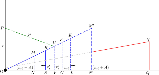
Figure 3. Schematic representation of time-dependent disk configuration as seen by an observer P on jet axis. xs0 is the mean position of the shock and  is the actual position of the shock at time t.
Download figure:
Standard image High-resolution imageThe position x s is updated after each time interval dt, which is determined by the TVD code. Hence, we can write

where s = 0.5(vs,t + vs,t+dt ) is the average velocity in the time interval between t and t + dt. The instantaneous velocities can be obtained from Equation (40),

From Equations (41) and (42) we can write

We solve Equation (44) at each r and at every time step to obtain the x s as seen by the observer there, and the corresponding radiative moments are calculated using the analytical estimates of the radiative moments (Equations(D1)–(D8)).
4. Results
4.1. Code Verification
The relativistic Riemann problem is a great tool to test the time-dependent hydrodynamic code, and the special relativistic TVD code with CR EOS was indeed tested against the analytical relativistic Riemann problem (see Joshi et al. 2021). To check the correctness and accuracy of the code in the relativistic radiation hydrodynamic regime in the presence of gravity, currently we compare the numerical result with the steady-state semianalytical radiatively driven relativistic jet solution. In Figure 4 we have shown the solutions obtained from the TVD code marked by open red circles and analytical solutions shown by solid black lines. The evolution of various variables like flow velocity v, Mach number M (≡v/a), Θ (which is the measure of temperature), and adiabatic index Γ along the jet is shown in panels (a)–(d), respectively. The SKD accretion rate  is taken to be 10, which produces a PSD with x
s
= 8.212, and disk luminosity is l = 1.0. The SKD accretion rate
is taken to be 10, which produces a PSD with x
s
= 8.212, and disk luminosity is l = 1.0. The SKD accretion rate  and disk luminosity l are in units of the Eddington accretion rate (
 ) and the Eddington luminosity (
 ), respectively. The injection parameters with which the jet is launched are chosen from the analytical solution and are given by vin = 0.065, Θin = 0.037, and rin = 5.0. The sonic point of the steady-state solution corresponding to these parameters is at rc
= 14.0. We divide the computational domain of total length 1000r
g
into 6000 uniform cells. It may be noted that the simulation of outflows requires higher resolution compared to accretion disk simulations because of the presence of sharp gradients at outflow injection boundaries. The comparison shows that the code regenerates the solution very accurately. The adiabatic index of the jet at the base is moderately relativistic but becomes nonrelativistic at large r, which suggests that the use of CR EOS to describe the thermodynamics of the jet is appropriate.
), respectively. The injection parameters with which the jet is launched are chosen from the analytical solution and are given by vin = 0.065, Θin = 0.037, and rin = 5.0. The sonic point of the steady-state solution corresponding to these parameters is at rc
= 14.0. We divide the computational domain of total length 1000r
g
into 6000 uniform cells. It may be noted that the simulation of outflows requires higher resolution compared to accretion disk simulations because of the presence of sharp gradients at outflow injection boundaries. The comparison shows that the code regenerates the solution very accurately. The adiabatic index of the jet at the base is moderately relativistic but becomes nonrelativistic at large r, which suggests that the use of CR EOS to describe the thermodynamics of the jet is appropriate.
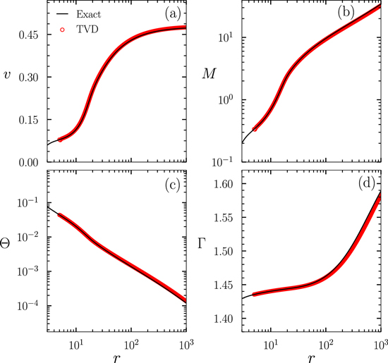
Figure 4. Comparison between the steady-state solutions obtained from the TVD code (red open circles) and the analytical method (solid black lines), for vin = 0.065, Θin = 0.037, and rin = 5.0. The jet is electron–proton or ξ = 1.0 fluid.
Download figure:
Standard image High-resolution image4.2. Effect of Disk Luminosity on Jet Solution
In Figure 5(a), we compared solutions of electron–proton (ξ = 1) jets corresponding to different disk luminosities, all starting with the same injection parameters vin = 0.018, Θin = 0.063, and rin = 2.5. These injection parameters are taken from a thermally driven steady-state solution characterized by the sonic point location rc
= 15.0. Each curve represents a thermally driven jet (solid black curve) and jets driven by disk luminosities l = 0.53 (solid red), l = 1.0 (dashed–dotted blue), and l = 2.4 (dashed green), all in units of Eddington luminosity. The terminal speed of the thermally driven jet is v
T
= 0.13c. It is expected that higher disk luminosity would accelerate the jets to higher vT. And indeed Figure 5(b) shows that vT increases with l, to the extent that an electron–proton jet for sub-Eddington disk luminosity (l < 1) may reach mildly relativistic speeds (vT ∼ 0.4c–0.5c), while for the super-Eddington luminosities the jet can achieve relativistic terminal velocities. Interestingly, higher l suppresses the jet velocity v in the funnel-like region above the PSD. From Figure 2, it is clear that the radiative flux  in the funnel-like region between the inner walls of the PSD. So with higher l, the
  will actually suppress the jet speed within the funnel region, although at higher altitudes it would push the jet. Therefore, vT increases with l.
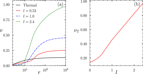
Figure 5. The effect of radiation on the jet solutions. Velocity profiles for various solutions with different disk luminosities are plotted in panel (a), and panel (b) shows the terminal velocities.
Download figure:
Standard image High-resolution image4.3. Effect of Jet Composition
The interaction between the jet plasma and radiation is dominated by Thomson scattering, so the amount of momentum transferred to the jet will be higher for the lepton-dominated jet, which can be clearly seen from Equation (12). To study the effect of composition, we fix injection and disk parameters, and the solutions are obtained for various values of ξ. In Figure 6(a) we have plotted the velocity profiles of various jet solutions, with the injection parameters vin = 0.11, Θin = 0.22, and rin = 2.0. The disk luminosity is l = 0.82. The radiation term Rr for solutions with a higher fraction of protons (higher ξ) will be weaker, resulting in lower terminal speeds. But the radiation term inside the funnel is negative, so the lower magnitude of Rr means a low value of deceleration, so the proton-dominated flows turn out to be faster at lower r. So the electron–proton jet (ξ = 1.0), plotted with the dashed–dotted blue line, is fastest near the jet base. The composition parameter significantly affects the terminal velocities, which can be clearly seen in Figure 6(a). The terminal velocity for electron–positron flow (ξ = 0), plotted with the dashed green line, is vT = 0.999876, and the corresponding terminal Lorentz factor is γT = 63.51. In the right panel we have plotted the variation of terminal Lorentz factor γT with respect to the jet composition for luminosities l = 0.82 (dashed-red), l = 0.66 (dashed–dotted blue), and l = 0.54 (solid blue). These results clearly suggest that the interaction of disk radiation with the jet plasma can play a crucial role in the acceleration of the jet. In contrast to the electron–proton jets, the lepton-dominated jets can reach ultrarelativistic speeds even for the sub-Eddington luminosities.
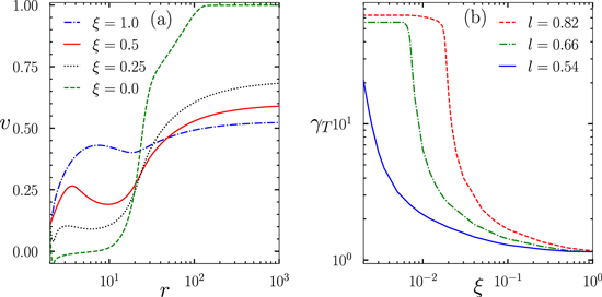
Figure 6. (a) The velocity profiles for different plasma compositions of the jet. Panel (b) shows the variation of terminal Lorentz factor with respect to composition parameter for various disk luminosities.
Download figure:
Standard image High-resolution image4.4. Jet Solutions under the Time-dependent Radiation Field
To study the effect of disk oscillation on jet dynamics, we first obtain a steady-state solution corresponding to injection parameters of the steady-state analytical solution. The steady-state time is taken to be t = 30000 tg
. In Figures 7 and 8 the injection parameters are vin = 0.076, Θin = 0.064, and rin = 3.0. The disk luminosity for the steady-state configuration is l = 0.597, and the outer edge of the PSD is at x
s
= 12.0 (obtained from Equation (A1)). The velocity (v), Mach number (M), and net radiation force term (Rr
) for the steady-state solutions are plotted (blue solid curve) in Figures 7(a1), (b1), and (c1), respectively. The sonic point for steady-state solution is at rc
= 13.0. Once the steady-state solution is obtained, we induce a variability in  (Equation (A2)) such that it imposes an oscillation on x
s
with the amplitude A = 7.0, about the equilibrium value xs0 = 12, and with the time period being T = 2000t
g
. In this study we have taken the frequency and amplitude of oscillation as free parameters. As
(Equation (A2)) such that it imposes an oscillation on x
s
with the amplitude A = 7.0, about the equilibrium value xs0 = 12, and with the time period being T = 2000t
g
. In this study we have taken the frequency and amplitude of oscillation as free parameters. As  decreases, x
s
moves outward and the net disk luminosity decreases, resulting in a weaker radiation field (compare blue and red curves in Figures 7(c1)–(c5)). The magnitude of the net radiative force term ∣Rr
∣ for x
s
> xs0 is smaller than the steady-state values (blue) and is larger for x
s
< xs0. So in the funnel region, v is higher when x
s
> xs0 but eventually produces a jet whose vT is weaker and vice versa. Figures 7(a2), (b2), and (c2), show the solution for the configuration when the accretion disk is brightest and the flow is suppressed to remain subsonic within the funnel. However, the flow velocity is boosted in the range 20 < r < 40. The accelerated jet material encounters the slowly moving outer domain (r > 40). As the supersonic fluid is resisted by relatively slower fluid ahead, it drives a shock in the jet, shown in Figure 7(a3). The formation of shock further reduces the downstream velocity of the fluid, and as a result, we can see the formation of multiple shocks in the flow, namely, S1, S2, and S3 as shown in Figure 7(a4). The shock S1, being faster, catches up and collides with the shock in front of it (S2), shown in Figure 7(a5). In Figure 8 we have plotted the zoomed-in region of jet domain 300 < r < 800 to highlight the changes in mass density (ρ) distribution due to collision of the shocks. Figures 8(e1)–(e5) show two shocks S1 and S2 that collide and are plotted in the epoch between Figures 7(a4) and (a5). Figures 8(e6)–(e10) clearly show that the collision results in a cascade effect and induces additional shocks in the flow. Of course, if the oscillation is stopped, the jet eventually returns back to its steady state.
decreases, x
s
moves outward and the net disk luminosity decreases, resulting in a weaker radiation field (compare blue and red curves in Figures 7(c1)–(c5)). The magnitude of the net radiative force term ∣Rr
∣ for x
s
> xs0 is smaller than the steady-state values (blue) and is larger for x
s
< xs0. So in the funnel region, v is higher when x
s
> xs0 but eventually produces a jet whose vT is weaker and vice versa. Figures 7(a2), (b2), and (c2), show the solution for the configuration when the accretion disk is brightest and the flow is suppressed to remain subsonic within the funnel. However, the flow velocity is boosted in the range 20 < r < 40. The accelerated jet material encounters the slowly moving outer domain (r > 40). As the supersonic fluid is resisted by relatively slower fluid ahead, it drives a shock in the jet, shown in Figure 7(a3). The formation of shock further reduces the downstream velocity of the fluid, and as a result, we can see the formation of multiple shocks in the flow, namely, S1, S2, and S3 as shown in Figure 7(a4). The shock S1, being faster, catches up and collides with the shock in front of it (S2), shown in Figure 7(a5). In Figure 8 we have plotted the zoomed-in region of jet domain 300 < r < 800 to highlight the changes in mass density (ρ) distribution due to collision of the shocks. Figures 8(e1)–(e5) show two shocks S1 and S2 that collide and are plotted in the epoch between Figures 7(a4) and (a5). Figures 8(e6)–(e10) clearly show that the collision results in a cascade effect and induces additional shocks in the flow. Of course, if the oscillation is stopped, the jet eventually returns back to its steady state.
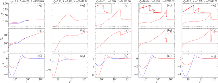
Figure 7. The evolution of jet solution under the influence of disk oscillations. The variation of velocity (panels (a1)–(a5)), Mach number (panels (b1)–(b5)), and radiative term (panels (c1)–(c5)) is plotted at different epochs. The steady-state solution (blue solid) is obtained for steady luminosity l = 0.597 and steady PSD configuration at xs0 = 12. The PSD oscillation is for amplitude A = 7 and time period T = 2000t g about an equilibrium value xs0 of the size of PSD.
Download figure:
Standard image High-resolution image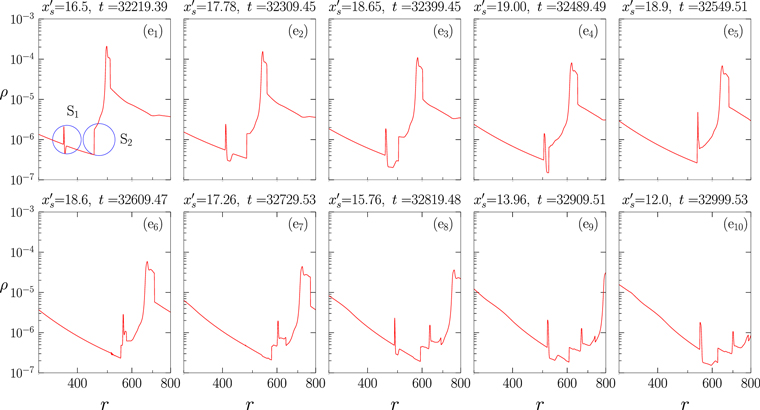
Figure 8. Density distribution ρ of the jet at various time steps are plotted to the collision between shock S1 and S2 in panels (e1)–(e5). Panels (e6)–(e10) show the ρ after the collision. The PSD oscillation is the same as in Figure 7.
Download figure:
Standard image High-resolution imageIn Figures 9(a) and (b) we plot the variation of positions of jet shocks S1 and S2 and their compression ratios R as a function of time t. Figure 9(a) shows that the slope of the rsh versus t graph is steeper for the shock S1, which clearly suggests that the speed of S1 is faster than that of S2 and ultimately catches up with S2 at rsh ∼ 535. The compression ratio is the ratio of post-shock and pre-shock densities (R = ρ+/ρ−), which is an indicator for the strength of the shock. Panel (b) shows that both the shocks are very strong, but the variation of R with respect to time has a complicated profile for both shocks. The shock S1 becomes stronger as it moves outward, reaching a maximum value of R ∼ 4.4, and gradually starts to slow down. The compression ratio for the second shock S2 reduces initially but starts to increase to reach a maximum value of R ∼ 4.55, and then it becomes weaker.
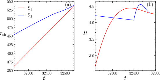
Figure 9. The variation of shock positions and the compression ratio R are plotted in panels (a) and (b), respectively, for jets as described in Figures 7 and 8.
Download figure:
Standard image High-resolution imageA closer look at Equation (23) indicates that the radiative effects are strong for the colder flows and relatively weaker for the hotter jets. Hence, we also study a hotter jet solution with injection parameters vin = 0.14, Θin = 0.226, and rin = 2.0, considered from the analytical jet solution for a steady disk configuration x
s
= 11.02 and l = 0.664. The velocity (v) and Mach number (M) variation for the steady-state solution is plotted in Figures 10(a1) and (b1) with the solid blue line. The amplitude of oscillation for x
s
is A = 6.0, and the time period of oscillation is T = 500t
g
. In Figures 10(a1)–(b5) we have plotted the jet solution for different values of x
s
as  is varied with time. So the variation of
  determines the l and x
s
at various t. One of the distinct features of this hotter solution is that it harbors an internal shock very close to the jet base (rsh ∼ 10) as shown in Figures 10(a3) and (b3), and this shock is transported outward as the jet solution evolves in time. Since this is a hot jet near the base, radiative force is less effective, and it would be thermally accelerated to supersonic speeds within the first few Schwarzschild radii and more importantly within the funnel. A supersonic jet has low temperature, and radiative terms become significant. Inside the funnel Rr
< 0, so resistance to the supersonic part of the jet drives a shock. This type of shock was not present in the previously shown solution because the jet base was relatively colder, and so the jet was strongly decelerated to remain subsonic throughout the funnel region just above the PSD. It may be noted that such shocks in jets have been invoked to explain high-energy emissions (Jamil et al. 2008; Laurent et al. 2011).
determines the l and x
s
at various t. One of the distinct features of this hotter solution is that it harbors an internal shock very close to the jet base (rsh ∼ 10) as shown in Figures 10(a3) and (b3), and this shock is transported outward as the jet solution evolves in time. Since this is a hot jet near the base, radiative force is less effective, and it would be thermally accelerated to supersonic speeds within the first few Schwarzschild radii and more importantly within the funnel. A supersonic jet has low temperature, and radiative terms become significant. Inside the funnel Rr
< 0, so resistance to the supersonic part of the jet drives a shock. This type of shock was not present in the previously shown solution because the jet base was relatively colder, and so the jet was strongly decelerated to remain subsonic throughout the funnel region just above the PSD. It may be noted that such shocks in jets have been invoked to explain high-energy emissions (Jamil et al. 2008; Laurent et al. 2011).
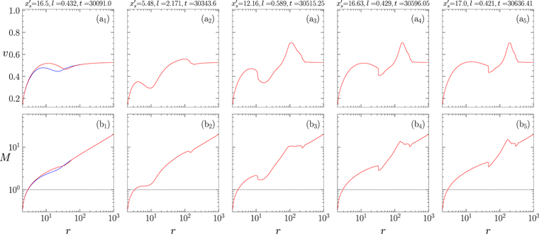
Figure 10. The time-dependent jet solution corresponding to injection parameters vin = 0.14, Θin = 0.226, and rin = 2.0.
Download figure:
Standard image High-resolution image4.5. Effect of Disk Oscillation Frequency on Jet Solutions
We have discussed earlier in Section 3.2.1 that the information regarding the time variability of the disk (or portions of it) does not reach the entire jet simultaneously. The photons take some finite amount of time to reach different parts of the jet. Hence, the different points on the jet axis at a time t would see the outer edge of the PSD at different locations. If the oscillation frequency of the disk is very low, then the emitted photons can reach to a larger distance of the jet axis before the outer edge of the PSD reaches a new position. In Figure 11 we have compared the jet solutions corresponding to two different frequencies of the disk oscillation. The injection parameters are vin = 0.076, Θin = 0.064, and rin = 3.0 (same as Figure 7). The time period of the disk oscillation is T = 2000 tg for the solution plotted with a solid red line and T = 105 tg for the solution plotted with a dashed green line. Here the jets are compared at the same disk configuration (same l and x s ). The time at which the disk reaches the same l and x s will be different for the two frequencies and has been shown in each panel. Assuming an M B = 10 M⊙, these time periods correspond to oscillation frequencies 5 Hz and 100 mHz, respectively. The microquasars show the QPOs at various frequencies. For example GRO J1655–40 (with central mass ∼7 M⊙) itself shows the QPOs at various frequencies extending from 0.1 to 10 Hz (Remillard et al. 1998; Chakrabarti et al. 2008). Hence, as a representative case for two different frequencies of disk oscillations we have taken the values 100 mHz and 5 Hz. These results clearly indicate that for low-frequency oscillations in the disk the transient features (shocks) are not present in jet solutions. The jet velocity gets boosted up or slowed down depending on the disk configuration, but the solutions remain smooth throughout the domain.
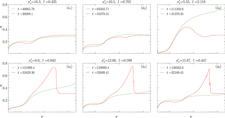
Figure 11. The evolution of jet solutions (v vs. r) under the influence of disk oscillations of frequencies fs = 2000t g (solid red) and 105 t g (dashed green). The injection and disk parameters are similar to Figure 7. The two jet solutions in each panel correspond to the same x s and l, and the time in which the disk configuration is similar for the two cases is mentioned in the panels.
Download figure:
Standard image High-resolution image5. Discussion and Conclusion
In this paper, we studied the relativistic jets driven by the radiation field of advective-type disks. The jet gains momentum supplied by the radiation field. We use relativistic radiation hydrodynamic equations along with a relativistic EOS to study the jet properties. We use the steady-state analytical solutions to verify our time-dependent code. The steady-state solutions also provide us the injection parameters at the jet base to be used in time-dependent cases. The accretion disk plays an auxiliary role in our study by supplying only radiation. It may be noted that we have considered sub- and supercritical accretion rates to compute the radiation field above the disk. In the advective disk regime, supercritical accretion rates may make the inner part of the accretion disk optically slim (1 < optical depth ≲ few), although higher infall velocity keeps the outer part of the disk optically thin. In such cases, the radiative transfer equation needs to be solved to compute the radiative intensity emitted by the disk, especially from the inner part. Since the disk plays an auxiliary role and is not part of the computational domain, we considered simplifying assumptions to compute the radiation field. We show the effect of radiative acceleration on the terminal speeds of the jets. The supercritical disks accelerate the electron–proton jets to terminal Lorentz factor γT ≳ 4. The jets driven by subcritical disks also achieve reasonable relativistic speeds. The EOS allowed us to study the solutions corresponding to various plasma compositions. We found out that the electron–positron jets can be accelerated to ultrarelativistic speeds (γT > 50). The radiative acceleration is quite impressive; however, we have not considered the effect of back-scattered photons onto the jet base, which may inhibit the jets. That might slightly lower such impressive terminal speeds as we have obtained. In a nutshell, it may be summarized that the net radiation force (Rr
) is negative inside the funnel region above the PSD and therefore opposes the jet expansion, but above the funnel region the net radiative force is positive and therefore the jet is accelerated. The time dependence of the jet is imposed by the time dependence of the radiation field. It may be recalled that Kumar et al. (2014) studied the radiatively and thermally driven outflows from advective accretion disks, and they have shown that the radiative momentum deposition has a more significant effect on jet acceleration than conversion of thermal energy to kinetic energy. Moreover, they also found out that for a given rin (jet base), vin is higher for higher luminosity, but difference in sound speed or Θin is imperceptible. Hence, we have fixed the jet base for this study. It may be noted that we have checked that by imposing a 20% fluctuation of vin with a frequency similar to that of the oscillating x
s
, it produces imperceptible change in the jet solution; therefore, keeping the jet base values fixed was reasonable. As x
s
decreases from its steady-state value, l increases, the funnel becomes smaller, so there is larger acceleration at a smaller r, this faster region of the jet eventually is opposed by the slower-moving outer jet, which eventually develops into a shock. Therefore, an oscillating radiation field in the funnel-like region above the PSD produces shocks in the jet. The cold jet solution does not harbor a shock very close to the jet base, but jets with higher initial temperatures can have an internal shock very close to the jet base (rs
∼ 10). We have shown that the shocks can collide with each other and create multiple shocks after collision, giving rise to shock cascade. We also showed that the production of shocks in jets can also depend on the frequency of oscillation of x
s
or  . Oscillations with higher frequency are likely to produce jet shocks compared to oscillations with lower frequency. In this work, we showed how the radiation field of the accretion disk can affect a jet in a complicated manner. The radiation field of the disk can produce mildly relativistic to highly relativistic jets, and we have also shown that disk oscillations give rise to the production and collision of shocks in jets.
We thank the anonymous referee for valuable comments that improved the quality of the paper.
Appendix A: Sub-Keplerian Accretion Rate and the Size of the PSD
The size of the PSD is related to the sub-Keplerian accretion rate (Vyas et al. 2015)
We give a perturbation in  given as

which results in a sinusoidal oscillation in shock position with a frequency fs
.  is the mean value of accretion rate, and A1 and A2 control the amplitude of oscillation in
  . For example,
  , A1 = 3.6872, and A2 = 1.313 results in a sinusoidal oscillation in shock position with mean shock position x
s
= 12, and amplitude of oscillation is A = 7.
, A1 = 3.6872, and A2 = 1.313 results in a sinusoidal oscillation in shock position with mean shock position x
s
= 12, and amplitude of oscillation is A = 7.
Appendix B: Luminosity of Disk
The luminosities of disk components are obtained by numerically integrating the emissivity over the disk volume

where i represents the disk component (i = SKD or PSD) and li
is the luminosity in units of Eddington luminosity. Ii
is the synchrotron emissivity (erg cm−3 s−1), and  is the Comptonization parameter fitting function.
  for the SKD, and for the PSD it is given as (Kumar et al. 2014)
The disk luminosities are approximated by the algebraic functions given as


Appendix C: Numerically Computed Radiative Moments from the SKD
The radiative moments with relativistic transformations on the jet axis due to the SKD are given as in Vyas et al. (2015). It may be noted that

In the following we present the expressions of radiative moments computed from the SKD (e.g., Qsk) and PSD (e.g., Qps). One needs to follow Figure 1(b) to get a proper reference of the following equations:
where
where  is a constant given as
  . Here γsk is the Lorentz factor, ϑi
is the ith contra variant component of three-velocity of accreting matter, and li
are direction cosines. The temperature at the outer edge of the SKD Θ0 is taken to be Θ0 = 0.2.
. Here γsk is the Lorentz factor, ϑi
is the ith contra variant component of three-velocity of accreting matter, and li
are direction cosines. The temperature at the outer edge of the SKD Θ0 is taken to be Θ0 = 0.2.  represents the accretion rate of the SKD in units of Eddington accretion rate
  . ϑsk is the radial velocity of the accretion disk estimated from freefall velocity (see Vyas et al. 2015). The specific angular momentum λ0 at the outer edge is taken to be λ0 = 1.7.
The specific intensity of the PSD (Chattopadhyay & Chakrabarti 2002b) is given by Ips = lps LEdd /π Aps, where Aps and LEdd are the surface area of the PSD and Eddington luminosity, respectively, and the luminosity of the PSD lps is in units of LEdd . The exact forms of radiative moments from the PSD are
where  is a constant given as
  . Equations (C2)–(C8)) are computed numerically.
Appendix D: Analytical Estimation of Radiative Moments
In the simulation code, we use the analytical estimates of radiative moments (mentioned in Equation (C1)); the explicit expressions for these analytical functions are given below.
The functions that mimic the radiative moments from the SKD are given as

where

Function A(r, x) is given as

and factors  (i = 1, 2, 3) are given as

The algebraic functions that mimic radiative moments from the PSD are given as

where 
where 
Functions P1(r, x), P2(r, x), and P3(r, x) are given as

where  and B3(x
s
) =− 0.022x
s
− 0.056/xs + 1.311.
and B3(x
s
) =− 0.022x
s
− 0.056/xs + 1.311.