Abstract
We studied the unique kinematic properties in massive filament G352.63-1.07 at 103 au spatial scale with the dense molecular tracers observed with the Atacama Large Millimeter/submillimeter Array. We find the central massive core M1 (12 M⊙) being separated from the surrounding filament with a velocity difference of  and a transverse separation within 3″. Meanwhile, as shown in multiple dense-gas tracers, M1 has a spatial extension closely aligned with the main filament and is connected to the filament toward both its ends. M1 thus represents a very beginning state for a massive, young star-forming core escaping from the parental filament, within a timescale of ∼4000 yr. Based on its kinetic energy (3.5 × 1044 erg), the core escape is unlikely solely due to the original filament motion or magnetic field but requires more energetic events such as a rapid intense anisotropic collapse. The released energy also seems to noticeably increase the environmental turbulence. This may help the filament to become stabilized again.
Original content from this work may be used under the terms of the Creative Commons Attribution 4.0 licence. Any further distribution of this work must maintain attribution to the author(s) and the title of the work, journal citation and DOI.
1. Introduction
Star-forming clouds can cause several prominent dynamical consequences. One is the escaping and spreading of young stars toward the surrounding space, which has caught increasing attention during recent years (e.g., Tobin et al. 2009; Kraus et al. 2017; Cantat-Gaudin et al. 2019; Herczeg et al. 2019; Swiggum et al. 2021). The stars tend to be gradually drifting over the entire cloud, forming a similar but more extended spatial distribution (Großschedl et al. 2018; Jerabkova et al. 2019; Kuhn et al. 2020; Ward et al. 2020; Gupta & Chen 2022). This provides a unique proxy to inspect the cloud morphology and mass distribution. Furthermore, based on the recent Gaia-based measurement of the trigonometric parallax and stellar proper motion, one can explore the spatial-velocity structure with an unprecedented accuracy and a historical perspective (e.g., Szegedi-Elek et al. 2019; Galli et al. 2020; Roccatagliata et al. 2020; Krolikowski et al. 2021; Dharmawardena et al. 2023; Ha et al. 2022; Kounkel et al. 2022; Tu et al. 2022; Duan et al. 2023). These works have largely improved our understanding of the dynamical condition and evolutionary trend of the star-forming clouds.
As one critical but incomplete aspect of this study, the initial condition of the escaping young stars is still not widely inspected. With the exception of some extremely high-velocity stars (10–102 km s−1) ejected from n-body (n ≥ 3) interactions (Ducourant et al. 2017; Fernandes et al. 2019; Bally et al. 2020; Rivera-Ortiz et al. 2021), the stellar motions could also be affected by their dense-gas structures. Young stars could directly inherit the turbulent field of the gas structure (Ha et al. 2021; Krolikowski et al. 2021; Gupta & Chen 2022; Quintana & Wright 2022) and obtain further acceleration due to the gravitational instability or other interactions among the parental filaments or clumps (Stutz & Gould 2016; Getman et al. 2019; Kim et al. 2019; Zamora-Avilés et al. 2019; Sharma et al. 2020; Álvarez-Gutiérrez et al. 2021). Stutz & Gould (2016) proposed one particular scenario where the filament in Orion A could have an oscillation that drives the young stars toward transverse directions, eventually forming a broadened stellar distribution in parallel with the filament. But in all these studies, the young stars are either totally separated from the filaments or have dissipated the surrounding gas (e.g., Jerabkova et al. 2019; Gupta & Chen 2022). So we still need to investigate the initial dynamical condition when young stellar objects (YSOs) are leaving their parental structures.
G352.63-1.07 is a massive, young star-forming region at a precisely measured distance of D = 690 pc (Chen et al. 2021, hereafter Chen21). It contains several massive cores aligned on a dense filament. As shown in Chen21, the filament has actively ongoing dynamical features, including prominent outflows and mass transfer flows, which induced bright shock emissions. However, due to the limited molecular tracers and sensitivities, the gas motion among the cores and filaments is still undetermined. In this work, we explored the gas motion using optically thin lines, which demonstrate the unique tendency of the escaping massive core M1. The observed data is described in Section 2. The global dense-gas and velocity distribution is reported in Section 3. The dynamical origin and the time-energy properties of the gas motion are discussed in Section 4. A summary is given in Section 5.
2. Observation
G352.63-1.07 (G352 hereafter) is observed with the Atacama Large Millimeter/submillimeter Array (ALMA) in the ATOMS survey (Liu et al. 2020, 2022). The observation was performed with both Compact 7 m Array and the 12 m array (C43-2 or C43-3 configurations) in Band 3. The restored data cube has an average beam size of  . The antenna baselines can cover the extended structures with a scale up to ∼100″. The channel width and noise level vary with different spectral windows. The H13CO+, CCH, and
  (1-0) lines have Δvchan = 0.2 km s−1 and σrms = 5 mJy beam−1 (0.15 K). The HCO+ (1-0) has Δvchan = 0.1 km s−1 and σrms = 9 mJy beam−1 (0.25 K). The CH3OH (211 − 110) lines have vchan = 1.4 km s−1 and σrms = 2 mJy beam−1 (0.08 K). The more detailed observing conditions are presented in Liu et al. (2020).
3. Results
3.1. Filament and Cores
Figure 1(a) shows the 3 mm continuum emission and the integrated H13CO+ (1-0) emission (moment 0). Compared to the chemically fresh molecules CCH and HC3N (Chen21, Figure 3 therein), the H13CO+ emission is more concentrated toward the inner region of the filament structures. It shows an S-shaped compact filament. The six major cores (Chen21) are clearly resolved therein. The line intensity decreases toward M4 and M5, which could be due to the gas dissipation caused by their outflows (Appendix B).
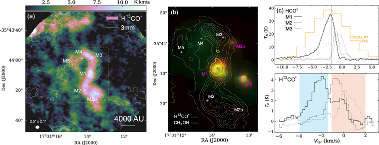
Figure 1. (a) The velocity-integrated intensity of the H13CO+ (1-0) line (false-color) and 3 mm continuum. The contour levels are 4σrms (1.6 mJy beam−1) to 84σrms (peak) in step of 16σrms. (b) The H13CO+ and CH3OH emission regions around the main filament, overlaid on the IRAC-RGB image (3.6, 4.5, and 8.0 μm bands). The H13CO+ contours are 15%–90% in 15% steps of the peak intensity (8.5 K km s−1). The CH3OH contours are 10%–90% in 20% steps of the peak intensity (18.7 K km s−1). The dashed circles label the area of each core. (c) Upper and lower panels: the spectra at the selected core centers. The blue and red shaded areas indicate the velocity ranges of the two velocity components, respectively. The vertical dashed line denotes the division between the blueshift (core M1) and main-filament components.
Download figure:
Standard image High-resolution imageFigure 1(b) shows the H13CO+ emission overlaid on the Spitzer/IRAC three-band color image (GLIMPSE survey; Benjamin et al. 2003; Churchwell et al. 2009). Among the dense cores, only M1 has a compact IR source. M2 to M5 are all absent of IR point sources. The other two IR sources (M3b and M6) are located on the western side of the filament. The IRAC color magnitudes for M1 are [3.6]–[4.5] = 2.1 and [5.8]–[8.0] = 1.0, which are similar to the color of Class-0 YSOs (Megeath et al. 2012). M1 is also detected in 6.7 GHz methanol maser but undetected in 6–8 GHz radio continuum emission above the noise level of 3–8 mJy beam−1 (Walsh et al. 1998). This indicates M1 to have a deeply embedded young massive star. It has not yet caused significant ionization to the surrounding medium. Figure 1(b) also shows the CH3OH (2-1) emission. It has a compact morphology concentrated at M1.
The molecular spectra at the three inner cores are shown in Figure 1(c). The H13CO+ (1-0) exhibits a noticeable double-peak profile at M1. The two components have a separation of vblue − vred = −1.8 km s−1. M2 and M3 both have a single-velocity component within vlsr = ± 0.3 km s−1, which are close to the redshift component at M1. The HCO+ and CH3OH line profiles are less resolved owing to high optical depth and low spectral resolution, respectively. Nevertheless, we can still see these two lines inclined to the blueshift side. We also examined the other two dense-gas tracers CCH and  (1-0) (Figure 3). They have similar velocity components to the H13CO+ (1-0). The molecular lines all indicate prominent blueshift component at M1.
3.2. Physical Parameters and Gravitational Instability
The physical parameters of the cores are presented in Table 1. The details of the calculation are described in Appendix A. All the cores have comparable spatial sizes and are nearly uniformly distributed along the filament, with an average spatial interval of  or (7 ± 1.5) × 103 au.
Table 1. The Physical Properties of the Cores
| Parameters | M1 | M2 | M2b | M3 | M4 | M5 |
|---|---|---|---|---|---|---|
| (Observed) | ||||||
| vlsr (H13CO+) (km s−1) | −2.5 | −0.8 | −0.6 | +0.1 | +1.0 | +1.3 |
| Tex (HCO+) (K) | 37 | 22 | 22 | 22 | 22 | 20 |
| Tb (H13CO+) (K) | 4.0 | 3.0 | 5.0 | 2.1 | 3.7 | 2.6 |
| Δv (km s−1) | 2.5 | 2.3 | 1.8 | 2.2 | 1.8 | 1.7 |
| Radius (arcsec) a | 5 | 4 | 6 | 5 | 4 | 4 |
| (Derived) | ||||||
| Ntot (1023 cm−2) b | 2.6 ± 0.3 | 2.2 ± 0.2 | 2.3 ± 0.3 | 2.4 ± 0.2 | 2.2 ± 0.2 | 2.2 ± 0.2 |
| σtot (km s−1) | 1.1 | 0.9 | 0.8 | 1.0 | 0.7 | 0.7 |
| Mass (M⊙) | 12 ± 2 | 6 ± 2 | 11 ± 2 | 8 ± 2 | 7 ± 2 | 7 ± 2 |
| mcrit (M⊙) | 15 | 13 | 12 | 12 | 11 | 11 |
Notes.
a Average radius deconvolved with the beam size. b Ntot is derived from H13CO+ intensity using Equation (A4). For M4 and M5, the H13CO+ emissions are noticeably dissipated by the outflows. We assumed them to have same Ntot with M3 based on the fact that these cores also have comparable 3 mm continuum emissions.Download table as: ASCIITypeset image
From the observed parameters, we estimated the stability of the cores from the critical mass (Bertoldi & McKee 1992; McKee & Ostriker 2007; Li et al. 2013):

wherein σtot is the effective velocity dispersion (see Appendix A) and MBE and MΦ represent the upper-limit masses to be supported by the turbulence and magnetic pressures, respectively. MΦ depends on magnetic field strength B and mass density ρ0 = μ
mH
n0, which are included in Alfvén velocity of  . For the B value, we referred to the B measurement of the magnetic field in other similar cold and dense filaments (e.g., Ching et al. 2018; Liu et al. 2018). They are found to have a bulk distribution of B = 0.5–1.0 mG. Adopting this range, we can derive MΦ = 0.6 to 1.2 M⊙, which only has a minor contribution to Mcrit. As shown in Table 1, all the cores have
  , which indicates a subcritical state if the turbulence can support them against the self-gravity.
The filament stability can be estimated from the critical line-mass density (Ostriker 1964; Arzoumanian et al. 2013)

From the average line width of Δvfila(H13CO+) = 2.0 km s−1, we can derive σtot = 0.9 km s−1 and (M/l)crit≃390 M⊙ pc. In comparison, the observed total mass (48 M⊙) and length (45″) yield (M/l)obs≃300 M⊙ pc−1. Considering the projection effect, the actual value could be even smaller. Therefore the property of (M/l)obs < (M/l)crit suggests a subcritical state also for the entire filament. The turbulent condition of the filament and cores should have a close interplay with other dynamical features including the core collapse and escaping motion, as discussed in Section 4.
4. Discussion
4.1. Resolving the Velocity Components
As shown above, the filament has an overall smooth and compact morphology. The transfer flows (Chen21) and outflows seem to only have a limited influence to the main filament. As seen in optically thin lines, the blueshift motion of M1 is still the most conspicuous feature over the entire structure. Its dynamical origin should be further inspected.
Figure 2(a) to (c) shows the H13CO+ (1-0) emission in four different velocity channels. The ALMA 3 mm and the Submillimeter Array 1 mm (Chen21) dust continuum emissions are also plotted in Figure 2(d) and (e) for comparison. Figure 2(f) presents the position–velocity (PV) plot of the H13CO+ along the filament. It shows that the blue component is mainly in the velocity range from −4 to −1 km s−1 and has a spatial extension from offset = −16″ to +6″. In order to inspect the gas motion, we plot the emission region in two velocity intervals, denoted as low- and high-velocity components, or LVC and HVC, respectively. We plot their emission regions in Figure 2(a) to (c). One can see that the LVC is peaked at M1 and has a weak elongation toward M2, while the HVC is more confined around M1. Their morphologies are both largely different from the outflow lobes (Appendix B). They should both trace the dense-core motion instead of outflow.
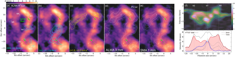
Figure 2. (a)–(e) Contours: emission region of the H13CO+ (1-0) line in three velocity intervals. The background image is the H13CO+ emission in (−1.5,+1.5) km s−1 (red-center component). For the blue-wing component, the contour levels are 4, 6, and 8 times of the rms level (0.3 K km s−1). For the other components, the contour levels are 10%–90% in 20% steps of the peak intensity, which is 15, 11, and 3 K km s−1 for the blue-center, red-center, and red-wing, respectively. The green arrows label the mass transfer flow directions onto the main filament (Chen21). The green circles label the possible arrival points of the transfer flows onto the filament. (f) PV plot and intensity profile along the major axis of the main filament. The sampling direction is labeled in dashed line in panel (a). The vertical dashed lines denote the projected offset of the three dense cores on the sampling direction. The horizontal dotted line represents the average systemic velocity of the filament.
Download figure:
Standard image High-resolution imageThe filament component is mainly in the velocity range of (−1.5,+1.5) km s−1. Its emission region (false-color image in Figure 2(a) to (e)) almost traces the entire gas structure and shows a noticeable gap at M1 center. The redshift wing component (1.5–2.2 km s−1, yellow contours) includes two separated patches, with one extending from M4 and M5 and another around M3. They could trace the denser gas affected by the outflow or transfer flow. Around M1, there are no evident redshift features at v > 1 km s−1. The dust continuum emissions (Figure 2(a), two right panels) show an overall similar spatial extent with the H13CO+ filament but have a compact intensity peak rightly at M1, which is ∼3 times more intense than the remaining filament.
The spatial correlation of the velocity components can also be inspected from their intensity profiles as shown in Figure 2(f) (lower panel). The dust continuum profiles (dashed and dotted lines) rightly follow the blueshift component (blue solid line). They all have a shoulder-like decreasing trend from M1 to M2. This coherency suggests that the dense core M1 should be mainly associated with the blueshift gas.
The gap on the filament is more clearly seen in the intensity profile (red line in Figure 2(f), lower panel). It rightly coincides with the M1 center of both the dust continuum and the blueshift H13CO+ profiles. For the H13CO+ emission, if considering the total intensity profile (black solid line), the blueshift component would nicely fill the gap, making the intensity profile of the entire filament much more flattened.
The CCH emission regions of the two components are shown in Figure 3(a). The PV diagram of CCH is shown in Figure 3(b). The emission regions and PV diagram of the  are shown in Figure 3(c) and (d), respectively. The lower intensity around M1 along the filament can also be seen in CCH (Figure 3(a) and (b)). Although its blue component is more extended than that of H13CO+, it is still mainly concentrated at the central cavity of the filament. The
  emission is more concentrated at M1, so the central intensity decline is not evident. But from its PV diagram, one can still see a comparable velocity separation of v − vlsr = − 2 km s−1 between the blueshift component and the main filament. And it is also closely overlapped with the H13CO+ and CCH spectra for the blueshift peak (Figure 6(c)). The three molecular lines thus consistently suggest the blueshift component to be the dominant one at M1. In other words, the dense core is having a bulk motion relative to the rest of the filament.
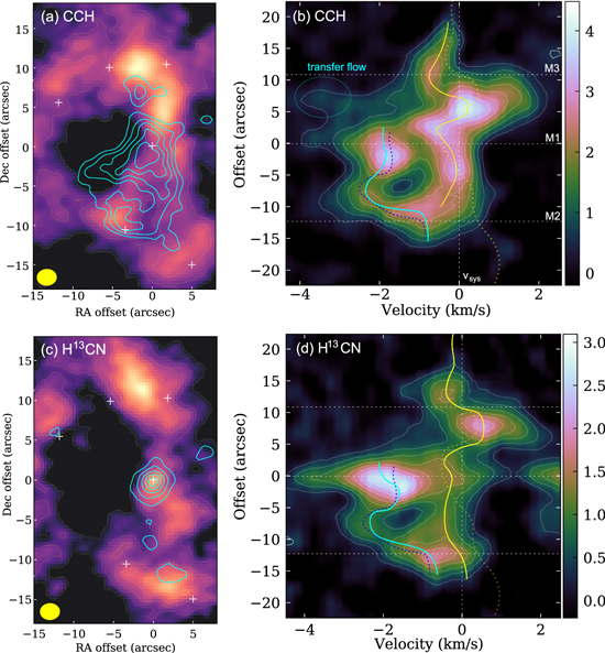
Figure 3. Left column: the emission regions of the blue- (contours) and redshifted (false-color) components in CCH and  (1-0) lines. The contour levels are 20%–90% of the peak intensity. Right column: the PV diagrams of the two molecular lines. the
  emission at vlsr = 2–4 km s−1 is from another hyperfine component (HFC) of F = 1–1. The HFCs of
  are separated for 6–7 km s−1 and would not blend with each other. The CCH (1-0) emission shows an additional small blueshift wing around M3, which should correspond to the transfer flow onto the filament (Chen21). This feature is not seen in other lines probably because of their lower optical depths.
Download figure:
Standard image High-resolution imageBased on their spatial and velocity features, M1 and the main filament could have two possible configurations. M1 can be either leaving the filament on the front side or moving toward it from behind. From the PV plot (Figure 2(b)), one can see the blue component connected to the main filament both toward north and south, around offset = +5″ and −15″, respectively. The PV diagrams of the CCH and  (1-0) lines (Figure 3, right column) show the similar connection feature between M1 and the main filament in the two directions. M1 should thus be originally formed in the filament and have obtained the blueshift motion only during the recent time.
4.2. Driving Force of the Blue Component
The multiple velocity components in G352 are comparable to other filaments with prominent kinematical features. As shown in previous studies, undisturbed linear filaments tend to have moderate fluctuation of ∣v − vsys∣ ≤ 1.0 km s−1 around their internal cores (e.g., Punanova et al. 2018; Bhadari et al. 2020). More complicated fiber-composed filaments also have similar velocity variation within 1 km s−1 (Hacar et al. 2017; Clarke et al. 2018). Stronger kinematical features of several kilometers per second are seen in filaments with collapse (Henshaw et al. 2014; Chen et al. 2019; Ren et al. 2021; Cao et al. 2022; Li et al. 2022) or interactions (Shimajiri et al. 2019; Anathpindika & Francesco 2021). The velocity fluctuations in G352 resembles those most active ones. The blueshift motion (−2 km s−1) and its spatial scale (5″ or 3500 au) lead to a gradient of ∼250 km s−1pc−1, which resembles those most intensely collapsing filaments (e.g., Peretto et al. 2013; Montillaud et al. 2019; Beuther et al. 2021; Hu et al. 2021; Cao et al. 2022).
In collapsing or fiber-composed filaments, the global velocity field is often entangled with the individual core motions. It is therefore uncertain if the cores are co-moving with the filament or already separated. In comparison, G352 presents an example of clearly separated velocity components. In fact, the main filament is also inclined to the blueshift side around M1 toward −0.5 km s−1 (Figure 2(b)). The filament could thus have a co-moving tendency with M1. In particular, as shown in Figure 2(a), the HVC (v = (−4, −3) km s−1) is narrowly confined between the northern and southern segments of the entire filament. This increases the evidence that the core and filament motions are closely related.
The mass transfer flows (Chen21) provide a viable mechanism to initiate the filament collapse. Since the flows are observed from one-sided molecular line wings instead of strong infall signatures, they would provide a moderate mass accumulation to the inner filament (between M2 and M3). Once the mass assembly exceeds the threshold of (M/l)crit or Mcrit , it would possibly induce a major collapse. One can see that the transfer flows exhibit no evident mass assembly at their arrival points on the inner filament (Figure 2). This also indicates that the flows should have a further propagation toward M1.
4.3. Energy Scales of the Gas Components
The filament collapse and core escape can also be examined from their energy scales. From the core mass and its escaping velocity, the kinetic energy of M1 is estimated to be  erg. This would represent a lower limit due to the projection effect. In comparison, the turbulent energy of the entire filament is
  erg. As for the magnetic energy, from the speculated B-range (Section 3.2), we can estimate
  to 8 × 1043 erg. Eturb and EB
values characterize the entire filament. The fraction to reach M1 could be even lower and thus cannot be solely responsible for the core motion.
to 8 × 1043 erg. Eturb and EB
values characterize the entire filament. The fraction to reach M1 could be even lower and thus cannot be solely responsible for the core motion.
The collapsing energy can be estimated as ![${\rm{\Delta }}{E}_{{\rm{p}},\mathrm{coll}}\,={{Gm}}_{\mathrm{in}}^{2}[(1/{r}_{1})-(1/{r}_{0})]$](https://content.cld.iop.org/journals/0004-637X/955/2/104/revision1/apjaced54ieqn17.gif) , which involves the initial and final radii (r0 and r1) of the collapsing mass mcoll. Assuming that the major collapse is taking place between M2 and M3, we can adopt
, which involves the initial and final radii (r0 and r1) of the collapsing mass mcoll. Assuming that the major collapse is taking place between M2 and M3, we can adopt  . Together with the current radius and mass of M1, we derived ΔEp,coll ≃ 6 × 1044 erg, which could be sufficient to accelerate M1.
As seen in the PV diagram (Figure 2(b)), the inner region has a typical line width of Δv ≥ 1.8 km s−1 for both the blueshift component and the main filament. It rapidly declines toward the outer part, reaching a transonic level of Δv ≃ 0.7 km s−1 (σnt = 0.4 km s−1) toward offset = ±20″. The low-Δv areas over the filament could represent the fraction less affected by the collapse. Adopting the average value (0.9 km s−1) in Equation (2), we can derive (M/l)crit≃150 M⊙ pc−1, which is much smaller than (M/l)obs and should reflect the supercritical condition before the major collapse.
Figure 4 shows the velocity distributions over the core and filament in all three lines. The low-turbulence areas with Δv down to 0.6 km s−1 can be seen in all three species. The CCH and H13CO+ emission regions both exhibit the low values down to Δv ≃ 0.7 km s−1, while the higher values mainly appear between M1 and M3. The  line is more concentrated on dense cores, which could be due to its chemical bias toward the protostellar stage. Along the filament, the
  line-width variation is mainly between 1.2 and 1.4 km s−1, which is comparable to average values of CCH and H13CO+ lines.
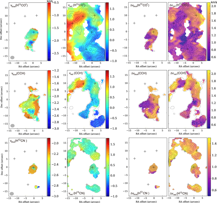
Figure 4. The peak velocity and line-width distributions of the two components as observed in three molecular lines. The velocity ranges to measure the blueshift-core and main-filament components are (−4, − 1.5) and (−1.5, 2) km s−1, respectively. Left two columns: the radial-velocity distributions of the two components. Right two columns: the line-width distributions of the two components.
Download figure:
Standard image High-resolution image4.4. Time Scales of the Gas Motion
Figure 5(a) shows the ridge lines of the main filament and the blueshift component (M1 and southern extension). The two components have a transverse offset of Δsesc = 0″ to 23 along the filament. We plot the Δsesc and ∣vblue − vred∣ profiles along the filament in Figure 5(b). One can see that the two quantities have a coherent variation trend. At M1 and the second velocity peak near M2 (offset = −10″), the velocity and transverse offsets both reach a local maximum.
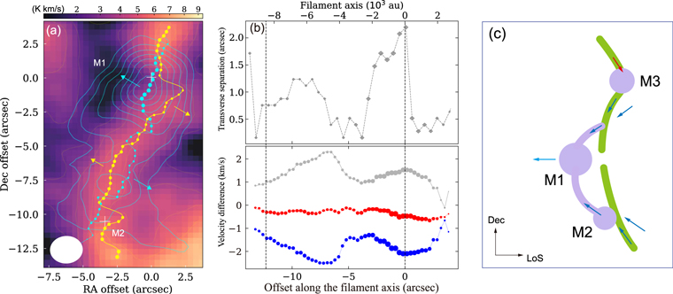
Figure 5. (a) The ridge lines of the two velocity components, blue component in blue line and dots, red-center component (main filament) in yellow line and dots. The dot size is proportional to the integrated intensity. The arrows denote the projected moving direction of each component expected on the sky plane. (b) The transverse offset and velocity difference between the ridge lines of the two components along the filament axis. In the lower panel, the blue and red dots represent the peak radial-velocity profile of the two components, respectively. The gray dots represent ∣vblue − vred∣. (c) A schematic view of the gas motion on the filament and cores.
Download figure:
Standard image High-resolution imageThe transverse separation as a function of time can be estimated as  , wherein θ is the inclination angle between the gas motion and sight line. Adopting θ = (45 ± 10)°, we can derive a timescale of tesc ≃ (4 ± 2) × 103 yr for the blueshift motion. It is close to the outflow age of tout = 3.6 × 10³ yr (Appendix A). The two values should together characterize the star-forming age in G352.
If the core escape started during the filament collapse, one would expect an overall collapsing time sufficiently longer than tesc. From the recent semi-analytical work (Clarke & Whitworth 2015), the filament could have a collapsing time of

wherein A0 is the aspect ratio of the filament. Assuming that the major collapse took place in the inner region between M2 and M3, from the filament length (l ≃ 22″) and width (w ≃ 5″), we can derive tcoll ≃ 6 × 10⁴ yr. It could roughly represent the dense-core formation time. For M1, it then implies a mass accretion rate of  , which is comparable to the rate of the transfer flows (Chen21). The collapse toward the center could be dominated by the two colliding flows along the filament. The flows would rapidly increase the central density and develop an anisotropic instability. The highly compressed gas would then move toward the transverse directions, initiating the observed motion. A schematic view of the collapse and core acceleration is shown in Figure 5(c).
The collapsing time could be compared with the turbulence-increasing time of the filament. From the turbulence level of the inner filament (σnt ≃ 0.8 km s−1), we can derive a dynamical timescale of  yr, which is also similar to tcoll. As shown in Figure 4, the line-width distributions of H13CO+ and CCH are both steeply increased between M1 and M3 with a scale of ΔV ≥ 1.0 km s−1. This also provides evidence that the turbulence was increased by the recent dynamical evolution and thus has not yet reached a uniform state over the filament.
Although the filament collapse could have sufficient energy and time to initiate the core motion, other dynamical origins for the blue component are still not fully excluded. In particular, it could also be a fiber-like component. The fibers in massive filaments are observed on larger spatial scales (>0.2 pc) in a few recent studies (Shimajiri et al. 2019; Cao et al. 2022). Those fibers are only loosely aligned or intertwined along the filament axis. They have transverse separations up to several 0.1 pc and do not have two-end connections like in the case of M1. The fibers could be increasingly separated with the filament age. For G352, the separation would be Δsesc ≥ (vblue − vred)tcoll ≃ 2.5 × 10⁴ au (36″), which is unreasonably large compared to the observed spatial scales. To maintain the observed Δsesc, the fibers should originally have much smaller velocity difference (≪2 km s−1) and still need a recent collapse to provide the kinetic energy and reach the escaping velocity.
5. Summary
Based on the velocity distribution of H13CO+ and other dense-gas tracers, we found that the most massive core M1 (12 M⊙) is connected to the main filament but has a blueshift of  . The core motion has a kinetic energy of 3.5 × 1044 erg and timescale of only ∼4000 yr. As a unique example, M1 reveals the very beginning of a massive YSO escaping from its birth site. It confirms the possibility that YSO can leave the filament along the transverse direction.
Among the available mechanisms, only the filament collapse could provide enough energy to initiate the core escape. A recent collapse is also needed to generate the massive star therein. It can be also responsible for the drastic velocity and turbulence variations over the filament. As the core motion is taking place, a central gap is formed rightly at its location on the remaining part of the filament.
According to the energy and time comparisons, the process of core escape could have three major steps: (i) the filament had a relatively low turbulence, with moderate contraction and fragmentation into the dense cores; (ii) because of the transfer flows, the inner region became more massive and unstable and eventually initiated a major collapse; (iii) M1 was strongly compressed by the collapsing gas to start the escaping motion, while the rest energy could be transferred to the filament to increase the turbulence.
Based on the result in G352, one can examine other filaments with steep velocity gradients to see if similar core motions are taking place. A larger sample will help evaluate the universality of such collapse-induced YSO escape and estimate its contribution to the YSO dispersion over molecular clouds.
Acknowledgments
The authors would like to thank the referees for the constructive comments. This work is supported by the National Natural Science Foundation of China (NSFC Grant Nos. 11988101, 12041302), National Key R&D Program of China No. 2022YFA1602901, NSFC Grant Nos. 11973051, U1931117, 11725313, U2031117,12103069, and the International Partnership Program of the Chinese Academy of Sciences (grant No. 114A11KYSB20210010). T.L. acknowledges the support by the international partnership program of Chinese Academy of Sciences through grant No. 114231KYSB20200009, and Shanghai Pujiang Program 20PJ1415500. L.B. gratefully acknowledges support by ANID BASAL project FB210003. A.S. gratefully acknowledges support by the Fondecyt Regular (project code 1220610), and ANID BASAL projects ACE210002 and FB210003. C.W. was supported by the Basic Science Research Program through the National Research Foundation of Korea (NRF) funded by the Ministry of Education, Science and Technology (NRF- 2019R1A2C1010851), and by the Korea Astronomy and Space Science Institute grant funded by the Korea government (MSIT; project No. 2023-1-84000). C.E acknowledges the financial support from grant RJF/2020/000071 as a part of the Ramanujan Fellowship awarded by the Science and Engineering Research Board (SERB), India. E.M. is funded by the University of Helsinki doctoral school in particle physics and universe sciences (PAPU).
This paper makes use of the following ALMA data: ADS/JAO.ALMA 2019.1.00685.S. ALMA is a partnership of ESO (representing its member states), NSF (USA), and NINS (Japan), together with NRC (Canada), MOST and ASIAA (Taiwan region), and KASI (Republic of Korea), in cooperation with the Republic of Chile. The Joint ALMA Observatory is operated by ESO, AUI/NRAO, and NAOJ.
The Spitzer GLIMPSE legacy survey data can be downloaded at NASA/IPAC Infrared Science Archive (https://irsa.ipac.caltech.edu/irsaviewer/).
Appendix A: Deriving the Dense-core Properties
The total column density of a molecular species is estimated from the optically thin lines (Caselli et al. 2002; Henshaw et al. 2014) as
wherein Itot = ∫Tb
dv is the total intensity of the line profile, A is the Einstein coefficient for spontaneous decay, and gu
and gl
are the statistical weights for the upper and lower states, respectively. ![$J(T)={T}_{0}/[\exp ({T}_{0}/T)-1]$](https://content.cld.iop.org/journals/0004-637X/955/2/104/revision1/apjaced54ieqn25.gif) is the Planck-corrected brightness temperature with the reference value of T0 = h
ν/k. Qrot(Tex) is the partition function, and λ and ν are the wavelength and frequency of the line transition, respectively. Tbg = 2.73 K is the cosmic background temperature. kB
and h are the Boltzmann and Planck constants, respectively. The total gas column density is N(H2) = Ntot,mol/Xmol, wherein Xmol is the molecular abundance. For the H13CO+ abundance, Gerner et al. (2014) measured Xmol(H13CO+) = 0.9 to 1.5 × 10⁻⁹ from a large sample of dense cores from IRDC to hot-core stage. We adopt Xmol(H13CO+) = (1.2 ± 0.3) × 10−9 for the calculation of G352.
is the Planck-corrected brightness temperature with the reference value of T0 = h
ν/k. Qrot(Tex) is the partition function, and λ and ν are the wavelength and frequency of the line transition, respectively. Tbg = 2.73 K is the cosmic background temperature. kB
and h are the Boltzmann and Planck constants, respectively. The total gas column density is N(H2) = Ntot,mol/Xmol, wherein Xmol is the molecular abundance. For the H13CO+ abundance, Gerner et al. (2014) measured Xmol(H13CO+) = 0.9 to 1.5 × 10⁻⁹ from a large sample of dense cores from IRDC to hot-core stage. We adopt Xmol(H13CO+) = (1.2 ± 0.3) × 10−9 for the calculation of G352.
We also tried to use CCH and  (1-0) lines to calculate Ntot. They provide comparable values on 1023 cm−2 scale. The optical depth of the molecular lines are examined using (Bell et al. 2014)
In calculation, we also adopted the average abundances in the young high-mass protostellar objects in Gerner et al. (2014), which are Xmol(CCH) = 5.0 × 10⁻⁸ and  . From the physical condition at M1 of Ntot,mol = 2.6 × 1023 cm−2 and Tex = 37 K, we estimated τ(CCH) = 1.1, τ(H13CO+) = 0.12, and
  .
.
From N(H2) distribution, we can estimate the core mass to be  , wherein the integration is made over the core area. The cores are irregular and not fully separated from the filament. To prevent complexity, we assumed the cores to have spherical or elliptical shapes. M3 and M5 indeed have noticeable elongation and thus are assumed to be elliptical, while other cores are considered to be spherical. The core region is adjusted to cover the emission region above the extended emission over the filament (3 K km s−1). The core areas are plotted in Figure 1(b).
In deriving Ntot,mol, we adopt the excitation temperature of HCO+ (1-0) lines (Figure 1(c)). Assuming it is optically thick, it can be estimated using

The calculation leads to Tex ≃ 37 K for M1 and 22 ± 3 K for other cores. The second value is comparable to the dust temperature derived from SED fitting (Chen21), whereas the higher value at M1 should reflect the stellar heating. From the  population diagram, Chen21 derived a much higher temperature of Trot = 165 K at M1. This value should incline to the small amount of shocked gas, whereas the major fraction of the filament should still be much cooler due to the absence of ionized gas and strong IR emission. Their temperature range is comparable with the values of pre-stellar cold dense cores (e.g., Xie et al. 2021), suggesting an early evolutionary stage on average for the filament. Moreover, if assuming Tex(H13CO+) = 165 K, one can derive N(H2) = 7 × 1023 cm−2 and
  for M1. This value is unreasonably high as it takes up more than one-half of the total filament mass.
The total velocity dispersion of the core is estimated from the observed line width Δv as
wherein mmol is the molecular mass. The thermal part is

and the nonthermal part is

In calculation we adopted a kinetic temperature of Tkin = 37 K for M1 and Tkin = 22 K for other cores. They lead to σth = 0.29 to 0.36 km s−1, respectively. In comparison, the average line width of Δv = 1.5 km s−1 leads to σnt = 0.64 km s−1, which is not largely affected by Tkin and σth.
Appendix B: Outflow Properties
The outflow emission is detected from high-velocity line wings in the HCO+ (1-0) lines. Its emission region and spectra are shown in Figures 6(a) and (b), respectively. The blue- and redshift line wings are both strongly detected at M4, which shows the velocity ranges of (−20, − 6) km s−1 for the blue lobe and (5, 20) km s−1 for the red one. As seen in Figure 6(a), compared with the CO outflow (Chen21), the HCO+ is concentrated around M4 and M5, suggesting that the outflow should be launched from this area. From the spatial extensions of the outflow lobes, we can see at least two bipolar outflows, as indicated by the dashed lines. The outflow extensions are not fully overlapped with M4 and M5. It is uncertain if this is due to additional driving sources or the time-variation of the outflow morphology. One thing for sure is that the outflow intensity is much weaker at M1, and the red lobe is almost undetected. If M1 also has a contribution to the blueshift gas, it should be more likely ejected in the process of core collapse and escape than due to the protostellar outflow.
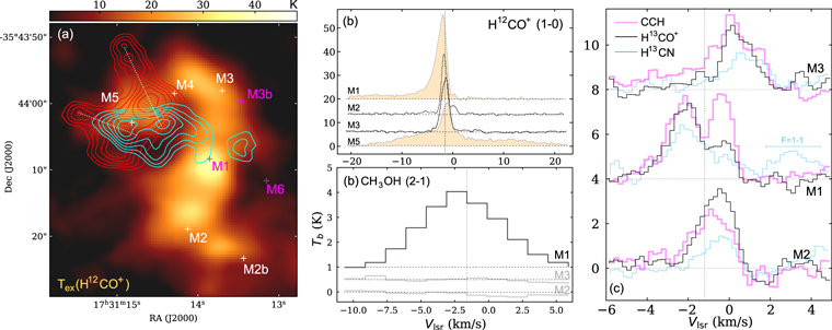
Figure 6. (a) The HCO+ outflow lobes overlaid on the HCO+ excitation temperature map. The line intensity is converted to Tex using Equation (A3). The contour levels are 15%–90% of the maximum intensity, which is 22.6 and 22.9 K km s−1 for the blue and red lobes, respectively. (b, c) The molecular spectra at selected cores. For each spectrum, the horizontal line represents the zero-level baseline. The vertical dashed line denotes the division between the blueshift gas (M1 core) and main-filament components.
Download figure:
Standard image High-resolution imageFrom the HCO+ line-wing intensities and outflow emission areas, the outflow lobes are found to have masses mblue = 0.20 M⊙ and mred = 0.24 M⊙. And the average radius is Rout = (8 ± 3)″ = (5.5 ± 2) × 103 au. Assuming an average velocity of vout = 8 km s−1, the outflow age is derived to be tout = Rout/vout = (3.5 ± 1) × 103 yr.