Abstract
LaO bands are a characteristic feature in the spectrum of cool S-type stars. La is made primarily by the s-process during the asymptotic giant branch phase of stellar evolution. The B2Σ+–X2Σ+ and A2Π–X2Σ+ band systems can be used to determine the La abundances in cool S stars. The bands of the B2Σ+–X2Σ+ with  and
and  have been rotationally analyzed from an emission spectrum from a carbon furnace. Line strengths are calculated using an ab initio transition dipole function, corrected using experimental lifetimes. We provide a line list for the B2Σ+–X2Σ+ band system that can be used to determine La abundances.
Original content from this work may be used under the terms of the Creative Commons Attribution 4.0 licence. Any further distribution of this work must maintain attribution to the author(s) and the title of the work, journal citation and DOI.
1. Introduction
The formation of the elements is an active area of research (Johnson 2019). For example, the important role of neutron star mergers in the synthesis of heavy elements has recently become evident (Ji et al. 2019). Lanthanum (La) is formed both in the rapid neutron-capture process (r-process) in kilonovae from neutron star mergers and in the slow neutron-capture process (s-process) in asymptotic giant branch (AGB) stars (Johnson 2019). The s-process is thought to be responsible for the synthesis of about half of the elements heavier than Fe (Neyskens et al. 2015). The s-process can be studied by measuring the stellar abundance of heavy elements such as Y, Zr, Ba, and La that are formed from lighter elements by the repeated absorption of a neutron followed by β-decay. For hot stars using atomic La+ ions (e.g., La ii 4921.778 Å) for abundance measurements is convenient, but for cooler objects, the visible and near-infrared electronic transitions of LaO are more useful (MacConnell et al. 2000).
The s-process takes place in the late AGB phase of stellar evolution when most of the hydrogen has been consumed (Wallerstein et al. 1997). Helium and hydrogen burning occur in thin shells around a C/O core and thermal pulses dredge up carbon and other elements. The stellar surface becomes increasingly rich in carbon, ultimately forming a carbon star. S stars have carbon abundances approximately equal to their oxygen abundances and display spectral features associated with s-process elements, e.g., LaO bands from the B2Σ+–X2Σ+ and A2Π–X2Σ+ transitions. LaO line lists are needed to determine La abundances in cool S-type stars. The goal of our work is to provide a modern line list for the B2Σ+–X2Σ+ band system of LaO for this purpose.
LaO has four low-lying electronic states: X2Σ+,  , A2Π, and B2Σ+. The green B2Σ+–X2Σ+ transition and the very red A2Π–X2Σ+ transition have been studied many times (Bacis et al. 1973; Bernard & Sibaï 1980; Bernard et al. 1999) and the A2Π–A
  emission bands can be seen near 2 μm in the near-infrared (Bernard & Vergès 2000). The rotational lines of the A–X and B–X electronic transitions are doubled with a splitting of about 0.5 cm−1. This unusual feature caused considerable confusion until Weltner et al. (1967) assigned the splitting to large magnetic hyperfine structure (hfs) in the X2Σ+ state due to the 139La nucleus. Childs et al. (1986) studied the hfs in the X2Σ+ and B2Σ+ states with great precision by laser-radio frequency double resonance in a molecular beam. Ground-state microwave spectroscopy has also been carried out (Törring et al. 1988; Suenram et al. 1990). Steimle & Virgo (2002) measured the dipole moments in the X2Σ+, A2Π, and B2Σ+ states and analyzed the hfs in the A2Π state.
Radiative lifetimes for the B2Σ+ state have been measured by laser-induced fluorescence (Liu & Parson 1977; Carette & Bencheikh 1994). Finally, there are several ab initio calculations of LaO molecular properties (Schamps et al. 1995; Moriyama et al. 2010; Korek et al. 2013).
We report a reanalysis of the B2Σ+–X2Σ+ band system up to v = 5 in both ground and excited states. Using an ab initio transition dipole moment function, scaled with experimental data, we have calculated the line strengths and provide a line list suitable for the simulation of stellar spectra.
2. Experiment
The emission spectrum of LaO was recorded in 1988 using a carbon tube furnace (King furnace) with the McMath-Pierce 1 m Fourier transform spectrometer at the National Solar Observatory at Kitt Peak in Arizona. The data are available from the National Solar Observatory Digital Library as file 881025-03. The furnace had a temperature of 2100°C. The spectrometer was operated with silicon diode detectors and covered the nominal range of 350–1100 nm set by the visible beamsplitter and the silicon diodes. Eight scans were recorded in about 1 hr at a spectral resolution of 0.05 cm−1.
An overview spectrum of the Δv = 1 sequence of the B2Σ+–X2Σ+ transition is provided in Figure 1. Figure 2 shows the spectrum near the 1–0 band heads. The calculation of the simulated spectra in the two figures is discussed below.
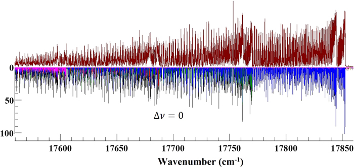
Figure 1. Overview emission spectrum of LaO (above) and simulation (below) of the Δv = 0 sequence of the B2Σ+–X2Σ+ transition. (Blue: 0–0 band, green: 1–1 band, red: 2–2 band, and pink: 3–3 band.)
Download figure:
Standard image High-resolution image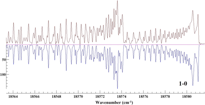
Figure 2. The spectrum of LaO (above) and simulation (below) of the B–X 1–0 band.
Download figure:
Standard image High-resolution image3. Ab Initio Calculations
The electric transition dipole moment (TDM) curve for the B2Σ+–X2Σ+ transition has been calculated using the MOLPRO Quantum Chemistry package (Werner et al. 2012, 2019). These calculations were performed with the internally contracted configuration interaction method (ic-MRCI; Knowles & Werner 1988; Werner & Knowles 1988), using molecular orbitals optimized by means of state-averaged complete active space self-consistent field (SA-CASSCF) calculations (Knowles & Werner 1985; Werner & Knowles 1985). The state averaging has been applied to the X2Σ+(A1),  (A1+A2), and B2Σ+(A1) states, sharing the same A1 symmetry of the C2v
subgroup used by MOLPRO. Davidson's correction for unlinked clusters (Langhoff & Davidson 1974), adapted to a relaxed reference (Werner et al. 2008), has been taken into account in the energy calculations. The active space contains five σ, three π, and one δ molecular orbitals, correlating to the lanthanum 6s, 6p, and 5d and oxygen 2p atomic orbitals. Seven electrons are distributed in all possible ways in this active space, according to the spatial and spin symmetries of the calculated states. A quasirelativistic Wood–Boring energy-adjusted electron core potential (ECP) has been used for describing the 46 core electrons (Kr + 4d10) of the lanthanum atom (Dolg et al. 1989). The corresponding spd basis set has been used (Dolg et al. 1989), augmented by an uncontracted set of three f Gaussian functions (Weigand et al. 2009). The scalar relativistic effects taken into account by the ECP are essential for describing a system containing a heavy element like lanthanum, as shown by the atomic and molecular test calculations provided in the above referenced papers. Dunning's aug-cc-pVQZ correlation-consistent basis set (Dunning 1989; Kendall et al. 1992) has been adopted for the oxygen atom. The term energy values, Te
, for the
(A1+A2), and B2Σ+(A1) states, sharing the same A1 symmetry of the C2v
subgroup used by MOLPRO. Davidson's correction for unlinked clusters (Langhoff & Davidson 1974), adapted to a relaxed reference (Werner et al. 2008), has been taken into account in the energy calculations. The active space contains five σ, three π, and one δ molecular orbitals, correlating to the lanthanum 6s, 6p, and 5d and oxygen 2p atomic orbitals. Seven electrons are distributed in all possible ways in this active space, according to the spatial and spin symmetries of the calculated states. A quasirelativistic Wood–Boring energy-adjusted electron core potential (ECP) has been used for describing the 46 core electrons (Kr + 4d10) of the lanthanum atom (Dolg et al. 1989). The corresponding spd basis set has been used (Dolg et al. 1989), augmented by an uncontracted set of three f Gaussian functions (Weigand et al. 2009). The scalar relativistic effects taken into account by the ECP are essential for describing a system containing a heavy element like lanthanum, as shown by the atomic and molecular test calculations provided in the above referenced papers. Dunning's aug-cc-pVQZ correlation-consistent basis set (Dunning 1989; Kendall et al. 1992) has been adopted for the oxygen atom. The term energy values, Te
, for the  and B states are calculated to be 8189 and 18,121 cm−1, respectively, in agreement with the corresponding experimental values of 7844.1 (Bernard & Vergès 2000) and 17,878.7 cm−1 (Bernard et al. 1999). The calculations have been carried out at a set of internuclear distances, R, ranging from 1.6 to 2.5 Å, by steps of 0.05 Å, and the resulting TDM curve has been interpolated by B-splines to create a set of 1592 points on the same R range. The calculated points and the interpolated points are provided as supplementary data. This curve is shown in Figure 3. The inflection point at 2.15 Å results from an interaction between the two higher π orbitals of the active space. This transition function has not been predicted in previous ab initio works.
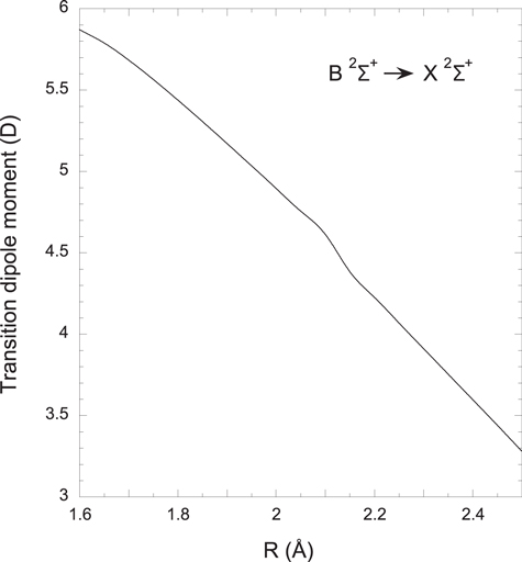
Figure 3. Ab initio transition dipole moment curve for the B2Σ+–X2Σ+ transition of LaO.(The data used to create this figure are available.)
Download figure:
Standard image High-resolution image4. Line Positions
The B2Σ+–X2Σ+ transition of LaO was rotationally analyzed using the PGOPHER program (Western 2017) with the experimental spectrum used as an overlay. The rotational structure of the LaO 2Σ+ states can be described by the standard N 2 Hamiltonian ( H rot), where N is the rotational angular momentum ( N = J − S ), J is the total angular momentum excluding nuclear spin, S is the total electron spin, B is the rotational constant, and D and H are the centrifugal distortion constants (Brown & Carrington 2003):

The spin–rotation (electron spin, molecular rotation) interaction of LaO is described by H sr, where γ is the spin–rotation constant, and γD is the centrifugal distortion correction:

139La has a nuclear spin (I) of 7/2 (100% natural abundance), and the interaction of nuclear spin with the total angular momentum ( J ) gives rise to the nuclear hfs F = J + I of LaO. This hfs can be modeled using the Frosh and Foley constants (Frosch & Foley 1952) and the Hamiltonian for the hfs ( H hfs) can be written as (Childs et al. 1986; Törring et al. 1988; Steimle & Virgo 2002; Brown & Carrington 2003)
in which b is the Fermi contact constant, c is the dipole–dipole interaction constant, CI is the nuclear spin–rotation interaction constant, and eqQ is the nuclear quadrupole coupling constant. The effective Hamiltonian ( H eff) for LaO 2Σ+ states is thus

In the upper state (B2Σ+), the spin S of the unpaired electron couples with the rotational angular momentum N ( J = N + S ) and spin–rotation constant is known to be negative, so J = N-1/2 (F2) lies higher and J = N+1/2 (F1) lies lower (S = 1/2 for a doublet state). The resulting J couples with the nuclear spin I (I = 0 for 16O) to form up to eight (2I+1) hyperfine levels ( F = J + I ) known as bβ J coupling (Bacis et al. 1973; Brown & Carrington 2003).
For the ground state (X2Σ+), the Fermi contact parameter b is larger than the spin–rotation interaction. Therefore, it is convenient to couple the nuclear spin I and the electron spin S to form an intermediate angular momentum G = I + S . All rotational levels then split into two components, G = 4, which lies higher, and G = 3, which lies lower. Each G level couples with rotational angular momentum N , which forms up to 2G+1 hyperfine levels. This type of coupling F = G + N is known as bβ S coupling (Bacis et al. 1973; Brown & Carrington 2003). The G = 4 to G = 3 splitting is about 0.52 cm−1 and is responsible for the unusual doubling of the lines.
The vibrational and rotational dependence of these interactions can be taken into account by expanding each quantity (Xi,j ) in a Dunham-type power series,

Using this expansion Childs et al. (1986) were able to determine the v dependence of the hfs and spin–rotation constants for both X2Σ+ and B2Σ+ states. Since their constants are more precise than can be obtained from our experiment, the hfs constants determined by Childs et al. (1986) were used in our analysis to calculate the constants up to v = 5 in both X2Σ+ and B2Σ+ states and were held fixed during the fitting. In addition, the spin–rotation constants of Childs et al. (1986) were used to calculate these parameters for the ground state. The calculated values are given in Tables 1 and 2.
Table 1. Spectroscopic Parameters for the X2Σ+ State
| v = 0 | v = 1 | v = 2 | v = 3 | v = 4 | v = 5 | |
|---|---|---|---|---|---|---|
| Tv | 0 a | 812.73754(70) | 1621.19342(72) | 2425.35172(82) | 3225.18499(94) | 4020.6780(12) |
| Bv | 0.351807477 a | 0.350377881 a | 0.348942339 a | 0.347500853 a | 0.346053423 a | 0.344600047 a |
| 107 Dv | 2.6246 a | 2.6224 a | 2.6201 a | 2.61788 a | 2.61561 a | 2.6133 a |
| 103 γv | 2.2081 b | 2.22181 b | 2.23685 b | 2.25321 b | 2.2709 b | 2.28992 b |
| 108 γDv | −1.45734 b | −1.43666 b | −1.41598 b | −1.3953 b | −1.3746 b | −1.3539 b |
| 1014 γHv | 4.4364 b | 4.4364 b | 4.4364 b | 4.4364 b | 4.4364 b | 4.4364 b |
| b | 0.121147 b | 0.121232 b | 0.121317 b | 0.121401 b | 0.1214860 b | 0.121571 b |
| 103 c | 3.1596 b | 3.18 b | 3.200 b | 3.2208 b | 3.2412 b | 3.2617 b |
| 103 eqQ | −2.8131 b | −2.807 b | −2.8017 b | −2.7961 b | −2.7904 b | −2.7847 b |
| 107 CI | 4.818 b | 4.818 b | 4.818 b | 4.818 b | 4.818 b | 4.818 b |
| 108 bD | 2.66851 b | 2.66851 b | 2.66851 b | 2.66851 b | 2.66851 b | 2.66851 b |
| 109 cD | 6.2543 b | 6.2543 b | 6.2543 b | 6.2543 b | 6.2543 b | 6.2543 b |
| 108 eqQD | −1.4777 b | −1.4777 b | −1.4777 b | −1.4777 b | −1.4777 b | −1.4777 b |
Notes. One standard deviation is given in parenthesis. All values are in cm−1.
a Held fixed during fitting. Values are from Dunham constants of Törring et al. (1988). b Held fixed during fitting. Values are from Childs et al. (1986).Download table as: ASCIITypeset image
Törring et al. (1988) have obtained a precise set of rotational constants for v = 0–2 of the X2Σ+ state by microwave spectroscopy. Bv and Dv for the X2Σ+ state vibrational levels up to v = 5 were calculated using Equations (6) and (7), and were fixed for the X2Σ+ state (Table 1):


Bernard et al. (1999) obtained equilibrium spectroscopic constants for both X2Σ+ and B2Σ+ states. We used the equilibrium constants from Bernard et al. (1999) to calculate the starting values for the origins of the X2Σ+ and B2Σ+ vibrational levels for v = 0 to v = 5. The initial values of Bv , Dv , and γv for the B2Σ+ state were also calculated from the spectroscopic constants given in Bernard et al. (1999). The final fitted values for the spectroscopic constants and all constants held fixed in the X2Σ+ and B2Σ+ states are given in Tables 1 and 2. The associated matrix elements for the Hamiltonian used in the fitting are available from PGOPHER (Western 2017).
Table 2. Spectroscopic Constants for the B2Σ+ State
| v = 0 | v = 1 | v = 2 | v = 3 | v = 4 | v = 5 | |
|---|---|---|---|---|---|---|
| Tv | 17837.3937(17) | 18567.6509(13) | 19293.8973(14) | 20016.1283(14) | 20734.2972(21) | 21448.3950(39) |
| Bv | 0.34055994(56) | 0.33902396(38) | 0.33748655(53) | 0.33594209(46) | 0.3343991(11) | 0.3328452(22) |
| 107 Dv | 2.93981(39) | 2.93253(23) | 2.92742(40) | 2.92026(33) | 2.9266(13) | 2.9182(25) |
| γv | −0.253556(35) | −0.253450(25) | −0.253252(30) | −0.253266(25) | −0.253778(31) | −0.253434(51) |
| 107 γDv | −2.674(40) | −2.624(26) | −2.666(39) | −2.390(33) | ... | ... |
| 102 b | 1.94 a | 1.905 a | 1.871 a | 1.837 a | 1.802 a | 1.768 a |
| 103 c | 6.409 a | 5.939 a | 5.469 a | 4.998 a | 4.528 a | 4.058 a |
| 103 eqQ | −6.56 a | −6.776 a | −6.993 a | −7.21 a | −7.43 a | −7.64 a |
Notes. One standard deviation is given in parentheses. All values are in cm−1.
a Held fixed during fitting. Values are from Childs et al. (1986).Download table as: ASCIITypeset image
In the analysis, 12,120 lines were assigned in the 2–0, 3–1, 4–2, 5–3, 1–0, 2–1, 3–2, 4–3, 5–4, 0–0, 1–1, 2–2, 3–3, 4–4, 5–5, 0–1, 1–2, 2–3, 3–4, 4–5, 0–2, 1–3, 2–4, and 3–5 bands. Maximum  values are 120.5, 131.5, 120.5, 125.5, 93.5, and 89.5 for
  = 0, 1, 2, 3, 4, and 5, respectively. A sample of the observed and calculated line list is given in Table 3. The labeling for the lines provided in Table 3 is
  , in which N is the quantum number for rotational angular momentum, J is the quantum number for total angular momentum exclusive of nuclear spin, and
  ,
,  , and F; subscripted Fi,j
are the customary labels for the two spin components of a 2Σ+ states, 1 has J = N + 1/2 and 2 has J = N − 1/2, and the trailing
, and F; subscripted Fi,j
are the customary labels for the two spin components of a 2Σ+ states, 1 has J = N + 1/2 and 2 has J = N − 1/2, and the trailing  and
and  values are the total angular momentum including nuclear spin. As usual, primes are for the upper B state, and double primes are for the lower X state.
Table 3. Sample of Observed and Calculated Line List of the B–X Transition

|

|

|

| Obs (cm−1) | Calc (cm−1) | Obs-Calc (cm−1) | Line Assignment |
|---|---|---|---|---|---|---|---|
| 55 | f | 54 | f | 17849.6052 | 17849.6233 | −0.0181 | rR2(50.5)55,54 : B v = 0 51.5 52 F2f 55—X v = 0 50.5 51 F2f 54 |
| 47 | e | 46 | e | 17849.6052 | 17849.5800 | 0.0252 | rR2(49.5)47,46 : B v = 0 50.5 51 F2f 47—X v = 0 49.5 50 F2f 46 |
| 54 | e | 53 | e | 17849.6052 | 17849.6214 | −0.0162 | rR2(50.5)54,53 : B v = 0 51.5 52 F2f 54—X v = 0 50.5 51 F2f 53 |
| 48 | f | 47 | f | 17849.6052 | 17849.5533 | 0.0519 | rR2(49.5)48,47 : B v = 0 50.5 51 F2f 48—X v = 0 49.5 50 F2f 47 |
| 53 | f | 52 | f | 17849.6052 | 17849.6187 | −0.0135 | rR2(50.5)53,52 : B v = 0 51.5 52 F2f 53—X v = 0 50.5 51 F2f 52 |
Note.
 and
and  are the total angular momentum of the B and X states, respectively. p is the parity. Obs is the observed line position in cm−1; Calc is the calculated line position in cm−1; Obs-Calc is the difference of observed and calculated line position in cm−1. Line assignment illustrates the transition
  : B v
: B v 
 F1p/F2p
 - X v
- X v 
 F1p/F2p
 .
.
Only a portion of this table is shown here to demonstrate its form and content. A machine-readable version of the full table is available.
Download table as: DataTypeset image
5. Line Strengths and Line Lists
The calculation of line strengths is based on the ab initio transition dipole moment and RKR potential curves. The inputs for Le Roy’s RKR program (Le Roy 2017a) are the customary Bv (Equation (6)) and Gv expressions:
The rotational constants and band origins in Tables 1 and 2 were fitted to determine the equilibrium constants in Table 4. The equilibrium rotational constants for the ground state are those of Törring et al. (1988). The two RKR potentials and the transition dipole moment functions were input into Le Roy’s LEVEL program (Le Roy 2017b), and the transition dipole matrix elements  for R(0) were calculated (Table 5) for all bands with
  and
and  . These values were used as the band strengths in PGOPHER. The line list was computed with PGOPHER for J < 200 (Table 6). Although the predicted line positions are increasing unreliable for J values beyond the maximum value observed, they provide opacity for low-resolution astronomical applications. The bond dissociation energy of LaO in the X2Σ+ state used in the LEVEL calculation was 782 ± 21 kJ mol−1 (65,370 cm−1; Darwent 1970).
Table 4. Equilibrium Constants of LaO for the X2Σ+ and B2Σ+ States a
| X2Σ+ | B2Σ+ | |
|---|---|---|
| ωe | 816.9969(25) | 734.2344(78) |
| ωe xe | 2.1243(11) | 1.9830(36) |
| 103 ωe ye | −3.48(13) | −4.09(45) |
| Be | 0.352520046 b | 0.3413261(17) |
| 103 αe | 1.42365 b | 1.5319(16) |
| 106 γe | −2.9724 b | −1.77(32) |
Notes.
a All values are in cm−1 b Held fixed during fitting. Values from Dunham constants of Törring et al. (1988).Download table as: ASCIITypeset image
Table 5. Band Strengths from LEVEL
 / /
| 0 | 1 | 2 | 3 | 4 | 5 |
|---|---|---|---|---|---|---|
| 0 | 4.94309 | 1.78918 | 0.505466 | 0.116356 | 2.25885 × 10⁻² | 3.34618 × 10⁻³ |
| 1 | −2.00225 | 4.18192 | 2.33711 | 0.8376475 | 0.226165 | 4.75155 × 10⁻² |
| 2 | 0.545388 | −2.64277 | 3.45503 | 2.62842 | 1.12914 | 0.341525 |
| 3 | −0.106461 | 0.923692 | −2.99886 | 2.76845 | 2.77356 | 1.38171 |
| 4 | 1.20215 × 10⁻² | −0.218389 | 1.27280 | −3.17634 | 2.13129 | 2.82974 |
| 5 | 1.1576 × 10⁻³ | 3.13752 × 10⁻² | −0.354142 | 1.59862 | −3.20517 | 1.55462 |
Note. These band strengths should be multiplied by a correction factor of 0.77. All values are in debye.
Download table as: ASCIITypeset image
Table 6. Sample Line List for the B–X Transition

|

| Position (cm−1) | Eup (cm−1) | Elow (cm−1) | A (s−1) | Line Assignment |
|---|---|---|---|---|---|---|
| 199 | 200 | 13451.4782 | 30773.5841 | 17322.1059 | 2.168176 | pP1(199.5)199,200 : B v = 0 198.5 198 F1e 199—X v = 5 199.5 199 F1e 200 |
| 200 | 200 | 13451.4882 | 30773.5941 | 17322.1059 | .0004978 | pP1(199.5)200,200 : B v = 0 198.5 198 F1e 200—X v = 5 199.5 199 F1e 200 |
| 198 | 199 | 13451.5029 | 30773.5744 | 17322.0715 | 2.013565 | pP1(199.5)198,199 : B v = 0 198.5 198 F1e 198—X v = 5 199.5 199 F1e 199 |
| 199 | 199 | 13451.5126 | 30773.5841 | 17322.0715 | .0005141 | pP1(199.5)199,199 : B v = 0 198.5 198 F1e 199—X v = 5 199.5 199 F1e 199 |
| 197 | 198 | 13451.5323 | 30773.5649 | 17322.0326 | 1.831155 | pP1(199.5)197,198 : B v = 0 198.5 198 F1e 197—X v = 5 199.5 199 F1e 198 |
| 198 | 198 | 13451.5418 | 30773.5744 | 17322.0326 | .0004662 | pP1(199.5)198,198 : B v = 0 198.5 198 F1e 198—X v = 5 199.5 199 F1e 198 |
| 196 | 197 | 13451.5689 | 30773.5558 | 17321.9869 | 1.598742 | pP1(199.5)196,197 : B v = 0 198.5 198 F1e 196—X v = 5 199.5 199 F1e 197 |
| 197 | 197 | 13451.5781 | 30773.5649 | 17321.9869 | .0003621 | pP1(199.5)197,197 : B v = 0 198.5 198 F1e 197—X v = 5 199.5 199 F1e 197 |
Note:
 and
and  are the total angular momentum of the B and X states, respectively. Position is the line position in cm−1. Eup and Elow are the energies of the B and X states in cm−1. Einstein A coefficients in s−1 are given under A. Line assignment illustrates the transition
  : B v
: B v 
 F1p/F2p
 - X v
- X v 
 F1p/F2p
 .
.
Only a portion of this table is shown here to demonstrate its form and content. A machine-readable version of the full table is available.
Download table as: DataTypeset image
The Einstein  (s−1) values were calculated using
  (Bernath 2020), where ν is the band origin for the B-X v′-v″ transition in cm−1 and
  is the transition moment (debye) given in Table 5, corrected by a factor of 0.77. The lifetime τ is calculated using all radiative rates connecting the upper vibrational level (
 ) to all lower vibrational levels (
 ):
):

The radiative lifetime of the B2Σ+ state is expected to be in the 20–40 ns range (Liu & Parson 1977), since LaO is isoelectronic to the alkaline earth monohalides for which lifetimes have been determined by Dagdigian et al. (1974). Liu & Parson (1977) have measured radiative lifetimes of 34.2 ± 1.5 ns and 35.5 ± 1.2 ns (at two wavelengths) for v = 0, and 36.0 ± 1.8 ns and 35.9 ± 2.4 ns for v = 1 in the B2Σ+ state by application of the laser-induced fluorescence technique. Later, Carette & Bencheikh (1994) determined the radiative lifetime of 32 ± 2 ns for the v = 0 B2Σ+ state. The calculated radiative lifetimes were low compared to the measurements carried out by Liu & Parson (1977) and Carette & Bencheikh (1994). Taking the average value to be 33.9 ± 2.8 ns for v = 0 compared to the calculated value of 20.13 ns for v = 0 suggests that a correction factor of 0.77 be applied to the transition dipole moments of Table 5. With this correction, the lifetimes we calculate are given in Table 7. This correction factor is not unreasonable considering the difficulty in calculating the properties of heavy elements, and strictly applies to the 0–0 band. Its application to other bands, particularly to off-diagonal bands, is an assumption.
Table 7. Radiative Lifetimes of LaO in B2Σ+
| B 2Σ+ v = | 0 | 1 | 2 | 3 | 4 |
|---|---|---|---|---|---|
| τn (ns) | 33.90 | 34.42 | 34.94 | 35.63 | 38.97 |
Download table as: ASCIITypeset image
6. Discussion
The energy levels for v = 0 to v = 5 for both the X2Σ+ and B2Σ+ states were determined. The origin determined by Bernard & Sibaï (1980) for v = 0 for the B2Σ+ state is 17,837.345(30) cm−1 and for v = 1 for the X2Σ+ and B2Σ+ states are 812.676(69) cm−1 and 18,567.613(69) cm−1, respectively. Our values (Tables 1 and 2) for the same vibrational levels are the same within error. X2Σ+ state equilibrium constants calculated by Bernard et al. (1999) are ωe = 817.0264(78) cm−1, ωe xe = 2.1292(24) cm−1, and ωe ye = −0.00315(24) cm−1. B2Σ+ state equilibrium constants calculated by Bernard et al. (1999) are ωe = 734.2811(87) cm−1, ωe xe = 1.9922(29) cm−1, and ωe ye =−0.00354(32) cm−1. Our analysis was done with six vibrational levels in both X2Σ+ and B2Σ+, and a three-parameter fit was selected as most reasonable. Our values are in satisfactory agreement with those of Bernard et al. (1999). Bernard et al. (1999) determined Be = 0.34133169(95) cm−1, and αe =0.00154227(34) cm−1 for the B2Σ+ state. These values agree with our analysis (Table 4). Higher J lines in the simulated spectrum are a little off from the observed spectrum and relatively few of the 5–5 band lines could be assigned. Overall the simulated spectrum matches the observed LaO B–X transition.
7. Conclusion
Spectroscopic constants for LaO were determined up to v = 5 in both the B2Σ+ and X2Σ+ states. Three-parameter equilibrium constants for X state and for the B state were calculated. These equilibrium constants were used to calculate RKR potentials. The RKR potentials were combined with an ab initio transition dipole moment function to calculate band strengths, which were corrected using experimental lifetimes. PGOPHER provided the final line list for the B2Σ+–X2Σ+ band system. The line list can be used to simulate LaO spectra of cool S stars to determine La abundances.
The National Solar Observatory (NSO) is operated by the Association of Universities for Research in Astronomy, Inc. (AURA), under cooperative agreement with National Science Foundation. Financial support was provided by the NASA Laboratory Astrophysics Program (80NSSC21K1463). J.L. thanks the Consortium des Équipements de Calcul Intensif (CÉCI), funded by the Fonds de la Recherche Scientifique de Belgique (F.R.S.-FNRS) under grant No. 2.5020.11 and by the Walloon Region, for computational resources.
Software: PGOPHER (Western 2017), RKR (Le Roy 2017a), LEVEL (Le Roy 2017b), Excel (Microsoft), Wolfram Mathematica.