Abstract
In this paper, we present two distinct types of coronal mass ejection (CME)-flare relationships according to their observing time differences using 107 events from 2010 to 2013. The observing time difference, ΔT, is defined as flare peak time minus CME first appearance time at Solar Terrestrial Relations Observatory (STEREO) COR1 field of view. There are 41 events for group A (ΔT < 0) and 66 events for group B (ΔT ≥ 0). We compare CME 3D parameters (speed and kinetic energy) based on multi-spacecraft data (SOlar and Heliospheric Observatory (SOHO) and STEREO A and B) and their associated flare properties (peak flux, fluence, and duration). Our main results are as follows. First, there are better relationships between CME and flare parameters for group B than that of group A. In particular, CME 3D kinetic energy for group B is well correlated with flare fluence with the correlation coefficient of 0.67, which is much stronger than that (cc = 0.31) of group A. Second, the events belonging to group A have short flare durations of less than 1 hr (mean = 21 minutes), while the events for group B have longer durations up to 4 hr (mean = 81 minutes). Third, the mean value of height at peak speed for group B is 4.05 Rs, which is noticeably higher than that of group A (1.89 Rs). This is well correlated with the CME acceleration duration (cc = 0.75). A higher height at peak speed and a longer acceleration duration of CME for group B could be explained by the fact that magnetic reconnections for group B continuously occur for a longer time than those for group A.
1. Introduction
Coronal mass ejections (CMEs) are one of the major eruptive phenomena of the Sun and emit a large amount of energy into the interplanetary space. In particular, front-side halo CMEs are main causes of heliospheric and geomagnetic disturbances (St. Cyr et al. 2000; Webb et al. 2000; Kim et al. 2005; Moon et al. 2005). It is well known that most of the halo CMEs are associated with major flares (Harrison 1995; Aarnio et al. 2011) and their eruption processes are relatively well explained by the standard CME-flare model (CSHKP; Carmichael 1964; Sturrock 1968; Hirayama 1974; Kopp & Pneuman 1976). Recently, the CME-triggering mechanism has been studied in terms of several perspectives: the tether-cutting (e.g., Moore et al. 2001), the break-out model (e.g., Antiochos et al. 1999), and the kink instability (e.g., Török & Kliem 2005).
For over two decades, there have been many studies on the comparison between CME properties observed by coronagraphs and its associated flare ones observed by Geostationary Operational Environmental Satellite (GOES). Using the 249 events observed by the Solar Maximum Mission (SMM), Hundhausen (1997) reported the relationship between CME kinetic energy and integrated soft X-ray (SXR) flux (i.e., fluence) with a correlation value of 0.53. According to results from Moon et al. (2002), there is a positive correlation (cc = 0.47) between speeds of limb CMEs observed by the Large Angle Spectroscopic Coronagraph (LASCO; Brueckner et al. 1995) on board the Solar and Heliospheric Observatory (SOHO; Domingo et al. 1995) and integrated SXR fluxes from 1996 and 2002. Burkepile et al. (2004) found that the correlation coefficient between CME kinetic energy and flare peak flux is 0.74 for 24 limb CMEs, which had both speed and mass measurements. Vršnak et al. (2005) also presented that the CME speed and width increase with flare strength. They introduced a proxy of CME kinetic energy, which is defined as a square of average speed multiplied by an angular width of CME, and found that the correlation between this proxy and integrated SXR flux is 0.47. Bein et al. (2012) reported a weak positive correlation between CME peak speed observed by the Solar Terrestrial Relations Observatory (STEREO; Kaiser et al. 2008) and flare peak flux (cc = 0.32). Summing up, the correlation value between CME speed (or kinetic energy) and flare strength (or fluence) ranges from 0.32 to 0.74, which depends on what considered CMEs are limb events or not. All of these results are based on the fact that CME properties are obtained by a single coronagraph.
In this paper, we want to make a new attempt to obtain better relationships between CMEs and flares with the following two perspectives. First, we use the three-dimensional (3D) parameters of CMEs to reduce the projection effect of CME properties. STEREO makes it possible to determine the CME 3D parameters (speed, width, etc.) by applying the stereoscopic method based on multi-view observations (Thernisien et al. 2009; Liu et al. 2010; Millward et al. 2013). According to quadratic observations between SOHO and STEREO, several researchers found that apparent angular widths observed from SOHO LASCO and STEREO COR2 are quite different from each other (Gopalswamy et al. 2012; Lee et al. 2015). Using 306 front-side halo (partial and full) CMEs from 2009 to 2013, Jang et al. (2016, hereafter Paper I) presented statistical comparison between CME projected two-dimensional (2D) parameters from single coronagraph (LASCO) and 3D ones from multi coronagraphs (STEREO A and B), which is calculated by the stereoscopic CME analysis tool (StereoCAT) provided by NASA Community Coordinated Modeling Center (CCMC). They found that projected speeds tend to be approximately 20% underestimated when compared with 3D speeds. They also found that the apparent angular width of a halo CME seen by SOHO is quite different from its 3D width, which ranges from  to
to  . Until now, there has been no comprehensive study on the comparison between CME 3D parameters and flare ones. Second, we use the data from COR1 of the Sun Earth Connection Coronal and Heliospheric Investigation (SECCHI; Howard et al. 2008) on board STEREO, which covers from 1.4 to 4 solar radii, to investigate the propagation of CMEs in low corona. It is hard to measure a CME start time using direct observations, because the low coronal region is hidden by occulters of coronagraphs. A typical method to estimate a CME start time is a height-time extrapolation with the assumption of a constant speed or acceleration (Zhang et al. 2002; Michalek 2009; Youssef et al. 2013). This is still not accurate because there are several phases of CME evolution with different speeds in the low corona (Zhang & Dere 2006). Here, we use COR1 data to directly determine the first appearance times and height-time measurements of CMEs. This can reduce the back-projection errors in height-time of CMEs observed in COR2.
In this paper, we make a comparison between CME 3D parameters from multi-spacecraft and its associated flares according to their observational time difference between flare peak time on X-ray flux and CME first appearance time at COR1. In Section 2, we explain our data set and observing time differences. Then our results and a discussion are presented in Section 3. A brief summary and conclusion are delivered in Section 4.
2. Data and Method
To compare between the CME 3D parameters and its associated flare ones, we use data taken from Paper I, which are 306 LASCO front-side halo CMEs (apparent angular width  ) from 2009 to 2013. These CMEs are well observed by both SOHO and STEREO A and B and their structures are clearly seen in more than two coronagraph data among the three spacecraft.
Among 306 events, we choose 107 flare-associated CMEs with the following criteria. (1) We pick flares that start within 2 hr of the CME first observing times in LASCO C2 in order to select a flare closely related to CME. (2) We try to find the change of the loop in the Atmospheric Imaging Assembly (AIA; Lemen et al. 2012)  , on board Solar Dynamics Observatory (SDO), or filament eruption in AIA
  near the flaring region in the same sector of CME occurrence during a 2 hr time window. For the same event, we reconfirm the association using additional data set such as Extreme Ultraviolet Imager (EUVI; Wuelser et al. 2004)
  ,
,  , COR1, and COR2 of STEREO A or B. (3) If there are several flares during the time window, we carefully inspect the evolution of SDO and coronagraph images and determine the corresponding flare, which all correspond to the largest flares. (4) Only flares observed within ±70° longitude of solar central meridian as seen by SDO AIA are considered. To check out whether this method is reasonable, we plot the histogram of the separation angle between measurement position angle (MPACME) and the position angle of flare location (PAflare) as shown in Figure 1. Most of the events are spatially well consistent with each other. It is also noted that the events with large separation angle occur near the solar center.
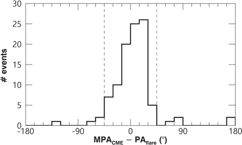
Figure 1. Histogram of the separation angle between measurement position angle (MPACME) and the position angle of flare location (PAflare). The dashed lines indicate that the angle is ±45°.
Download figure:
Standard image High-resolution imageTo estimate CME 3D speed, we use the StereoCAT (see Mays et al. 2015, and references therein)4 based on a triangulation method, which is provided by CCMC at NASA. More detailed descriptions about CME 3D parameters are given in Paper I. These CMEs have two-dimensional (2D) parameters, which correspond to projected values obtained from single spacecraft (SOHO LASCO). The projected speed (2D speed) and mass are directly taken from SOHO LASCO CME catalog (Yashiro et al. 2004).5 Flare parameters (peak flux, fluence, and duration) are taken from National Geophysical Data Center (NGDC) flare list.6 The events we used are 14 X-class flares, 44 M-class flares, 44 C-class flares, and 5 B-class flares.
In this study, we use the CME first appearance time using STEREO COR1, which can observe low corona between 1.4 and 4 Rs (Howard et al. 2008). Besides, it has a high time cadence of 2.5 minutes (sometimes 5 minutes). Here we define the observing time difference, ΔT, as flare peak time minus CME first appearance time. According to this observing time difference, we divide the data into two different groups. A negative value of time difference (ΔT < 0), called group A, indicates that a CME first appears in the COR1 field of view after its associated flare peak time. Whereas, a positive value (ΔT  0), called group B, implies that a CME first appears before the flare peak time. Figure 2 shows a histogram of the time differences for 107 events. Among them, there are 41 events for group A and 66 events for group B. This histogram approximately follows a normal distribution, with mean and median values of 6.5 and 3 minutes, respectively.
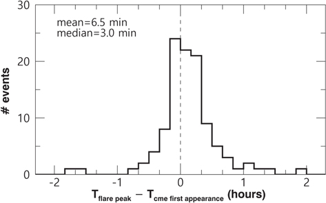
Figure 2. Histogram of observing time differences between flare peak time and CME first appearance time in the STEREO COR1 field of view. Mean and median values are 6.5 and 3 minutes, respectively. The vertical dashed line indicates that the time difference is zero.
Download figure:
Standard image High-resolution image3. Result and Discussion
We compare CME 2D and 3D parameters, such as speed and kinetic energy, with parameters of their associated flares. Although all CME parameters have relationships with two flare parameters (peak flux and fluence), there are better correlations of CME parameters with fluence than those with peak flux. Hereafter we show relationships of CME parameters and fluence.
Figure 3 shows a comparison between CME speeds and flare fluences. A correlation coefficient (0.53) between the 3D speed (V3D) and the fluence for all events is slightly higher than that (0.49) between the 2D speed (V2D) and the fluence. These coefficients are somewhat higher than the results of Moon et al. (2002), who showed a correlation coefficient (0.47) between the 2D speed and the flare fluence for the limb events observed from 1996 to 2000. Our results are smaller than Salas-Matamoros & Klein (2015) who found that the correlation coefficient is 0.58 using 49 limb CMEs observed from 1996 to 2008. It is noted that the linear relationship (cc = 0.59) between the 3D speed and the fluence for group B is much clearer than that (cc = 0.32) for group A, which is also seen in the case of 2D speed. These kinds of low correlation coefficients of group A do not support a strong physical association between two parameters.
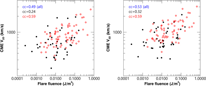
Figure 3. Relationship between CME speed and flare fluence: 2D (left) and 3D speed (right). Black closed and red open circles indicate results for groups A and B, respectively. The correlation coefficients for both groups are given in the Table 1.
Download figure:
Standard image High-resolution imageWe compare CME kinetic energy and flare fluence in Figure 4. The CME 2D speed is used to calculate 2D kinetic energy (E2D), and similarly 3D kinetic energy (E3D) comes from 3D speed. Because all the events are halo CMEs seen by LASCO, masses of CMEs measured by LASCO may have large uncertainties. Vourlidas et al. (2000) mentioned that LASCO measurements tend to underestimate the CME mass by about 50%. The uncertainties of CME speeds are about 10% as described in Paper I. Therefore, uncertainties of CME kinetic energies are mainly due to the mass underestimation. We find that correlation coefficients between CME kinetic energy and flare fluence for all events are 0.55 and 0.58 for 2D and 3D, respectively. These values are quite similar to result from Yashiro & Gopalswamy (2009) who found that the correlation between CME 2D kinetic energy and fluence is 0.56 using CMEs observed from 1996 to 2007. In particular, the correlation coefficient between 3D kinetic energy and flare fluence for group B is 0.67, which is much higher than that (0.39) for group A. This kind of noticeable difference between two groups is also seen in the 2D case.
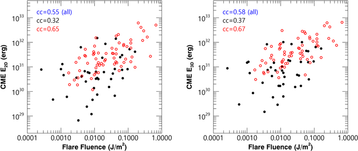
Figure 4. Relationship between CME kinetic energy and flare fluence: 2D (left) and 3D kinetic energies (right). Black closed and red open circles indicate results for groups A and B, respectively. The correlation coefficients for both groups are given in Table 1.
Download figure:
Standard image High-resolution imageWe summarize the correlation coefficients between CME and flare parameters, and their p-values in Table 1. The p-value means a probability to occur by chance when both quantities are randomly distributed, which depends on correlation coefficient and the number of data. Commonly, p-value <0.05 means that this relationship is statistically significant. All CME parameters have meaningful relationships with two flare parameters (peak flux and fluence), since all corresponding p-values are smaller than 0.05. It is noted that correlations of CME parameters with flare fluence for all events are quite higher than those with flare peak flux. For example, the correlation coefficient (cc = 0.58) of CME 3D kinetic energy with fluence is noticeably larger than that (cc = 0.30) with flux. This tendency is also found for the other CME parameters as well. This fact implies that flare fluence might be a better proxy for flaring energy than flare peak flux since it is an integration of GOES flux from flare starting time to end time (Krucker & Benz 1998; Veronig et al. 2002). According to previous studies (Yashiro & Gopalswamy 2009; Salas-Matamoros & Klein 2015), it is also found that a correlation coefficient of CME parameter (speed or kinetic energy) with flare fluence is a little higher than that with flare peak flux. In this study, we find that the correlations of 3D CME parameters with flare fluence, are equal to or a little higher than those of 2D values. In particular, it is noted that there are much better correlations between CME and flare parameters for group B than those for group A. The corresponding p-values for group B are all smaller than 0.001, which means that all these relationships are statistically significant. On the other hands, the p-values for group A are much greater than those for group B, and one p-value is larger than 0.05, which implies statistically insignificant.
Table 1. Correlation Coefficients between CME and Flare Parameters, and Their p-values
| V2D | V3D | E2D | E3D | |||
|---|---|---|---|---|---|---|
| All | cc | 0.29 | 0.30 | 0.30 | 0.30 | |
| p-value | 0.002 | 0.001 | 0.002 | 0.001 | ||
| Group A | cc | 0.16 | 0.22 | 0.28 | 0.32 | |
| Peak Flux | p-value | 0.306 | 0.171 | 0.075 | 0.041 | |
| Group B | cc | 0.51 | 0.54 | 0.56 | 0.58 | |
| p-value | <0.001 | <0.001 | <0.001 | <0.001 | ||
| All | cc | 0.49 | 0.53 | 0.55 | 0.58 | |
| p-value | <0.001 | <0.001 | <0.001 | <0.001 | ||
| Group A | cc | 0.24 | 0.32 | 0.32 | 0.37 | |
| Fluence | p-value | 0.128 | 0.043 | 0.038 | 0.015 | |
| Group B | cc | 0.59 | 0.59 | 0.65 | 0.67 | |
| p-value | <0.001 | <0.001 | <0.001 | <0.001 | ||
Download table as: ASCIITypeset image
Another flare parameter we investigate is the flare durations (Tflare) of the events. Tflare is defined as a time interval from flare start to end time. Tflare for group A are all less than 1 hr, which ranges from 6 and 53 minutes with a mean of 21 minutes. While Tflare for group B vary from 10 minutes to up to 4 hr with a mean of 81 minutes. Long duration flares ( hr) only occur in group B. We make a comparison between CME 3D kinetic energy and Tflare shown in Figure 5. We find that CME 3D kinetic energy tends to increase with its associated Tflare. Their correlation coefficient is 0.42 and its p-value is less than 0.05. There are events for only group B with high 3D kinetic energy bigger than approximately 1 × 1032 erg, while events with small kinetic energy less than 2 × 1030 erg belongs to only group A.
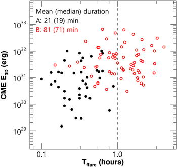
Figure 5. CME 3D kinetic energy plotted against flare duration. The vertical dashed line indicates the flare duration as 1 hr.
Download figure:
Standard image High-resolution imageWe carefully make a comparison between CME speed and GOES X-ray flux profiles. In order to obtain height-time measurements, we use STEREO EUVI 195 Å, COR1, and COR2. Here the height corresponds to a distance from solar center to the CME leading edge. When we measure heights of CME leading edges, we try to do three to five times in order to reduce the measurement errors and the uncertainties of heights are less than 10%. In order to minimize the projection effects, we select STEREO limb CMEs (31 events), whose source longitudes larger than  in the view of STEREO. There are 9 events for group A and 22 events for group B. Figure 6 shows a comparison between the height at CME peak speed, Hvpeak, and two types of durations: its associated flare duration, Tflare, and CME acceleration duration, Tacc. Tacc is assumed to be a time interval from the flare start time to the time at CME peak speed, because the CME initial acceleration phase is synchronized with flare rise phase (Zhang et al. 2001). We find that Tacc is very similar to flare rise time with a high correlation coefficient of 0.89.
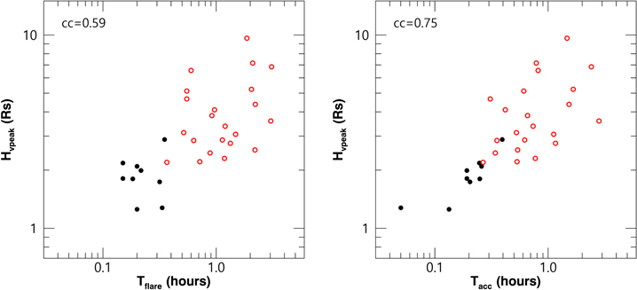
Figure 6. CME peak speed heights of limb CMEs shown as a function of flare duration (left) and CME acceleration duration (right). The CME acceleration duration is defined as CME peak speed time minus flare start time. Black closed circles correspond to results of group A and red open circles to those of group B.
Download figure:
Standard image High-resolution imageHvpeak of 31 CMEs range from 1.25 to 9.62 Rs with the mean of 3.42 solar radii. There is a general trend that Hvpeak increases with Tflare and Tacc with correlation coefficients of 0.59 and 0.75. The CMEs for group B have higher Hvpeak and longer Tacc than those of group A. The mean value of Hvpeak for group B is 4.05 Rs, which is noticeably higher than that (1.89 Rs) of group A. This means that CMEs for group B are more accelerated until higher Hvpeak than those for group A.
To show more quantitatively the characteristics of two groups, we select two representative events: 2011 September 7 event for group A and 2013 May 15 event for group B (Figure 7). These two events have similar flare strengths (X1.8 for group A event and X1.2 for group B event); however, CME 3D speeds are quite different; 751 km s−1 for group A event and 1667 km s−1 for group B event. The CMEs for both groups A and B are accelerated during the flare rise phase. The flare rise time of the first event is 12 minutes, while that of the latter event is 22 minutes. Hvpeak of the second one is 4.05 Rs, which is much higher than that (1.85 Rs) of the first one. A closer comparison between CME speed and GOES X-ray flux profile for two representative examples shows that the temporal evolutions of two profiles for group B are consistent with each other for a longer time than that for group A.
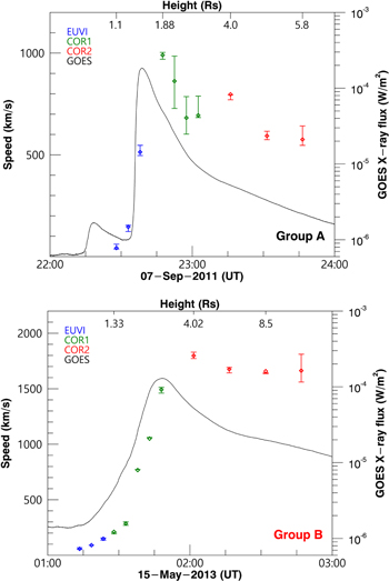
Figure 7. Comparison between GOES X-ray flux and CME speed profiles of two representative examples: 2011 September 7 event (top) for group A and 2013 May 15 event (bottom) for group B. Diamond symbols indicate the CME speed at a given time, which were estimated by a set of STEREO EUVI (blue), COR1 (green), and COR2 (red). Speeds are derived using the height difference between two successive data points obtained by the same instrument (e.g., EUVI or coronagraph). The error bars correspond to the minimum and maximum values of several measurements. The black lines indicate temporal profiles of GOES X-ray fluxes for two X-class flares.
Download figure:
Standard image High-resolution image4. Summary and Conclusion
We have investigated the CME-flare relationships using 107 halo CMEs from 2010 to 2013 observed by both SOHO and STEREO. To reduce the projection effects, we used the CME 3D parameters calculated by the stereoscopic CME analysis tool (StereoCAT). Then we examined the CME-flare relationship for all of the events as well as for two distinct groups according to their observing time difference (ΔT). A CME for group A appears in the COR1 field of view (ΔT < 0) after its associated flare peak time, while a CME for group B appears before flare peak time (ΔT  0). We have found that there are much higher correlation coefficients between CME parameters (speed and kinetic energy) and flare fluence for group B than those of group A. The most representative case is that CME 3D kinetic energy for group B is well correlated with flare fluence (cc = 0.67), which is much stronger than that (cc = 0.31) of group A. We also summarized the characteristics of CMEs and flares depending on two distinct groups (Table 2). For all events, mean values of CME 3D speed and kinetic energy are 1041 km s−1 and
  erg, respectively. Their associated Tflare is 58 minutes on average. We found that events for group B have larger values of CME and flare parameters than those of group A. The CMEs for group B have a higher mean speed (1182 km s−1), which is noticeably larger than that (814 km s−1) for group A. The mean 3D kinetic energy for group B is about 9 × 1031 erg, which is approximately five times higher than that for group A. The mean Hvpeak (4.05 Rs) for group B is much higher than that (1.85 Rs) for group A. Similarly, flares for group B have a much longer duration and rise time, which are about three times longer than those of group A.
Table 2. Mean (Median) Values of CME and Flare Parameters for all Events as well as two Distinct Groups
| Parameters | All | Group A | Group B |
|---|---|---|---|
| CME 3D speed | 1041 (916) km s−1 | 814 (683) km s−1 | 1182 (1079) km s−1 |
| CME 3D kinetic energy |
 ( ( ) erg ) erg |
 ( ( ) erg ) erg |
 ( ( ) erg ) erg |
| CME height at peak speeda | 3.47 (2.86) Rs | 1.85 (1.81) Rs | 4.05 (3.59) Rs |
| Flare duration | 58 (38) minutes | 21 (19) minutes | 81 (71) minutes |
| Flare rise time | 30 (22) minutes | 11 (9) minutes | 41 (31) minutes |
Note.
a31 limb CMEs seen by STEREO A or B.Download table as: ASCIITypeset image
The intimate relationship between flares and CMEs have been well observed and discussed by several studies (Zhang & Dere 2006; Maričič et al. 2007; Temmer et al. 2010), which insisted that there is a feedback relationship between CME initial acceleration and the flare energy release. According to the conventional CME-flare standard models (Shibata 1996; Lin & Forbes 2000), a current sheet is formed below the plasma bubble (i.e., CME) and a magnetic reconnection occurs in the vertical current sheet, which can be stretched by a rising motion of CME. Qiu et al. (2004) found that the total reconnection fluxes from flare observations are related to the CME speeds. Unfortunately, it is hard to directly observe the current sheets associated with flares. The post-CME current sheets have been only reported by several authors (Ko et al. 2003; Raymond et al. 2003; Webb et al. 2003; Bemporad 2008). Based on our results (Tables 1 and 2), faster CMEs associated with strong flares for group B tend to have a higher Hvpeak and a longer Tflare. It is very interesting to note that Hvpeak is well correlated with Tflare and Tacc. This fact implies that Hvpeak should be a proxy of the length of the current sheet in CME evolution. The CMEs with a higher Hvpeak and a longer Tacc for group B could indicate that magnetic reconnections for group B continuously occur for a longer time than those for group A. These results show that the CMEs for group B are more closely related to flares than those for group A.
This work was supported by the BK21 plus program through the National Research Foundation (NRF) funded by the Ministry of Education of Korea, the Korea Astronomy and Space Science Institute under the R&D program supervised by the Ministry of Science, ICT and Future Planning, Basic Science Research Program through the NRF funded by the Ministry of Education (NRF-2016R1A2B4013131), and NRF of Korea Grant funded by the Korean Government (NRF-2013M1A3A3A02042232). The SOHO/LASCO CME catalog (http://cdaw.gsfc.nasa.gov/CME_list/) is generated and maintained at the CDAW Data Center by NASA and the Catholic University of America in cooperation with the Naval Research Laboratory. SOHO is a project of international cooperation between ESA and NASA. The STEREO/SECCHI data are produced by an international consortium of the NRL, LMSAL and NASA GSFC (USA), RAL and University of Birmingham (UK), MPS (Germany), CSL (Belgium), IOTA, and IAS (France).
Footnotes
- 4
- 5
- 6