Abstract
Gas-phase molecules in cometary atmospheres (comae) originate primarily from (1) outgassing by the nucleus, (2) sublimation of icy grains in the near-nucleus coma, and (3) coma (photo)chemical processes. However, the majority of cometary gases observed at radio wavelengths have yet to be mapped, so their production/release mechanisms remain uncertain. Here we present observations of six molecular species toward comet 46P/Wirtanen, obtained using the Atacama Large Millimeter/submillimeter Array during the comet’s unusually close (∼0.1 au) approach to Earth in 2018 December. Interferometric maps of HCN, CH3OH, CH3CN, H2CO, CS, and HNC were obtained at an unprecedented sky-projected spatial resolution of up to 25 km, enabling the nucleus and coma sources of these molecules to be accurately quantified. The HCN, CH3OH, and CH3CN spatial distributions are consistent with production by direct outgassing from (or very close to) the nucleus, with a significant proportion of the observed CH3OH originating from sublimation of icy grains in the near-nucleus coma (at a scale length Lp = 36 ± 7 km). On the other hand, H2CO, CS, and HNC originate primarily from distributed coma sources (with Lp values in the range 550–16,000 km), the identities of which remain to be established. The HCN, CH3OH, and HNC abundances in 46P are consistent with the average values previously observed in comets, whereas the H2CO, CH3CN, and CS abundances are relatively low.
Original content from this work may be used under the terms of the Creative Commons Attribution 4.0 licence. Any further distribution of this work must maintain attribution to the author(s) and the title of the work, journal citation and DOI.
1. Introduction
Measurements of cometary compositions provide a unique tool for investigating ice chemistry in the protosolar disk midplane during the epoch of planet formation and can therefore provide insight into the reagents available for prebiotic chemistry in the early solar system (Mumma & Charnley 2011). A wealth of molecular species were recently detected in comet 67P by the Rosetta spacecraft (Altwegg et al. 2019), yet remote observations of coma gases remain the most common method for determining cometary compositions (Cochran et al. 2015).
The coma is typically understood in terms of a quasi-spherical expanding outflow of “parent” species sublimating directly from the nucleus, with “daughter” species originating from photolysis of the parents in the coma (Haser 1957). Several coma molecules, on the other hand, exhibit “distributed” (spatially extended) sources, some of which are believed to arise from the breakdown of macromolecular or dust grain precursors (Meier et al. 1993; Cottin & Fray 2008; Cordiner et al. 2014, 2017b), the precise identity of which remains unknown but could be related to the organic-rich refractory material identified in comet 67P by the Rosetta mission (Capaccioni et al. 2015; Fray et al. 2016; Bardyn et al. 2017). An analysis of a sample of 26 comets led Mumma et al. (2017) to propose that thermal dissociation of ammonium salts (NH4 +X−, where X− is a deprotonated acid) could be another source of gas-phase coma molecules, and this was found to be a plausible explanation for the abundances of several organics observed in the coma of 67P (Altwegg et al. 2020; Poch et al. 2020).
To date, interferometric observations using the Atacama Large Millimeter/submillimeter Array (ALMA) have confirmed the presence of daughter (or distributed) sources of H2CO in three comets, while the HNC and CS molecules have been found to exhibit distributed sources in two comets (Cordiner et al. 2014; Roth et al. 2021a; Biver et al. 2022). Earlier single-dish mapping work (Biver et al. 1999) and interferometric observations (Milam et al. 2006) identified extended H2CO spatial distributions in comets C/1996 B2 (Hyakutake) and C/1995 O1 (Hale–Bopp), respectively. Infrared spectroscopic studies have also indicated the presence of both nucleus and coma sources for H2CO and CO (Disanti et al. 1999; DiSanti et al. 2006), although no compelling evidence for a distributed CO source was found by Bockelée-Morvan et al. (2010). Despite decades of investigations into the chemical compositions of cometary comae and nuclei, it is surprising that the chemical origins of these commonly detected (and relatively simple) coma gases still remain to be conclusively determined.
A common way to parameterize molecular production in comets as a function of distance from the nucleus is using the Haser daughter formula (Haser 1957). Through radiative transfer modeling of coma mapping observations, it is possible to derive the characteristic distance scale at which a given species is produced (commonly expressed as a production scale length, or parent scale length, Lp ; Biver et al. 1999; Cordiner et al. 2014; Roth et al. 2021b). Due to the paucity of detailed studies to date and relatively large uncertainties on the derived Lp values for HNC, H2CO, and CS, combined with strong variability in the H2CO parent scale lengths derived for different comets (even after correcting for heliocentric distance), further studies are needed to help improve our understanding of the distributions of these molecules in cometary comae. By comparison with laboratory measurements and detailed numerical models (e.g., Meier et al. 1993; Fray et al. 2006; Cordiner & Charnley 2021), observational characterization of molecular production as a function of distance from the nucleus allows proposed identities of the parent species to be tested and validated. Measurements of the parent scale lengths of coma daughter species are therefore important in our quest to better understand the native chemical constituents of comets, from which we gain new insights into the chemical processes that occurred during the earliest history of the solar system.
Previous interferometric studies of molecular production scales in comets have been restricted to bright, long-period comets from the Oort cloud. But these objects represent only part of the wider population of small icy bodies available for study in our solar system today. Gravitational scattering by the giant planets is believed to have redistributed comets within the inner solar system and into their various present-day reservoirs, in particular, the Oort cloud and the Kuiper Belt or scattered disk. Most comets discovered each year come from the Oort cloud, while the scattered Kuiper disk is considered to be the source of Jupiter-family comets (JFCs). However, dynamical models have various predictions regarding the formative regions of comets, spanning a diverse range of heliocentric distances (e.g., Gomes et al. 2005; Tsiganis et al. 2005). It is therefore vitally important to study both Oort cloud comets (OCCs) and JFCs because it is unclear whether comets from each reservoir were formed in entirely overlapping regions in the protosolar disk. Comparative studies of JFCs and OCCs can also provide insights into the impact of solar irradiation and thermal processing on the nucleus composition, since JFCs are typically subject to repeated cycles of irradiation, heating, and cooling during their relatively frequent periodic perihelion passages (Meech & Svoren 2004; Gkotsinas et al. 2022). Due to its extremely close approach to Earth (Δ = 0.077 au on UT 2018 December 16), the 2018 apparition of comet 46P/Wirtanen provided a unique opportunity to observe the molecular coma of a JFC at unprecedented spatial resolution from the ground (henceforth, all dates refer to 2018 except where specified otherwise).
In this study, we present ALMA observations of molecular emission from comet 46P/Wirtanen conducted in early December, just before its closest approach to Earth. The resulting spectral images include molecules previously identified as daughter/distributed species in OCCs (H2CO, HNC, and CS), as well as suspected parent species (HCN and CH3OH). We also present the first map of CH3CN, which is yet to be imaged in any comet, so its association with sublimating ices in the nucleus or chemistry in the coma remains unexplored. Through application of our recently developed 3D radiative transfer and excitation model (SUBLIME; Cordiner et al. 2022), the coma temperature distribution is derived and parent scale lengths and abundances are calculated, leading to new insights into the nucleus-versus-coma contributions of the observed molecules.
2. Observations
ALMA observations of 46P/Wirtanen were carried out on UT December 2 and December 7, when the comet was ≈0.1 au from Earth (1.1 au from the Sun), using 43 12 m antennas in an intermediate array configuration (with baselines in the range 15–952 m; see Table 1). The comet was tracked, and the position of the array phase center on the sky was updated in real time using JPL Horizons orbital solution #K181/6. Weather conditions were very good throughout, with a vertical precipitable water vapor (PWV) column of less than 1 mm. This resulted in good phase stability, which was checked and corrected for with regular visits (every 6–7 minutes) to the nearby phase-calibration quasar J0241−0815.
Table 1. Observational Parameters
| Set. | UT Date | UT Time | Int. a | rH b | Δ c |
 d
d
| νR e | Band f | Baselines g |
 h
h
| θPB i | PWV j | ϕSTO k | Pos. Ang. l |
|---|---|---|---|---|---|---|---|---|---|---|---|---|---|---|
| (minutes) | (au) | (au) | (km s−1) | (GHz) | (m) | (arcsec) | (arcsec) | (mm) | (deg) | (deg) | ||||
| 1 | 2018 Dec 2 | 04:16–05:12 | 43 | 1.07 | 0.115 | −7.2 | 354.5 | 7 | 15.1–952 | 0.45 × 0.31 | 16.4 | 0.63 | 44.1 | 36.3 |
| 2 | 2018 Dec 2 | 02:30–03:52 | 63 | 1.07 | 0.115 | −7.4 | 351.8 | 7 | 15.1–952 | 0.41 × 0.31 | 16.5 | 0.90 | 44.2 | 36.2 |
| 3 | 2018 Dec 7 | 02:34–04:06 | 63 | 1.06 | 0.096 | −5.9 | 241.8 | 6 | 15.1–784 | 0.62 × 0.55 | 24.0 | 0.78 | 42.2 | 38.5 |
Notes.
a On-source observing time. b Heliocentric distance of the comet. c Geocentric distance of the comet. d Comet’s mean topocentric radial velocity. e Representative frequency. f The ALMA receiver band 6 range is 211–275 GHz; band 7 covers 275–370 GHz. g Range of antenna baseline lengths. h Angular resolution (dimensions of Gaussian fit to PSF) at νR . i Primary beam FWHM at νR . j Median PWV column length at zenith. k Sun–target–observer (phase) angle. l Position angle (in the plane of the sky) of the extended Sun–target vector, counterclockwise from north.Download table as: ASCIITypeset image
The ALMA correlator was configured to observe three spectral setups in receiver bands 6 and 7 covering lines from HCN (setting 1), HNC and H2CO (setting 2), and CH3OH, CH3CN, and CS (setting 3) with spectral resolutions in the range 122–977 kHz (0.1–1.1 km s−1). Integration times on source and other observational parameters are given in Table 1, while the detected spectral line frequencies of interest to the present study are shown in Table 2.
Table 2. Observed Spectral Line Parameters
| Species | Transition | Freq. | Eu | Res. |
|---|---|---|---|---|
| (MHz) | (K) | (kHz) | ||
| CH3OH | 50–40 E | 241,700.1590(0040) | 48 | 244 |
| CH3OH | 5−1–4−1 E | 241,767.2340(0040) | 40 | 244 |
| CH3OH | 50–40 A+ | 241,791.3520(0040) | 35 | 244 |
| CH3OH | 54–44 A± | 241,806.5240(0040) | 115 | 244 |
| CH3OH | 5−4–4−4 E | 241,813.2550(0040) | 123 | 244 |
| CH3OH | 53–43 A± | 241,833.1060(0040) | 85 | 244 |
| CH3OH | 52–42 A− | 241,842.2840(0040) | 73 | 244 |
| CH3OH | 53–43 E | 241,843.6040(0040) | 83 | 244 |
| CH3OH | 5−3–4−3 E | 241,852.2990(0040) | 98 | 244 |
| CH3OH | 51–41 E | 241,879.0250(0040) | 56 | 244 |
| CH3OH | 52–42 A+ | 241,887.6740(0040) | 73 | 244 |
| CH3OH | 5−2–4−2 E | 241,904.1470(0040) | 61 | 244 |
| CH3OH | 52–42 E | 241,904.6430(0040) | 57 | 244 |
| CS | 5–4 | 244,935.5565(0028) | 35 | 488 |
| CH3CN | 144–134 | 257,448.1282(0002) | 207 | 977 |
| CH3CN | 143–13−3 | 257,482.7919(0002) | 157 | 977 |
| CH3CN | 14−3–133 | 257,482.7919(0002) | 157 | 977 |
| CH3CN | 142–132 | 257,507.5619(0002) | 121 | 977 |
| CH3CN | 141–131 | 257,522.4279(0002) | 100 | 977 |
| CH3CN | 140–130 | 257,527.3839(0002) | 93 | 977 |
| H2CO | 51,5–41,4 | 351,768.6450(0300) | 62 | 244 |
| HCN | 4–3 | 354,505.4773(0005) | 43 | 122 |
| HNC | 4–3 | 362,630.3030(0090) | 44 | 244 |
Notes. All spectral line data were obtained from the Cologne Database for Molecular Spectroscopy (Endres et al. 2016). Transition quantum numbers are  –J″K″ for CH3OH and CH3CN,
  –
– for H2CO, and
  –J″ for CS, HCN, and HNC. Uncertainties on the trailing digits of the spectral line frequencies are given in parentheses.
Download table as: ASCIITypeset image
Noisy outlier data points were identified and flagged (removed) through inspection by Joint ALMA Observatory (JAO) staff. The raw data (visibilities) were further flagged and calibrated using the CASA software (version 5.4; CASA Team et al. 2022), using standard scripts supplied by the JAO. Prior to imaging, the visibilities were continuum-subtracted using a second-order polynomial fit to the line-free channels in each spectral window. The time-resolved interferometric data series was Doppler-corrected to the rest frame of the comet using the CASA cvel task, with cubic spline interpolation between the frequency channels.
Imaging was performed using the CASA tclean (Clark) algorithm with natural weighting. A pixel size of 01 was used for the band 6 data and 0
05 for band 7. Deconvolution of the spatial point-spread function (PSF) was performed within an 8″ diameter circular mask centered on the comet and stopping at a flux threshold of twice the rms noise level (σ). The resulting image cubes were corrected for the response of the ALMA primary beam and then transformed from celestial coordinates to sky-projected distances with respect to the center of the comet, which was determined from the peak of the HCN emission (in settings 1 and 2) and the peak CH3OH emission (in setting 3). The coma gas and continuum (dust plus nucleus) emission peaks were both found to be consistent (within 0
2) with the JPL Horizons ephemeris position.
Autocorrelation (total power) spectra were also extracted from the ALMA data following the method of Cordiner et al. (2019, 2020). The complete set of autocorrelation scans for all antennas was averaged together to form a single total power spectrum for each molecule, which was then corrected for atmospheric opacity at the mean elevation angle of the observations and converted to a flux scale (in janskys) using the beam size and aperture efficiencies from the ALMA Technical Handbook (Cortes et al. 2022).
3. Results
Spectral line emission was identified with at least 3σ confidence for all of the transitions listed in Table 2. For these lines, the spectral channels with fluxes above 2σ were integrated to produce the flux maps shown in Figures 1 and 2. A centrally peaked morphology is clearly evident for HCN, CH3OH, and CH3CN (Figure 1), whereas the H2CO and CS fluxes (Figure 2) are more spatially distributed, lacking any prominent, well-defined emission peak. The HNC does not show any significant emission in the interferometric data.
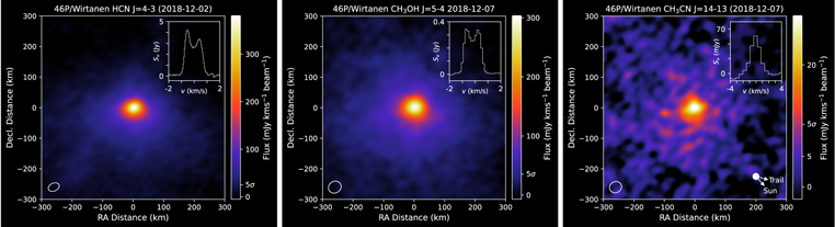
Figure 1. Spectrally integrated ALMA emission maps of HCN, CH3OH, and CH3CN, centered on their respective emission peaks. Beam size (FWHM of a Gaussian fit to the PSF) is shown in the lower-left corner. Insets show the molecular spectra on a cometocentric velocity scale, integrated within a 5″ diameter aperture centered on the brightness peak. The (sky-projected) direction of the comet’s orbital trail and comet–Sun vector are shown for CH3CN in the lower-right corner. Five times the rms noise level (5σ) is indicated on the color bar for each species ( , σ(CH3OH) = 7.1, and
  mJy km s−1).
Download figure:
Standard image High-resolution image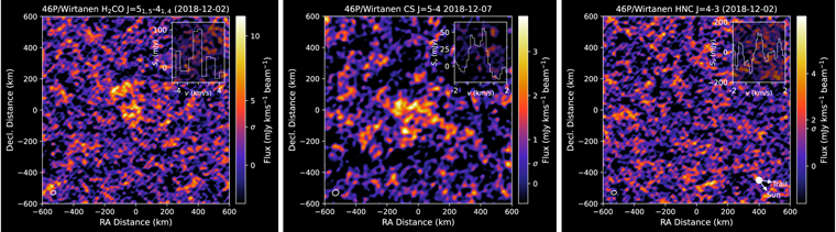
Figure 2. Same as Figure 1 but for H2CO, CS, and HNC. The H2CO and HNC maps are centered on the position of the HCN emission peak relative to the phase center, while the CS map is centered on the CH3OH peak. In the inset spectrum, the H2CO data have been binned over eight spectral channels for display. The rms noise level (σ) is indicated on the color bar for each species (σ(H2CO) = 3.0, σ(CS) = 0.5, and σ(HNC) = 1.6 mJy km s−1).
Download figure:
Standard image High-resolution imageThe insets in the upper-right corners of Figures 1 and 2 show the spectral line fluxes of each species as a function of cometocentric Doppler velocity integrated within a 5″ diameter circle centered on the comet. For CH3OH, the inset spectrum represents an average of the five strongest spectroscopically distinct (unblended) lines, whereas for CH3CN, the four strongest lines were averaged. The autocorrelation spectra for each species are shown in Figure 3. For HNC, emission is clearly detected in the autocorrelation spectrum but not in the interferometric data.
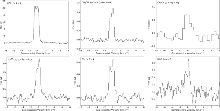
Figure 3. ALMA autocorrelation (total power) spectra in the rest frame of the comet. The spectra have been baseline-subtracted and corrected for the nominal ALMA beam efficiency (see text). The CH3OH spectrum is the mean of the five strongest unblended lines.
Download figure:
Standard image High-resolution imageIn contrast to the interferometric data, which have a spatial resolution of ∼03–0
6 (see Table 1), or 26–38 km at the distance of the comet, and are insensitive to any structures on the sky larger than ∼3″–6″ (260–410 km), the autocorrelation spectra contain flux from the entirety of the ALMA primary beam (which has an FWHM = 16″–24″). Due to the extended nature of the cometary coma (spanning hundreds of arcseconds), the autocorrelation spectra contain intrinsically more flux per beam, especially for gases that have increasing abundances as a function of distance from the nucleus. The weaker, more spatially extended appearance of the H2CO, CS, and HNC emission maps, combined with the relative strength of their autocorrelation spectra, is therefore characteristic of a more extended spatial distribution for these species, consistent with their release in the coma as daughter/distributed species. On the other hand, the strongly centrally peaked morphologies for HCN, CH3OH, and CH3CN are indicative of their production as parent species directly from the nucleus. However, considering that the observed flux distributions result from a complex interplay between molecular excitation and emission processes in a 3D outflowing coma, detailed radiative transfer modeling is required to reliably determine the molecular origins and derive production scale lengths.
4. SUBLIME Radiative Transfer Modeling
4.1. Model Physics and Geometry
Our modeling approach follows a similar method to the previous comet interferometry studies by Boissier et al. (2007), Cordiner et al. (2014), and Roth et al. (2021a). Here the interferometric visibilities are modeled using a non-LTE radiative transfer code called SUBlimating gases in LIME (SUBLIME), where LIME is the LIne Modeling Engine (Brinch & Hogerheijde 2010) from which our code is adapted. The SUBLIME model used in the present study is time dependent (in contrast to the steady-state LIME code), and takes into account the detailed molecular excitation and emission processes that occur in the presence of varying coma density, temperature, and abundance distributions (see Cordiner et al. 2022 for details). The model incorporates a Haser (1957) radial density profile and treats coma molecules as parent species, photochemical daughter species, or a mixture of both expanding outward at a constant velocity. However, our method differs from the 1D modeling performed by earlier interferometric studies, as we adopt a two-component description of the outflowing gases in three dimensions, similar to that used for the analysis of single-dish CO spectral/spatial observations of comet C/2016 R2 (PanSTARRS) by Cordiner et al. (2022).
The coma is divided into two solid-angle regions (Ω1, Ω2), each with an independent water production rate (Q1, Q2), outflow velocity (v1, v2), and kinetic temperature as a function of radius (T1(r), T2(r)). As shown in Appendix A (Figure 8), the first solid-angle region (Ω1) is defined by a cone of half-opening angle θjet with its apex at the center of the nucleus and its axial vector pointing at a phase angle ϕ with respect to the observer and at a position angle ψ in the plane of the sky. The second region (Ω2) represents the remaining (ambient) coma. This geometry, although still likely to be highly simplified compared to reality, represents an evolution from the two-hemisphere coma model of Roth et al. (2021b), which was successfully used for the analysis of asymmetric CH3OH spectra observed in 46P using the ALMA 7 m array (Atacama Compact Array, ACA). As explained by Cordiner et al. (2022), the SUBLIME model provides a sufficiently good approximation to the structure of a coma with a single dominant, rapidly expanding (near-)sunward-facing jet embedded in a slower-moving ambient coma. The adopted geometry is found to reproduce very well the spectral line profiles (including asymmetries) observed for all of our detected species while keeping the number of variable model parameters at a minimum.
The radial distribution of a daughter species is governed by its parent scale length (Lp ), which, in a uniformly expanding coma of outflow velocity v, is related to the photodissociation rate (Γ) of its parent species by Lp = v/Γ. For consistency, we assume that Γ is constant for a given parent species across both coma solid-angle regions (Ω1, Ω2), so the ratio of production scale lengths for a daughter species in those two regions is determined by the ratio of outflow velocities (v1/v2). Consequently, rather than reporting parent scale lengths for both regions, we report only the Lp value corresponding to the jet component (Ω1). Outflow velocities for daughter species in our model are allowed to differ from the parents. Daughter production rates in the two coma solid-angle regions are also independently optimized; reported daughter abundances are therefore taken as averages over the entire coma.
The excitation calculation in our model takes into account radiative cooling of rotational levels, (de-)excitation by collisions with H2O and electrons, and pumping by the solar radiation field as the gas moves outward (see Cordiner et al. 2022). The impact of coma opacity on the molecular excitation is negligible for the observed species in this comet, so radiation trapping effects are not included. We adopt H2O–HCN collision rates from Dubernet & Quintas-Sánchez (2019; also assumed to apply to HNC), while collision rates of H2O with CH3OH, H2CO, CH3CN, and CS are assumed to be the same as for H2 and have been taken from the LAMDA database (van der Tak et al. 2020). An electron density scaling factor of xne = 0.2 is used, following the recommendations of Hartogh et al. (2010) and Biver et al. (2019, 2021). Pumping rates for HCN, HNC, H2CO, and CS were calculated as described by Cordiner et al. (2019) and Roth et al. (2021b) based on the method of Crovisier & Encrenaz (1983), with rovibrational transition data from the latest versions of the HITRAN and GEISA catalogs (Delahaye et al. 2021; Gordon et al. 2022). The CH3OH pumping rates were calculated similarly. However, the Einstein A coefficients for CH3OH in the HITRAN catalog were found to be incorrect because they were calculated by considering corrupted statistical weights and partition functions. On the other hand, the HITRAN line intensities at 296 K are accurate, so by converting these to A coefficients and employing accurate statistical weights and partition functions (Villanueva et al. 2012), the required spectroscopic information could be recovered. We further complemented the HITRAN data by adding rovibrational transitions from the strong v2, v3, and v9 bands from the quantum band models of Villanueva et al. (2012). The data were then homogenized based on the CH3OH quantum numbers and energies reported for the ground-state Hamiltonian by Mekhtiev et al. (1999).
4.2. Model Optimization Strategy
Our ALMA observations were obtained on two dates: 2018 December 2 and December 7 (see Table 1). On December 2, the coma physical structure (characterized by the ratio of production rates in the sunward jet versus ambient coma, Q1/Q2, and the jet properties, θjet, ϕ, and ψ) was determined using a model fit to the bright HCN J = 4–3 line observations. On December 7, multiple lines from the CH3OH (JK = 5K –4K ) band were used instead, since HCN was not observed on this date. Both of these species correlate well with H2O (Dello Russo et al. 2016a; Bockelée-Morvan & Biver 2017) and therefore provide a reasonable proxy for the overall coma outflow velocity and Q1/Q2 ratio in the absence of spectrally resolved H2O data. The H2O coma physical structure derived from fitting the HCN data was therefore used in our models for H2CO and HNC (also obtained on December 2), whereas the structure derived using CH3OH was applied to CH3CN and CS. For CH3CN, the observed ALMA data were of insufficient spectral resolution to adequately constrain the values of v1 and v2, whereas for H2CO, HNC, and CS, the correlation with H2O is insufficiently demonstrated, and the data were of insufficient signal-to-noise ratio (S/N) to reliably constrain the coma structure by themselves.
The total H2O production rate on each date was obtained from a linear fit to the measurements between December 2 and December 10 by Combi et al. (2020) using Lyα observations by the Solar and Heliospheric Observatory satellite, which gave Q(H2O) = 6.1 × 1027 s−1 on December 2 and Q(H2O) = 7.2 × 1027 s−1 on December 7. These values are consistent with a slow increase in Q(H2O) as the comet approached perihelion on December 12 and are in line with the average values of 8 × 1027 s−1 measured by Lis et al. (2019) using the Stratospheric Observatory for Infrared Astronomy between December 14 and December 20 and 7 × 1027 s−1 measured using the Infrared Telescope Facility (IRTF) between December 6 and December 21 (Khan et al. 2023).
Our models were set up on a 3D Delaunay grid containing 10,000 points distributed pseudorandomly with a density of points proportional to the logarithm of the radial distance (r) from the center of the nucleus (excluding the nucleus itself). The model domain therefore consisted of a spherical coma region extending from the surface of the nucleus (assumed to be a sphere of radius 500 m) to an outer boundary at r = 2 × 10⁵ km. The outer boundary was chosen to be large enough so that further increasing it had no significant impact on our model results. Ray tracing was performed along the line-of-sight vectors through each grid point on a frequency grid with a uniform channel spacing of 100 m s−1, which was then interpolated in two (spatial) dimensions onto the image grid, which consisted of 768 × 768 pixels of 01 in size. The innermost 4 × 4 pixel region of the image was further supersampled using a 30 × 30 point Cartesian grid to accurately capture the nonlinear behavior of the coma flux on the smallest relevant radial scales. To simulate the response of the ALMA primary beam, each plane of the synthetic image cubes was multiplied by a 2D Gaussian of FWHM = 1.13λ/D, where λ is the wavelength, and D is the antenna diameter. For each molecule, the frequency axis of the resulting synthetic image cube was convolved to the spectral resolution of the ALMA observations, followed by cubic spline interpolation to the observed frequency grid. This allowed a channel-by-channel comparison of the model with the observations.
Interferometric observations inherently suffer from incomplete spatial sampling, and the resulting Fourier-transformed images can be subject to artifacts introduced by gridding, interpolation, and numerical deconvolution. To facilitate accurate modeling of the data and avoid our model fits becoming biased by image artifacts, we chose to perform all model fitting in the Fourier domain. This requires taking the Fourier transform of the simulated coma image cubes, then sampling each spectral channel with the same set of uv points (antenna baseline lengths and orientations) as the observations, which was performed using the vis_sample code (Loomis et al. 2018). To make the problem computationally tractable, the observed visibilities were first averaged along the time axis to produce a single (complex) visibility point per baseline per channel. The χ2 statistic,
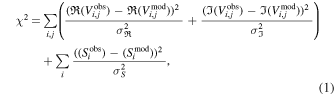
was minimized using lmfit (Newville et al. 2016) by application of the Levenberg–Marquardt algorithm. Summation of the interferometric residuals (the difference between Vobs for the observations and Vmod for the model) was performed over the set of baselines j = N(N − 1), where N is the number of ALMA antennas (43), and i is the number of spectral channels. Due to the presence of coma asymmetries, both the real  and imaginary
  parts of the complex visibilities were included in the χ2 calculation. The differences between the model total power spectra (Smod
i
) and the observed autocorrelation spectra (Sobs
i
) provide additional strong constraints on the production scale length (Lp
) of each species due to the larger angular scales probed by these data. During fitting, the residuals were scaled by the respective standard deviations of the real and imaginary visibilities and the autocorrelation spectra (
parts of the complex visibilities were included in the χ2 calculation. The differences between the model total power spectra (Smod
i
) and the observed autocorrelation spectra (Sobs
i
) provide additional strong constraints on the production scale length (Lp
) of each species due to the larger angular scales probed by these data. During fitting, the residuals were scaled by the respective standard deviations of the real and imaginary visibilities and the autocorrelation spectra ( ,
,  , and σS
), which were calculated from line-free data regions adjacent to each spectral line.
, and σS
), which were calculated from line-free data regions adjacent to each spectral line.
To allow for errors in the comet ephemeris coordinates, a positional (R.A., decl.) offset of the model origin from the image center was included as a further pair of free parameters in the model fits. Statistical uncertainties on all model parameters were obtained from the diagonal elements of the lmfit covariance matrix.
4.3. Coma Temperature Structure Derived from CH3OH Visibilities
Model optimization was performed first for CH3OH because the multiple transitions observed for this species span a broad range of upper-state energy levels (see Table 2), which allows its rotational excitation state, from which the coma kinetic temperature is derived, to be determined (see, e.g., Cordiner et al. 2017a; Biver et al. 2021). Our method differs from previous studies, however, due to our model’s ability to interpret the coma temperature structure in three dimensions by fitting the variations in individual CH3OH spectral line channels (Vi , Si ) as a function of spatial (uv) coordinate.
We began with the simplest assumption of a constant kinetic temperature (T) as a function of radius, then added complexity to the T(r) profile until a good fit to the data was obtained. This strategy keeps the number of free parameters at a minimum (therefore keeping the χ2 minimization computationally feasible) and ensures that there are enough degrees of freedom in the model to reproduce the data but not so many that the model becomes ill-constrained. To obtain a good fit to the observations, it was necessary to implement different temperature profiles as a function of radius (T1(r), T2(r)) within the two different coma solid-angle regions. Temperature variability was implemented using a segmented linear function (in  –T space, within the domain
  to θPB), with a variable number of segments (n) of equal length (ls
) in
to θPB), with a variable number of segments (n) of equal length (ls
) in  space. The segmented function was smoothed (in
  space) by convolving it with a Gaussian of FWHM equal to ls
. The temperature was set constant inside a radius corresponding to half the minor axis of the ALMA beam (
space) by convolving it with a Gaussian of FWHM equal to ls
. The temperature was set constant inside a radius corresponding to half the minor axis of the ALMA beam ( ) and outside a radius corresponding to half the primary beam FWHM (r = θPB/2). A good fit to the entire CH3OH data set was obtained using n = 5 variable points in the temperature profiles as a function of radius (see Figure 4 and Appendix B, Figure 9).
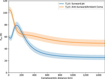
Figure 4. Variation of the 46P coma kinetic temperature with radius in the sunward (jet) and antisunward (ambient) coma regions, derived from modeling the CH3OH J = 5–4 data. Shaded regions indicate the ±1σ error envelopes.(The data used to create this figure are available.)
Download figure:
Standard image High-resolution imageDue to the high S/N of our CH3OH observations, the best-fitting coma model is tightly constrained by the data and has a jet half-opening angle of θjet = 70° ± 5° with a phase angle of ϕ = 38° ± 1° and position angle of ψ = 33° ± 1°. The resulting model jet emanates from close to (within 10° of) the subsolar point on our (assumed) spherical nucleus and is therefore consistent with preferential outgassing in the general sunward direction. The best-fitting jet outflow velocity is v1 = 0.729 ± 0.002 km s−1, with the remaining (ambient/nightside) coma expanding at v2 = 0.395 ± 0.003 km s−1. We initially attempted to fit the observed ALMA data assuming that CH3OH was solely a parent species, but a significant (15σ) improvement in the final χ2 value was obtained using a composite (parent + daughter) model. Independent optimization of the parent and daughter CH3OH production rates resulted in approximately equal abundances for both components of 1.2% ± 0.1% (relative to H2O), with a best-fitting parent scale length of Lp = 36 ± 7 km for the CH3OH daughter (in the jet component, Ω1). The presence of an additional CH3OH daughter component implies the production of significant amounts of CH3OH in the near-nucleus coma, likely from the sublimation of icy grains (see Section 5.2). We also attempted to fit the CH3OH data using a pure daughter model, but this resulted in a statistically worse fit at the 11σ level, so our modeling strongly implies the presence of both nucleus (parent) and coma (daughter) sources for CH3OH in comet 46P (see also Section 4.4).
A comparison between the best-fitting modeled and observed visibility spectra is shown in Appendix B (Figure 9), which includes the total power (autocorrelation) spectrum at the top, followed below by the real part of the interferometric visibilities, binned within successive 20 m baseline ranges. The angular scales probed decrease with increasing baseline length, from the 24″ scale of the autocorrelation spectrum down to the 06 scale probed by the longest baselines. We show only the real part of the visibilities, since the imaginary components are weak and noisy.
As shown in Figure 4, the average temperature on the sunward (jet) side of the nucleus is significantly lower than the antisunward (ambient) side. This is particularly true closest to the nucleus (within r = 19 km), where T1 = 59 ± 3 and T2 = 105 ± 5 K, amounting to almost a factor of 2 difference. The temperature in the sunward jet rises with increasing cometocentric distance, reaching a peak with T1 = 79 ± 5 K at r = 121 km (compared with T2 = 71 ± 5 K in the ambient coma at the same radius) before falling smoothly toward T1 = 25 ± 4 K (T2 = 49 ± 6 K) at large radii (r > 1500 km). The different temperature behavior on opposite sides of the nucleus is remarkable, since it implies significant differences in the balance of heating and cooling mechanisms on the sunward and antisunward sides of the comet. Biver et al. (2021) also identified cooler gas on the dayside of the nucleus than the nightside (57 versus 71 K) based on single-dish CH3OH observations probing coma radial distances of ≲600 km. This is qualitatively similar to our result and was explained by Biver et al. (2021) as being due to more efficient adiabatic cooling on the sunward side (for further discussion, see Section 5.2).
The observed transitions of CH3CN from different K levels provide an additional measure of the coma temperature. However, due to the lower spectral resolution and S/N, it was not possible to reliably constrain the spatial distribution of temperatures for this species. Assuming a constant temperature throughout the coma, we found T = 80 ± 8 K using the CH3CN data.
4.4. Visibility Modeling to Derive Parent Scale Lengths
Adopting the best-fitting coma kinetic temperature distribution from our CH3OH modeling, we proceeded to optimize the remaining free model parameters for HCN, HNC, CS, H2CO, and CH3CN. As a result of a lower S/N and spectral resolution for CS and CH3CN (simultaneously observed with CH3OH), we employed the same jet opening angle (70°) and ratio of H2O production rates as derived for CH3OH (Q1/Q2 = 1.21). The HCN jet opening angle (70°) and Q1/Q2 ratio (1.33) were employed for modeling the HNC and H2CO data (observed on the same date). The best-fitting HCN coma outflow velocities were v1 = 0.741 ± 0.001 and v2 = 0.443 ± 0.001 km s−1, with a jet phase angle ϕ = 44° ± 1° and position angle ψ = 37° ± 1°, consistent with preferential outgassing in the sunward direction. The jet axis was therefore fixed along the comet–Sun vector for all species apart from CH3OH (see Section 4.3). Model fits to the binned visibility spectra for all molecules are shown in Appendix B (Figures 9– 14). Since the visibility data for CH3CN, H2CO, CS, and HNC are noisier than for CH3OH and HCN (particularly on large baselines), some of the longer baseline ranges for which no signal is evident have been omitted from Figures 11–14.
To visualize the radial flux distribution for each molecule, in Figures 5 and 6, we plot the real part of the interferometric visibility as a function of baseline length (uv distance). The observed and modeled fluxes are averaged across the spectral channels containing line emission, and the interferometric data have been further averaged into 10 m wide uv bins. Statistical error bars on the interferometric data are typically very small due to the large number of data points being averaged together, whereas the total power data points have an additional 10% error added in quadrature with the statistical error to allow for uncertainty in the aperture efficiency of the ALMA antennas. For HCN, a parent outgassing model provides the best fit to the data. In an attempt to better fit the total power (uv = 0) data point, a daughter distribution of HCN was added, and the model parameters were reoptimized (with variable parent and daughter abundances and HCN parent scale length Lp ). However, this did not significantly improve the χ2 value, and the optimized Lp value was found to be 5 ± 16 km, which is consistent with zero, showing that HCN is likely a parent species.
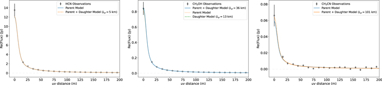
Figure 5. Observed interferometric visibilities for HCN, CH3OH, and CH3CN, with the best-fitting models overlaid. The observations and model data have been (spatially) averaged within 10 m uv bins and (spectrally) averaged over all line emission channels for each species, including 13 lines for CH3OH and five lines for CH3CN. The zero-spacing data points (at uv = 0) were taken from the ALMA autocorrelations (observed simultaneously with the interferometric data). The preferred best-fitting visibility models are shown with solid lines, while dashed and dotted curves show models that are ruled out based on a poorer quality of fit (or other criteria; see text).
Download figure:
Standard image High-resolution imageThe binned CH3OH visibilities and corresponding model fits are shown in Figure 5 (middle panel). As explained in Section 4.3, in contrast to HCN, a parent + daughter model provides the best fit for CH3OH (with Lp
= 36 ± 7 km for the daughter component). The difference between the CH3OH parent and parent + daughter models is difficult to see in Figure 5; unbinned, zoomed CH3OH visibilities are therefore shown in Appendix B (Figure 15), where the improved fit for the parent + daughter model is evident. For CH3CN, a parent model fits the data very well. Addition of a CH3CN daughter component slightly improved the fit (resulting in  km for the daughter), but the associated drop in χ2 value corresponded to only 1.6σ, so the improvement in fit quality was not statistically significant.
The binned visibility data for H2CO, CS, and HNC are plotted in Figure 6, and as shown by the overlaid model curves, these three species can only be well fit using daughter models (their respective best-fitting parent scale lengths are given in Table 3). To obtain the best visibility fits for these daughter species, we allowed their outflow velocities to differ from those of the underlying H2O distribution (determined from our HCN and CH3OH models), which may be physically justified if they originate from a nonnucleus source. We also attempted to fit these data using “parent-only” models by setting Lp = 0 and optimizing the abundance to obtain the best fit to the observations. However, in all three cases, a parent model provides a clearly inadequate fit, particularly at the largest scales probed by the total power (uv = 0) data. For CS, we also tried to fit the observations assuming production of this species from CS2 photolysis (at a photodissociation rate of Γ = 2.61 × 10⁻³, which corresponds to Lp = 280 km in the jet and Lp = 152 km in the ambient coma; Huebner & Mukherjee 2015). As shown by the dashed orange curve, the CS2 photolysis model produces insufficient CS flux on large scales (small uv values) to reproduce the observations. The final best-fitting model parameters for all species are given in Table 3.
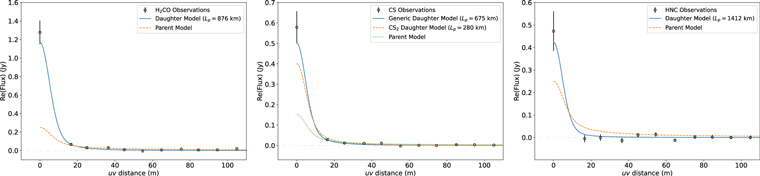
Figure 6. Same as Figure 6 but for H2CO, CS, and HNC.
Download figure:
Standard image High-resolution imageTable 3. 3D Visibility Modeling Results
| Species | Abundance a (%) | v1 (km s−1) | v2 (km s−1) | Lp (km) |
|---|---|---|---|---|
| HCN |

| 0.741 ± 0.001 | 0.443 ± 0.001 | <3 |
| CH3OH b |

| 0.729 ± 0.002 | 0.395 ± 0.002 | 0/36 ± 7 |
| CH3CN |

| 0.729 c | 0.395 c | <18 |
| H2CO |

| 0.65 ± 0.02 | 0.47 ± 0.02 |

|
| CS |

| 0.66 ± 0.02 | 0.37 ± 0.02 |

|
| HNC |

| 0.69 ± 0.05 | 0.34 ± 0.05 |

|
Notes.
a Total production rate relative to H2O. b The best-fitting CH3OH model has both nucleus (parent) and coma (daughter) production; the reported abundance is a sum over both components. c Held fixed at the CH3OH values (simultaneously observed) due to the low spectral resolution for CH3CN.Download table as: ASCIITypeset image
Due to the inverse exponential behavior of cometary molecular densities as a function of radius, uncertainties on the parent scale lengths can be highly asymmetric and are therefore not adequately represented using the symmetric error bars obtained from the lmfit covariance matrix. To address this issue, we calculated the χ2 surface for each species as a function of Lp
(with the abundance as a variable but other model parameters held fixed) and plotted the resulting Δχ2(Lp
) curve with cubic spline interpolation between the points (with  , where
  is the minimum value). The results are shown in Figure 7, with dotted horizontal lines showing the 1σ (68% confidence) Δχ2 thresholds and dashed horizontal lines showing the 2.6σ (99% confidence) thresholds.
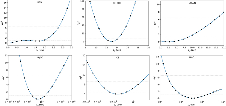
Figure 7. Parent scale length χ2 analysis for our observed species in 46P, showing the change in χ2 value (Δχ2) as a function of parent scale length (Lp ). Dotted horizontal lines show the Δχ2 = 1 threshold (1σ), corresponding to 68% confidence, and dashed horizontal lines show the Δχ2 = 6.63 threshold (2.6σ), corresponding to 99% confidence.
Download figure:
Standard image High-resolution imageFor HCN, the χ2 minimum is for Lp = 0, confirming that this species is a parent. For CH3CN, the smallest χ2 value occurs around Lp = 2.5 km, but this minimum is much shallower than 1σ and therefore not significant. The CH3CN Δχ2 curve crosses the 99% confidence threshold at Lp = 18 km, which represents a strict upper limit on the scale of possible coma production for this species assuming a single (distributed) source. On the other hand, CH3OH shows a well-defined χ2 minimum at Lp = 13 km. However, as explained in Section 4.3, a composite (parent + daughter) model provides the best fit for this species (with a lower χ2 value than the pure daughter model plotted here); the Lp value of the daughter component in the CH3OH composite model is well constrained as 36 ± 7 km, so this is reported in Table 3 instead.
Assuming a scale length of Lp = 36 km for a sublimating icy grain source (i.e., the same as derived for CH3OH), the abundance upper limit (at the 99% confidence level) for icy grain production of HCN is <0.001% relative to H2O. This corresponds to <1% of the total HCN. The associated upper limit for icy grain production of CH3CN is <0.01%, which is comparable to the measured CH3CN parent abundance and shows that a significant source of CH3CN production from icy grains in the coma, close to the nucleus, cannot be ruled out by our data.
The H2CO, CS, and HNC all exhibit well-defined χ2 minima at substantially larger Lp
values than the other observed species, so these molecules are confirmed as originating primarily in the coma of comet 46P, rather than from the nucleus. While the H2CO and CS Lp
values are well constrained (at  and
and  km, respectively), the HNC uncertainty interval is much larger and highly asymmetric, with an Lp
value lying between 1045 and 14,880 km (at 1σ confidence). At the stricter, 99% confidence level, the Lp
(HNC) value is only constrained by a lower limit of >218 km.
km, respectively), the HNC uncertainty interval is much larger and highly asymmetric, with an Lp
value lying between 1045 and 14,880 km (at 1σ confidence). At the stricter, 99% confidence level, the Lp
(HNC) value is only constrained by a lower limit of >218 km.
5. Discussion
5.1. HCN
The high spatial resolution of ALMA combined with the close geocentric distance of 46P places unusually tight constraints on the production scale length of HCN. With an upper limit of Lp < 3 km, it is likely that HCN originates primarily from outgassing by the nucleus of the comet. At an outflow velocity of 0.74 km s−1 (in the sunward jet), any HCN daughter production would need to occur on a timescale of <4 s, which is significantly shorter than the lifetimes of any known coma molecules (typically in the range of 103–106 s; Huebner & Mukherjee 2015). Our scale length upper limit is consistent with (although significantly better constrained than) the previous upper limits of Lp < 50 km in C/2012 F6 (Lemmon) and C/2012 S1 (ISON) (Cordiner et al. 2014) and Lp < 100 km in C/2015 ER61 (Roth et al. 2021a), which were obtained using ALMA and ACA data. Including the IRAM Plateau de Bure interferometric study of comet Hale–Bopp (Wink et al. 1997) and the Keck NIRSPEC study of C/2014 Q2 (Lovejoy), the body of evidence demonstrating HCN release from direct sublimation of nucleus ices with no clear evidence for production in the coma is now substantial. Coma HCN abundance measurements in fully activated comets thus provide a valid proxy for the abundance of this molecule in the nucleus ices.
Our derived HCN abundance is 0.1176% ± 0.0003% with respect to H2O, with the error bar only accounting for statistical uncertainties. Adopting a conservative estimate for the ALMA flux scale uncertainty of 10% and an extra uncertainty of 10% in the H2O production rate (added in quadrature), the abundance error increases to ±0.016%. Our measured HCN abundance in comet 46P is therefore consistent with the value of 0.11% ± 0.01% obtained by Biver et al. (2021) within the same month and matches the average value observed previously in OCCs and JFCs using radio spectroscopy (Bockelée-Morvan & Biver 2017).
5.2. CH3OH
Our observations reveal the presence of two coexisting outgassing modes for CH3OH, consisting of production (1) directly from the nucleus and (2) from a near-nucleus coma source with Lp = 36 ± 7 km. Our best-fitting SUBLIME model indicates that both sources are responsible for similar amounts of CH3OH production, with best-fitting abundances (with respect to H2O) of 1.19% ± 0.13% for the nucleus (parent) source of CH3OH gas and 1.18% ± 0.13% for the distributed (coma) source.
The presence of icy grain sublimation has been known to be an important source of gases in cometary comae since the EPOXI mission to comet 103P/Hartley 2 (A’Hearn et al. 2011). Using infrared spectroscopy, Protopapa et al. (2014) observed 1 μm sized water-ice grains in the coma of 103P, while Kelley et al. (2013) observed a halo of larger, longer-lived ice chunks (with sizes ≥1 cm) surrounding the nucleus at distances of up to ∼40 km. Using a detailed DSMC coma model, Fougere et al. (2013) determined that 77% of the H2O outgassing in 103P originates from sublimation of icy grains in the coma. Such an excess of H2O production compared with its small nucleus size led to 103P being designated as a “hyperactive” comet.
Comet 46P/Wirtanen is also hyperactive (Lis et al. 2019; Moulane et al. 2023), and the large H2O production rate for its nucleus size can, at least in part, be attributed to the presence of icy grains in the coma (Bonev et al. 2021). Knight et al. (2021) explained the different OH and CN morphologies in 46P as being partly due to OH production from an icy grain H2O source. However, Protopapa et al. (2021) excluded pure H2O-ice grains in the coma of this comet. Based on the nondetection of H2O-ice absorption features, these authors suggested two possible explanations for the hyperactivity of 46P: icy grains (∼1 μm in size) containing a small amount of low-albedo dust or larger chunks ejected from the nucleus containing significant amounts of water ice. Previous ALMA observations by Cordiner et al. (2017a) identified nucleus outgassing as the primary source of CH3OH in the coma of C/2012 K1 (PanSTARRS). On the other hand, a distributed CH3OH source (with a scale length of ∼550 km) was observed using the James Clerk Maxwell Telescope (JCMT) in comet 252P/LINEAR and attributed to CH3OH production from icy grains in the coma (Coulson et al. 2017). It is therefore reasonable to attribute the source of our observed CH3OH daughter distribution in 46P (around 40 km from the nucleus) to the presence of sublimating icy grains in the coma composed of a mixture of CH3OH, H2O, and dust. The sublimation rate of coma icy grains depends on their size and composition. Based on the calculations of Beer et al. (2006) and assuming that the gas and dust outflow velocities are coupled, our derived lifetime of 496 ± 97 s for the CH3OH-producing grains in 46P implies a dirty ice grain size of ∼10 μm. If the dust is moving outward more slowly than the gas, then the grains could be larger.
The presence of sublimating icy grains can significantly impact the coma temperature, as shown by the direct-simulation Monte Carlo (DSMC) models of Fougere et al. (2012) and Fougere (2014), due to the transfer of excess kinetic energy from sublimated molecules to the surrounding gas. In the absence of such a mechanism, the gas kinetic temperature in coma physical models (e.g., Rodgers et al. 2004; Tenishev et al. 2008) falls rapidly with distance from the nucleus, from ≳100 K at r = 0 to ∼10 K at r = 100 km, due to quasi-adiabatic expansion. Such steeply declining temperatures are at odds with coma observations. For example, the observations of comets 73P/Schwassmann–Wachmann B, 103P/Hartley 2, C/2012 S1 and 46P/Wirtanen (Bonev et al. 2008, 2013, 2014, 2021), and C/2012 K1 (Cordiner et al. 2017a) revealed a shallower temperature decay—and, in some cases, increasing temperatures—as a function of radius, attributable to sublimative heating. Spatially resolved temperature observations therefore provide an indirect probe for the presence of icy grains in cometary comae.
Our derived 46P coma kinetic temperature profile (Figure 4) shows an initial increase with radius on the sunward side of the nucleus, followed by a relatively slow decrease, consistent with strong coma heating due to the sublimation of icy grains within a few hundred kilometers of the nucleus. On the antisunward side, the temperature drop is also less steep than predicted by hydrodynamical and DSMC models for other comets and flattens out to a higher temperature than predicted without the presence of icy grain heating (Rodgers et al. 2004; Tenishev et al. 2008; Fougere et al. 2012). This temperature behavior therefore suggests the presence of significant icy grain sublimation in the 46P coma, consistent with conclusions based on spatially resolved infrared observations of H2O in this comet (Bonev et al. 2021). Dedicated theoretical modeling will be required to further investigate this hypothesis.
Our total CH3OH abundance of 2.7% ± 0.1% including the nucleus and coma sources is consistent (at the 2σ level) with the value of 3.03% ± 0.23% observed by Bonev et al. (2021) on 2018 December 18 but somewhat smaller than the value of 3.38% ± 0.03% observed by Biver et al. (2021) during December 11–18 and larger than the value of 1.6% ± 0.1% observed by Bergman et al. (2022) during December 22–28. These differences could be explained by temporal variability of the CH3OH and H2O outgassing rates, since significant short-timescale variations in Q(CH3OH) (over a period of several hours to several days) were observed in this comet by Roth et al. (2021b). Indeed, our CH3OH production rate of (1.9 ± 0.1) × 1026 s−1 on December 7 is very close to the value of (2.2 ± 0.1) × 1026 s−1 observed on December 6 by Khan et al. (2023) and (2.1 ± 0.1) × 1026 s−1 on December 11 (Biver et al. 2021), demonstrating good consistency between the ALMA, IRTF, and IRAM measurements in this case.
The presence of an icy grain source for CH3OH but not HCN implies that the icy grains are chemically distinct from the bulk (sublimating) ice within the nucleus. Drahus et al. (2012) also inferred the presence of icy grain sources of CH3OH and HCN in comet 103P and concluded that CH3OH is more intimately mixed with H2O ice than HCN, with a larger abundance of CH3OH in the icy grains. The apparent dichotomy between the abundances of CH3OH and HCN in the two cometary ice storage reservoirs (icy grains versus bulk nucleus) was interpreted by Drahus et al. (2012) as due to thermal evolution of the nucleus. A primordial origin in the protoplanetary disk or interstellar cloud prior to accretion of the comet is also possible. Spatial differentiation of O- and CN-rich molecules between the gas and ice phases has been observed in disks (Bergner et al. 2018; Booth et al. 2021; Öberg & Bergin 2021), indicating that an active carbon chemistry occurs in the gas phase, while O-bearing species such as CH3OH and H2O remain largely frozen on grains. Nonuniform mixing of these distinct chemical reservoirs during comet accretion could lead to the observed spatial heterogeneity of the CH3OH/HCN ratio within the nucleus.
5.3. CH3CN
A production scale length upper limit of Lp < 18 km was derived for CH3CN based on our visibility modeling. The ALMA data show no significant evidence for production of this molecule as a coma daughter species (either from photolysis of a parent molecule or from sublimation of icy grains), so we conclude that the primary source of CH3CN is from direct sublimation of molecular ices in the nucleus. The abundance of this molecule (0.011% ± 0.002%) is consistent with but toward the lower end of the range of values (0.008%–0.054%) previously observed in comets (Bockelée-Morvan & Biver 2017).
This is the most complex nitrile confirmed to be present in cometary ice to date. It has long been detected in the gas phase in the interstellar medium and protostellar envelopes (Herbst & van Dishoeck 2009), while recent studies using ALMA have found CH3CN to be widespread in protoplanetary disks, where it is believed to be formed primarily via chemistry on grain surfaces (Öberg et al. 2015; Bergner et al. 2018; Ilee et al. 2021) before being thermally desorbed into the gas phase, where it can be observed. So far, CH3CN has not been detected in interstellar ices, but our measured abundance in 46P is consistent with the upper limit of ≲2% (with respect to H2O) found recently along two interstellar sight lines using the James Webb Space Telescope (McClure et al. 2023).
The CH3CN/HCN ratios we measure in 46P are consistent with or somewhat higher than the values observed in nearby protoplanetary disks by Bergner et al. (2018) and Ilee et al. (2021), implying a likely genetic relationship between the protoplanetary disk and cometary nitriles. Our observed CH3CN/H2O ratio also matches that found in the (gas plus ice) phase of the GM Aur planet-forming disk by Ilee et al. (2021) but is ∼eight times lower than that found in the AS 209 disk. The utility of such comparisons is limited, however, due to the action of gas-phase chemical processes, which can modify the CH3CN/HCN/H2O ratios found in the disk gas compared with those in the ice. Cometary observations therefore remain a perhaps more useful probe of the abundances of complex nitriles in the ice reservoir of our solar system’s planet-forming disk.
5.4. H2CO
Our measured H2CO production scale length of  km at rH = 1.07 is compatible with the values measured previously using ALMA of
  km at rH = 1.17 au in C/2015 ER61 (PanSTARRS) (Roth et al. 2021b),
  at rH = 1.47 au in C/2012 F6 (Lemmon), and 280 ± 50 at rH = 0.54 au in C/2012 S1 (ISON) (Cordiner et al. 2014). When scaled by
  , these Lp
values are in reasonably close agreement, consistent with H2CO production by photodissociation of a (molecular) parent species at a rate of ∼7 × 10⁻⁴ s−1 (at rH = 1 au) in an optically thin coma. However, Biver et al. (1999) measured a much larger Lp
value of
, these Lp
values are in reasonably close agreement, consistent with H2CO production by photodissociation of a (molecular) parent species at a rate of ∼7 × 10⁻⁴ s−1 (at rH = 1 au) in an optically thin coma. However, Biver et al. (1999) measured a much larger Lp
value of  km in comet C/1996 B2 (Hyakutake) using a single-dish radio telescope, and Meier et al. (1993) derived Lp
∼ 3600 km in 1P/Halley at rH = 0.89 au via in situ mass spectrometry. Photolysis of CH3OH is expected to produce H2CO in the outer coma but cannot be responsible for the observed H2CO in these comets, since it occurs at a rate of 1.0 × 10⁻⁵ s−1 at rH = 1.06 au (Huebner & Mukherjee 2015; see also Heays et al. 2017), which is almost 2 orders of magnitude smaller than the H2CO parent photodissociation rate required to fit our ALMA observations. Indeed, the corresponding CH3OH dissociation scale in the 46P sunward jet is 73,000 km, which is much larger than the maximum angular scale of 1400 km spanned by the ALMA primary beam FWHM. Alternative H2CO parents must therefore be sought.
km in comet C/1996 B2 (Hyakutake) using a single-dish radio telescope, and Meier et al. (1993) derived Lp
∼ 3600 km in 1P/Halley at rH = 0.89 au via in situ mass spectrometry. Photolysis of CH3OH is expected to produce H2CO in the outer coma but cannot be responsible for the observed H2CO in these comets, since it occurs at a rate of 1.0 × 10⁻⁵ s−1 at rH = 1.06 au (Huebner & Mukherjee 2015; see also Heays et al. 2017), which is almost 2 orders of magnitude smaller than the H2CO parent photodissociation rate required to fit our ALMA observations. Indeed, the corresponding CH3OH dissociation scale in the 46P sunward jet is 73,000 km, which is much larger than the maximum angular scale of 1400 km spanned by the ALMA primary beam FWHM. Alternative H2CO parents must therefore be sought.
The absence of other known C-, H-, and O-bearing molecules with sufficient abundances has led to the idea that H2CO may be released in the coma from the thermal breakdown of organic-rich dust particles. Formaldehyde polymer (or polyoxymethylene, POM) was found to provide a plausible explanation for the observed H2CO parent scale length in comet 1P/Halley (Cottin et al. 2004) and the heliocentric dependence of H2CO production rates observed in O1/Hale–Bopp (Fray et al. 2006). The dissociation scale length of solid-phase POM depends strongly on the particle size and temperature (Fray et al. 2006), so the observed variations in Lp (H2CO) can be explained as a result of differing size distributions for the POM-rich dust grains in the different comets observed to date. Conversely, Milam et al. (2006) noted a lack of evidence for POM in Giotto mass spectra of comet Halley and argued that it constitutes an unlikely source of H2CO in the coma. Furthermore, mass spectrometry by the Rosetta mission found no evidence for POM in comet 67P (Hänni et al. 2022), so alternative explanations may be required to explain the distributed H2CO source. Moreover, given the limited sample size and large disparity between the observed Lp (H2CO) values, it will be important to conduct more observations of H2CO distributions in different comets over a range of coma size scales at differing heliocentric distances to better characterize the behavior of the H2CO source(s) and help constrain the properties of its still-elusive parent.
By simultaneously fitting the H2CO parent scale length and production rate ratio relative to water, we derive an H2CO abundance of  %, which is smaller than the value of x = 0.38% ± 0.02% obtained from IRAM 30 m observations by Biver et al. (2021) using Lp
(H2CO) = 5000 km. This discrepancy is not surprising considering that the retrieved H2CO production rate from single-dish observations scales with the adopted Lp
value. Using Lp
= 880 km, the IRAM data are consistent with x = 0.13% ± 0.01%. The H2CO production rate of (9.1 ± 0.9) × 1024 s−1 obtained by Coulson et al. (2020) using the JCMT assuming Lp
= 860 km also matches our derived H2CO production rate. Our H2CO abundance is the second-lowest value reported in a comet to date at radio wavelengths (Bockelée-Morvan & Biver 2017), but it should be remembered that the majority of those values were obtained using assumed (rather than directly measured) Lp
(H2CO) values. We therefore emphasize the importance of using an accurate parent scale length when deriving H2CO production rates in comets.
%, which is smaller than the value of x = 0.38% ± 0.02% obtained from IRAM 30 m observations by Biver et al. (2021) using Lp
(H2CO) = 5000 km. This discrepancy is not surprising considering that the retrieved H2CO production rate from single-dish observations scales with the adopted Lp
value. Using Lp
= 880 km, the IRAM data are consistent with x = 0.13% ± 0.01%. The H2CO production rate of (9.1 ± 0.9) × 1024 s−1 obtained by Coulson et al. (2020) using the JCMT assuming Lp
= 860 km also matches our derived H2CO production rate. Our H2CO abundance is the second-lowest value reported in a comet to date at radio wavelengths (Bockelée-Morvan & Biver 2017), but it should be remembered that the majority of those values were obtained using assumed (rather than directly measured) Lp
(H2CO) values. We therefore emphasize the importance of using an accurate parent scale length when deriving H2CO production rates in comets.
An upper limit of x < 0.064% was obtained by Bonev et al. (2021) using Keck infrared observations, but this was calculated assuming H2CO release directly from the nucleus (i.e., Lp = 0)—a common assumption among infrared spectroscopists (e.g., DiSanti et al. 2006; Dello Russo et al. 2016b) due to the difficulty of deriving Lp values from infrared spatial profiles—which inevitably underestimates the total coma H2CO abundance in the presence of distributed sources. Our ALMA observations show no evidence for H2CO production by the nucleus, with a (3σ) upper limit of 0.08% on the abundance of any parent H2CO, consistent with the Bonev et al. (2021) result. The relatively short H2CO parent lifetimes derived using ALMA imply significant daughter production of H2CO in the near-nucleus coma that could, in some situations, appear similar to a parent source. Further investigations of H2CO spatial emission profiles at the angular scales of a few arcseconds probed by infrared spectroscopy are therefore warranted.
Despite the evidence for a lack of H2CO in cometary ices inferred using ALMA observations, it remains one of the most widespread gas-phase molecules in the Galaxy. Abundances of H2CO relative to water can reach several percent in warm protostellar gas (Ceccarelli et al. 2000; Ehrenfreund & Charnley 2000), while mid-infrared spectroscopy indicates possible abundances of ∼6% in ices around low-mass protostars (Boogert et al. 2015). The lack of detectable H2CO in cometary nuclei using ALMA therefore provides evidence for chemical processing to destroy H2CO ice in (or during its passage to) the protosolar disk, which is expected to occur as part of the pathway to forming more complex organic molecules (including biologically relevant species), starting with hydrogenation of H2CO to make CH3OH ice (Chuang et al. 2016). Although formaldehyde is commonly detected in the gas phase in protoplanetary disks (e.g., Pegues et al. 2020), total H2CO/H2O masses in the range of ∼10−5–10−3 were recently measured in a sample of five disks by Guzmán et al. (2021), so relatively low H2CO abundances in cometary nuclei (≲6 × 10⁻⁴, as found by our study and Bonev et al. 2021) may not be surprising.
Of relevance to the nature of the H2CO parent, it is noteworthy that the H2CO outflow velocity of 0.65 ± 0.02 km s−1 in the sunward jet is significantly less than the HCN (parent molecule) outflow velocity of 0.74 km s−1 measured only 2 hr earlier (see Table 3). Such a rapid drop in the jet velocity over this period seems unlikely, so this result may constitute evidence that the H2CO parent is flowing radially outward at a slower rate than the gases sublimating directly from the nucleus. A similar effect is also observed for the daughter species CS (observed simultaneously with CH3OH), as well as HNC (albeit at lower confidence). The outflow velocities of coma dust grains are significantly lower than those of the gas particles due to the mass disparity between these fluids, which causes the dust to lag behind the gas (Crifo et al. 2004). A relatively low outflow velocity for H2CO, CS, and HNC may therefore indicate production of these molecules from a slower-moving dust precursor.
5.5. CS
The CS radical in cometary comae is commonly believed to originate from photodissociation of the CS2 parent molecule (Jackson et al. 1982; Rodgers & Charnley 2006; Feldman et al. 2010). Our derived CS parent scale length of  km at an outflow velocity of 0.73 km s−1 would therefore correspond to a photodissociation rate of Γ(CS2) = (1.08 ± 0.20) × 10−3 s−1 at rH = 1.06 au (or (1.21 ± 0.22) × 10−3 s−1 at rH = 1 au). This value is consistent (within the errors) with the value derived by Feldman et al. (1999) using spatially resolved HST STIS imaging of CS in comet C/1999 H1 (Lee). However, our inferred Γ(CS2) value is significantly smaller than the published rates: 2.9 × 10⁻³ (Huebner & Mukherjee 2015), 1.9 × 10⁻³ (Heays et al. 2017), and 1.7 × 10⁻³ (Jackson et al. 1986) s−1, obtained using experimentally derived CS2 photodissociation cross sections. Even if only one of these rates is correct, the smaller value for the CS parent photodissociation rate obtained by our study implies that CS2 photolysis cannot be the main source of CS in the coma of 46P. This is similar to the conclusion of Roth et al. (2021a), who derived a CS parent photolysis rate (at rH = 1 au) of
  s−1 in comet C/2015 ER61, which is even smaller than our value derived for 46P, although the rates remain consistent at the 2σ level. Biver et al. (2022) also derived a small CS parent photolysis rate of (4–8) × 10−4 s−1 in C/2020 F3 (NEOWISE).
After considering the possible CS sources in comet C/2015 ER61, Roth et al. (2021a) determined that H2CS was a possible parent for CS but noted that the abundance of H2CS in many comets is actually less than the CS abundance, so it cannot be the parent of all cometary CS. Indeed, the upper limit on the H2CS abundance in comet 46P of <0.016% (Biver et al. 2021) is at odds with this hypothesis based on our derived CS (parent) abundance of  , as well as with respect to Biver et al.'s (2021) CS abundance of 0.028% ± 0.003%. Based on its abundance upper limit of 0.07% (Biver et al. 2021), OCS is worth considering as another possible CS parent, but this species can be ruled out due to its photodissociation rate of 9.6 × 10⁻⁵ s−1 (Huebner & Mukherjee 2015), which is too small to be compatible with the observed CS distribution. Other larger carbon- and sulfur-containing molecules should be considered as plausible candidates for the CS parent, such as CH3SH, C2H6S, CH4S2, and C4H6S, which were detected using the ROSINA instrument at comet 67P (Calmonte et al. 2016; Hänni et al. 2022). However, since the photodissociation rates for these molecules are unknown, it remains to be seen if they could be consistent with the ALMA data. The difficulty of forming CS from any of these species in the inner coma should also be emphasized due to the need to break multiple covalent bonds before CS can be liberated into the gas phase.
Further evidence against CS2 as the parent of cometary CS was provided by the IRAM 30 m observations of comet 67P by Biver et al. (2023), who obtained a CS abundance of 0.05% ± 0.01%. This is significantly larger than the CS2 abundance measured by Rosetta during the previous apparition of 67P (0.02%; Läuter et al. 2020); so, assuming that the coma chemistry was the same on the two apparitions, an additional source of CS is required in that comet.
The identity of the main CS parent in comets therefore remains elusive. Considering our present knowledge, the most plausible sources include dust grains rich in carbon and sulfur or possibly large C- and S-bearing molecules (such as Hn Cm Sk ). Thermal degradation of large molecules or dust could also explain the variation in the CS/HCN ratio as a function of heliocentric distance observed by Biver et al. (2006, 2011), assuming that the CS production rate depends on the dust temperature. Future studies of the CS parent may benefit from the use of more physically realistic vectorial (or Monte Carlo) coma models to account for the excess CS kinetic energy introduced during CS2 photolysis that might broaden its spatial distribution, leading to larger Lp values. The possibility that the CS2 photolysis lifetime is larger than the currently accepted value should also be considered.
The CS production rate in the 46P coma ( % with respect to water) is at the lower end of the range of values previously found in comets (0.02%–0.20%; Bockelée-Morvan & Biver 2017).
5.6. HNC
Our HNC parent scale length of  km in 46P is comparable with the values of
  km in S1/ISON (Cordiner et al. 2014) and
  km in ER61 (Roth et al. 2021b). Unfortunately, the large error bars hinder the identification of any trends in Lp
(HNC) with heliocentric distance or any other cometary parameters, so more observations at a higher S/N will be needed to further elucidate the behavior of the HNC parent.
km in ER61 (Roth et al. 2021b). Unfortunately, the large error bars hinder the identification of any trends in Lp
(HNC) with heliocentric distance or any other cometary parameters, so more observations at a higher S/N will be needed to further elucidate the behavior of the HNC parent.
A strong variation in the HNC/HCN abundance ratio as a function of rH was observed in a sample of 14 moderately active comets by Lis et al. (2008). This trend was interpreted as arising from variations in the HNC production rate as a function of coma dust grain temperature. Given the difficulty in producing HNC from known gas-phase chemical processes in the coma (Rodgers & Charnley 2001), it was concluded that HNC is released from the thermal breakdown of macromolecules or polymeric material originating from inside the nucleus (see also Cordiner et al. 2017b). Our 46P HNC/HCN ratio of  % is in line with the observed trend with rH, so a similar breakdown of nitrogen-rich particles could be responsible for the observed HNC in comet 46P. The precise nature of those particles, however, remains to be elucidated.
6. Conclusions
ALMA observations of comet 46P provided an unusually close-up view of the coma, allowing quantitative measurements of production scale lengths for several molecules, for the first time in a Jupiter-family comet (JFC). The interferometric data were analyzed using a 3D radiative transfer model consisting of a radially expanding ambient coma and a broad, (near-)sunward jet of half-opening angle θjet = 70°. The HCN is identified as a parent species with a production scale length Lp < 3 km (at 99% confidence) and no evidence for any production of this molecule in the coma. The CH3OH is found to have comparable contributions from a nucleus source and a near-nucleus coma source (with Lp = 36 ± 7 km in the jet and 20 ± 4 km in the ambient coma). The CH3OH coma source is explained as most likely originating from the sublimation of dirty ice grains or larger ice chunks in the coma, consistent with the hyperactive nature of this comet. The CH3CN data are also consistent with a parent model, with an upper limit of Lp < 18 km, demonstrating for the first time that this species is most likely a parent molecule and originates from ices stored within the nucleus. We therefore conclude that measurements of HCN, CH3OH, and CH3CN abundances in fully activated comets provide a valid proxy for the abundances of these molecules within cometary nuclei.
The H2CO, CS, and HNC observations, on the other hand, cannot be reproduced using a parent model. Our models show that these species originate in the coma, either as photochemical daughters or from the breakdown of macromolecules or dust grains, with Lp
values in the range of 550–16,000 km. The detection of a distributed H2CO source with  km, combined with a lack of any detectable nucleus (parent) source for this molecule, is consistent with the nondetection of H2CO from the 46P nucleus at infrared wavelengths.
Additional spatial mapping of the distributed/daughter molecules in different comets (at various heliocentric distances) combined with laboratory studies of the dissociation rates of their putative parent species will be required to conclusively identify the parent materials. Given the consistency of the measured production scale lengths for H2CO and HNC with previous ALMA observations of OCCs, our observations suggest that similar parent materials are present in JFCs and OCCs, despite the thermal processing experienced by JFCs during their repeated perihelion passages.
The observed spectral and spatial data are consistent with an asymmetric coma, and we find enhanced outflow velocities and production rates for all species on the sunward side (dayside) of the comet. Conversely, the coma kinetic temperature is found to be significantly lower on the dayside than the nightside, which may be a result of enhanced adiabatic cooling rates on the dayside.
The abundances of HCN and CH3OH in 46P are consistent with the average values found in OCCs and JFCs. On the other hand, CH3CN, H2CO, and CS are at the lower end of the range of previously observed abundances, consistent with a depletion of these species (or their parents) in the 46P nucleus. We find that the abundances measured for daughter species (H2CO, HNC, and CS) are strongly dependent on the assumed parent scale length (Lp ). We therefore emphasize the importance of using the correct Lp value when deriving the abundances of cometary daughter/product species, particularly for comets at relatively small geocentric distances, thus demonstrating a crucial need for further spatially resolved studies of cometary molecular emission.
Acknowledgments
This work was supported by the National Science Foundation under grant Nos. AST-2009253 (M.A.C.) and AST-2009398 (B.P.B.). The work of M.A.C., S.N.M., N.X.R., and S.B.C. was also supported by NASA’s Planetary Science Division Internal Scientist Funding Program through the Fundamental Laboratory Research work package (FLaRe). This work makes use of ALMA data set ADS/JAO.ALMA#2018.1.01114.S. Part of this research was carried out at the Jet Propulsion Laboratory, California Institute of Technology, under NASA contract 80NM0018D0004. ALMA is a partnership of ESO (representing its member states), the NSF (USA) and NINS (Japan), together with NRC (Canada) and NSC and ASIAA (Taiwan), in cooperation with the Republic of Chile. The Joint ALMA Observatory is operated by ESO, AUI/NRAO and NAOJ. The National Radio Astronomy Observatory is a facility of the National Science Foundation operated under cooperative agreement by Associated Universities, Inc.
Appendix A: SUBLIME Model Geometry
Figure 8 shows a schematic diagram of the two-component coma radiative transfer model geometry used in the present study.
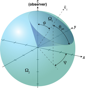
Figure 8. SUBLIME model geometry used in the present study showing the conical jet (Ω1) and ambient coma (Ω2) in Cartesian coordinates. Here θjet is the half-opening angle of the conical jet, ϕ is the (phase) angle of the jet axis with respect to the observer (z), and ψ is the jet position angle in the plane of the sky (x is north, y is east).
Download figure:
Standard image High-resolution imageAppendix B: Interferometric Visibility Spectral Modeling
Figures 9–14 show the real part of the observed and modeled ALMA visibilities for comet 46P as a function of spectral channel. The top panel of each figure shows the autocorrelation (total power) spectrum, while each successive panel shows the data averaged over a range of increasing antenna baseline lengths (corresponding to decreasing angular scales). Figure 15 shows a zoomed, unbinned version of Figure 5 for CH3OH to highlight the difference between the two best-fitting models and the data.
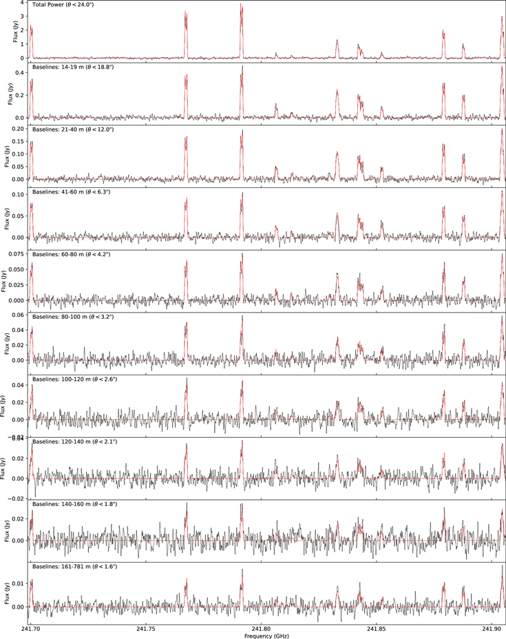
Figure 9. The CH3OH JK = 5K –4K binned visibility spectra (real component) with the best-fitting model overlaid in red. Each panel shows the average spectrum for a range of uv distances (antenna baselines), given in the upper-left corner, which correspond to a range of angular scales (θ) on the sky.
Download figure:
Standard image High-resolution image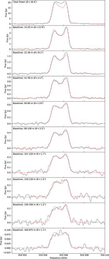
Figure 10. The HCN J = 4–3 binned visibility spectra (real component) with the best-fitting model overlaid in red. Each panel shows the average spectrum for a range of uv distances (antenna baselines), given in the upper-left corner, which correspond to a range of angular scales (θ) on the sky.
Download figure:
Standard image High-resolution image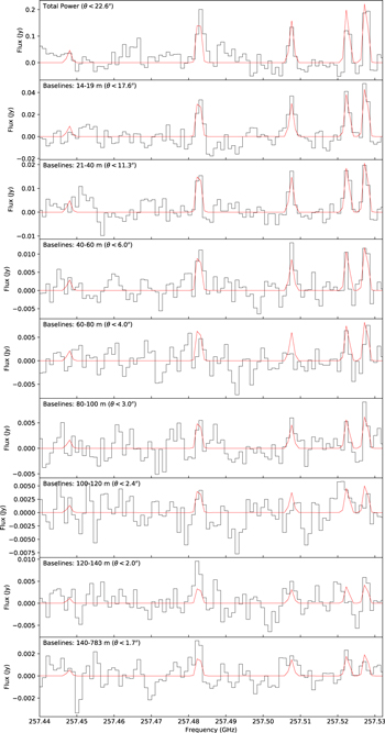
Figure 11. The CH3CN JK = 14K –13K binned visibility spectra (real component) with the best-fitting model overlaid in red. Each panel shows the average spectrum for a range of uv distances (antenna baselines), given in the upper-left corner, which correspond to a range of angular scales (θ) on the sky.
Download figure:
Standard image High-resolution image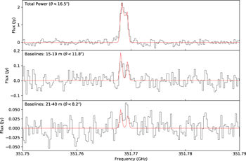
Figure 12. The H2CO  –41,4 binned visibility spectra (real component) with the best-fitting model overlaid in red. Each panel shows the average spectrum for a range of uv distances (antenna baselines), given in the upper-left corner, which correspond to a range of angular scales (θ) on the sky.
Download figure:
Standard image High-resolution image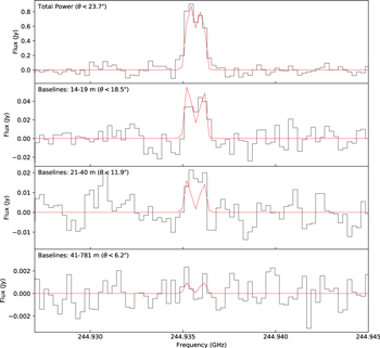
Figure 13. The CS J = 5–4 binned visibility spectra (real component) with the best-fitting model overlaid in red. Each panel shows the average spectrum for a range of uv distances (antenna baselines), given in the upper-left corner, which correspond to a range of angular scales (θ) on the sky.
Download figure:
Standard image High-resolution image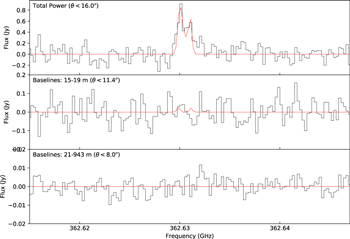
Figure 14. The HNC J = 4–3 binned visibility spectra (real component) with the best-fitting model overlaid in red. Each panel shows the average spectrum for a range of uv distances (antenna baselines), given in the upper-left corner, which correspond to a range of angular scales (θ) on the sky.
Download figure:
Standard image High-resolution image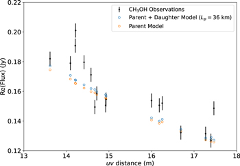
Figure 15. Observed, spectrally averaged real interferometric visibilities for CH3OH zoomed in on the region of shortest baselines to show the improved fit of the parent + daughter model (blue circles) compared with the pure parent model (orange circles).
Download figure:
Standard image High-resolution image