The following article is Open access

Global Chemical Transport on Hot Jupiters: Insights from the 2D VULCAN Photochemical Model

Shang-Min Tsai, Vivien Parmentier, João M. Mendonça, Xianyu Tan, Russell Deitrick, Mark Hammond, Arjun B. Savel, Xi Zhang, Raymond T. Pierrehumbert, and Edward W. Schwieterman

Published 2024 February 27 • © 2024. The Author(s). Published by the American Astronomical Society.
The Astrophysical Journal, Volume 963, Number 1Citation Shang-Min Tsai et al 2024 ApJ 963 41DOI 10.3847/1538-4357/ad1600

Download Article PDF

DownloadArticle ePub

You need an eReader or compatible software to experience the benefits of the ePub3 file format.

Article metrics

1113 Total downloads
0 Video abstract views

Dates

Received 2023 October 21
Revised 2023 November 29
Accepted 2023 December 13
Published 2024 February 27

Unified Astronomy Thesaurus concepts

Exoplanet atmospheres; Exoplanet atmospheric composition; Exoplanet atmospheric dynamics; Planetary atmospheres

Journal RSS

Create or edit your corridor alerts

What are corridors?

Abstract

The atmospheric dynamics of tidally locked hot Jupiters is characterized by strong equatorial winds. Understanding the interaction between global circulation and chemistry is crucial in atmospheric studies and interpreting observations. Two-dimensional (2D) photochemical transport models shed light on how the atmospheric composition depends on circulation. In this paper, we introduce the 2D photochemical (horizontal and vertical) transport model, VULCAN 2D, which improves on the pseudo-2D approaches by allowing for nonuniform zonal winds. We extensively validate our VULCAN 2D with analytical solutions and benchmark comparisons. Applications to HD 189733 b and HD 209458 b reveal a transition in mixing regimes: horizontal transport predominates below ∼0.1 mbar, while vertical mixing is more important at higher altitudes above 0.1 mbar. Motivated by the previously inferred carbon-rich atmosphere, we find that HD 209458 b with supersolar carbon-to-oxygen ratio (C/O) exhibits pronounced C₂H₄ absorption on the morning limb but not on the evening limb, due to horizontal transport from the nightside. We discuss when a pseudo-2D approach is a valid assumption and its inherent limitations. Finally, we demonstrate the effect of horizontal transport in transmission observations and its impact on the morning−evening limb asymmetry with synthetic spectra, highlighting the need to consider global transport when interpreting exoplanet atmospheres.

Export citation and abstractBibTeX RIS

Previous article in issue

Next article in issue

Original content from this work may be used under the terms of the Creative Commons Attribution 4.0 licence. Any further distribution of this work must maintain attribution to the author(s) and the title of the work, journal citation and DOI.

1. Introduction

We are entering the era of detailed exoplanet atmosphere characterization. The atmospheric characterization has come a long way since the first transit observation with the Hubble Space Telescope (HST; Charbonneau et al. 2002). Recent JWST spectral measurements revealed unprecedented details of gas giants (e.g., Bell et al. 2023; JWST Transiting Exoplanet Community Early Release Science Team et al. 2023; Rustamkulov et al. 2023). Transmission spectroscopy is central for probing atmospheric composition. To improve our ability to interpret observations through theoretical models, it is important to consider how the temperature and composition at the terminators and various regions are shaped by global circulation. This aspect cannot be addressed by traditional 1D models that omit thermal and chemical variations and transport processes in the horizontal direction.

Since transmission observations probe terminator regions that are composed of opposite sides of the planet, recent works have highlighted the need to account for spatial inhomogeneities. Espinoza & Jones (2021) and Grant & Wakeford (2023) introduced methods to separate the atmospheric components from the morning (leading) and evening (trailing) limbs. The advancement of high-resolution spectroscopy also expands our capacity to resolve the climate (e.g., Louden & Wheatley 2015) and chemical variations (e.g., Ehrenreich et al. 2020; Wardenier et al. 2021) across the planet. Atmospheric retrieval frameworks are beginning to extend to 2D and 3D to prevent biases from fitting the data with 1D profiles (MacDonald et al. 2020; Chubb & Min 2022; Pluriel et al. 2022). As we gain more complete observations from transit, eclipse, and phase curves, we will soon have the ability to probe the composition distributions across the planet. It is essential to have models resolving global variations to support the progress of observations.

The atmospheric composition of gas giants is generally governed by thermochemistry, photochemistry, and mixing processes. The merit of 1D models is that they can incorporate all the above processes as needed. However, the 1D structure intrinsically neglects the variations in 3D and, more importantly, how the global circulation impacts the local properties (Mendonça et al. 2018a; Drummond et al. 2020; Zamyatina et al. 2023). 3D general circulation models (GCMs) can capture the intricate dynamic interactions across the planet and have become commonly applied to interpret observations (e.g., Beltz et al. 2021; Kempton et al. 2023). However, simplifications of the physical and chemical processes are usually required owing to computation limitations. In addition to reducing the full Navier–Stokes dynamics into primitive equations (Mayne et al. 2019), 3D GCMs often make further simplifications to radiative transfer and chemical processes. The chemical processes in particular are often severely simplified in most applications, using the assumption of thermochemical equilibrium, which is valid only at high temperatures and pressures. Modeling efforts have been put into implementing reduced chemical schemes in a GCM to account for transport-induced disequilibrium (Drummond et al. 2020; Tsai et al. 2022; Lee et al. 2023). While Earth climate models have provided insights into the oxygen response of Earth-like atmospheres (Chen et al. 2021; Cooke et al. 2022; Braam et al. 2023; Deitrick & Goldblatt 2023; Ji et al. 2023), to date the incorporation of photochemistry into 3D models for diverse non-Earth-like atmospheres has not yet been realized.

For most tidally locked giant exoplanets, the stationary day–night heating drives large-scale equatorial waves. These waves interact with background flows and transport momentum from higher latitudes toward the equator, leading to an equatorial superrotating jet (Showman & Polvani 2011; Tsai et al. 2014; Showman et al. 2020). The strong jet plays a central role in global circulation, facilitating the transport of heat, aerosols, and gaseous species (Komacek & Showman 2016; Drummond et al. 2020; Hammond & Lewis 2021; Steinrueck et al. 2021). For these planets, “pseudo-2D” photochemical models (Agúndez et al. 2014; Venot et al. 2020; Baeyens et al. 2022; Moses et al. 2022) that employ a rotating 1D column to mimic a uniform jet in a Lagrangian frame have emerged as useful complementary tools. Their relatively fast computation enables them to incorporate the same detailed mechanisms as 1D models, but the simulated circulation is limited to uniform winds.¹¹ On the other hand, 2D models implemented with horizontal diffusion have been used to model the meridional plane for solar system gas giants (Liang et al. 2005; Zhang et al. 2013; Hue et al. 2018) but have not yet been applied to exoplanets. In this work, we present the 2D (horizontal and vertical) photochemical transport model VULCAN 2D, which lifts this restriction on wind patterns while sharing the same advantage as pseudo-2D models. While VULCAN 2D is constructed with horizontal and vertical dimensions in general, here we will focus on the zonal and vertical directions.

In Section 2, we describe the construction of the VULCAN 2D model. In Section 3, we validate the numerical scheme and modeling results through comparisons to an analytical solution, a pseudo-2D approach, and a 3D GCM. In Section 4, we delve into the applications to canonical hot Jupiters, HD 189733 b and HD 209458 b, including a supersolar C/O scenario for HD 209458 b. We use limiting cases to demonstrate the roles of horizontal and vertical transport and draw comparisons with previous works (Agúndez et al. 2014). We then compare VULCAN 2D to pseudo-2D models in Section 5, exploring when the uniform wind assumption in pseudo-2D models may no longer hold. Finally, we discuss the observational implications and the morning−evening limb asymmetry arising from horizontal transport in Section 6.

2. Configuration of the 2D Chemical Transport Model

2.1. The 2D Grid

A standard 1D photochemical kinetics model solves the continuity equation in the form of a set of coupled partial differential equations:

where n is the number density (cm⁻³) of each species and t denotes the time. ${ \mathcal P }$ and ${ \mathcal L }$ are the chemical production and loss rates (cm⁻³ s⁻¹), respectively, of the corresponding species at each vertical layer (Tsai et al. 2017). Equation (1) can be readily generalized to a 2D Cartesian space (x, z) to include horizontal transport:

where ϕ_z and ϕ_x are the vertical (z) and horizontal (x) transport flux, respectively. In general, ϕ_z encompasses vertical advection, eddy diffusion, and molecular diffusion (Tsai et al. 2021), whereas ϕ_x describes horizontal transport on isobaric surfaces. Using isobaric flux is motivated by the fact that previous analysis of 3D GCMs is traditionally done in isobaric coordinates and that winds on the isobaric levels typically dominate heat and chemical transport on tidally locked planets (e.g., Koll & Komacek 2018; Showman et al. 2020; Hammond & Lewis 2021). We note that we use log-pressure coordinates, with the vertical coordinate defined as $z=-H\ {\rm{ln}}(p/{P}_{s})$ , where H is the pressure scale height that depends on the local temperature, mean molecular weight, and altitude-dependent gravity and P_s is the reference pressure. While each vertical column uses the same pressure grid spaced uniformly in log-space, the corresponding z differs between columns owing to the horizontal temperature gradient. Therefore, the horizontal derivative is evaluated at the same pressure level but not the same geometric height. The configuration of our 2D grid is illustrated in Figure 1.

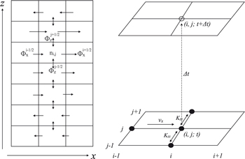
Figure 1. Refer to the following caption and surrounding text. — **Figure 1.** The grid configuration of VULCAN 2D (left) and the stencil of the upwind scheme for horizontal (i) advection and vertical (j) diffusion (right). The arrows illustrate the advection and diffusion transport between adjacent grids.
Download figure:
Standard image High-resolution image

The real challenge lies in numerically solving Equation (2). Most of the numerical methods for stiff equations require evaluating the Jacobian matrix (Brasseur & Jacob 2017). In a 1D system, the Jacobian matrix is neatly constructed through nested looping each species within each vertical layer (see Figure 14 in Tsai et al. 2017). For example, the Rosenbrock method with a band matrix solver is employed in VULCAN. However, this structure breaks down when extending to 2D. To take advantage of the established numerical solver built for 1D systems, we apply an asynchronous integrator within each time step (Small et al. 2013). Specifically, the right-hand side of Equation (2) is first discretized in x as

where i and j denote the vertical and horizontal indices, respectively, and +1/2 and −1/2 represent the interfaces enclosing that layer. Equation (3) is evaluated for each species and each vertical column. Since the last term (i.e., the horizontal transport flux) on the right-hand side of Equation (3) only contributes to the diagonal elements in the Jacobian matrix, Equation (3) has the same numerical structure as that in a 1D system (Equation (5) in Tsai et al. 2017). This allows us to evaluate each column, including horizontal transport, using the existing 1D solver. Specifically, Equation (3) is computed for each x column within each time step. Although errors can arise from the asynchronous update of horizontal transport flux associated with each column, we have tested integrating each column in different orders and found the errors to be negligible.

For the horizontal advection, we adopt a first-order upwind difference scheme, where the local concentration is affected by the upwind cell only (same as the vertical advection described in Tsai et al. 2021). The advective flux for the k cell in the x-direction is

where v_k−1/2 and v_k+1/2 are the zonal wind velocities at the left and right interfaces of the grid cell k, respectively. In addition to advective transport, horizontal diffusion contributes to meridional transport on Jupiter and Saturn (Zhang et al. 2013; Hue et al. 2015, 2018) and is also implemented in VULCAN 2D. However, as horizontal winds can be directly obtained from GCM output, we focus only on advection for horizontal transport and diffusion for vertical mixing in this study.

The advantage of our 2D spatial grid is that it accommodates nonuniform 2D flow patterns, such as the mean meridional or zonal circulation derived from the 3D GCM. In contrast, for pseudo-2D models that employ a Lagrangian rotating 1D column (Agúndez et al. 2014), the horizontal transport is restricted to a uniform jet by design. Both our 2D model and the pseudo-2D model share a limitation known as the Courant–Friedrichs–Lewy (CFL) condition (Courant et al. 1928), as already pointed out by Zhang et al. (2013). Given that we explicitly solve for each vertical column, the integration step size must be constrained by the time it takes for the horizontal flow to travel to neighboring grid cells. This constraint becomes more stringent as the number of horizontal columns increases. In practice, to reduce the overall integration time to achieve convergence, we initially run our 2D model without horizontal transport (thereby removing the step-size restriction) to attain the 1D steady state. We then run the full 2D VULCAN from this steady state (achieved without horizontal transport) with the step size limited by the CFL condition: ${dt}\lt \min \left(\tfrac{{dx}}{{v}_{x}}\right)$ until the final steady state. Current VULCAN 2D evaluates each vertical column in sequence. Therefore, the simulation runtime scales with the number of columns linearly. However, there are opportunities to enhance code efficiency with parallel integration across the horizontal domain. Future development of VULCAN 2D will explore multiprocessing to speed up column-based computations.

3. Validation and Comparison to Previous Work

3.1. Validation with Analytical Solutions

Zhang et al. (2013) derived an analytical solution for a 2D advective−diffusive system with parameterized chemical sources and sinks. We apply their analytical solution for a 2D zonal plane to validate our numerical model. To briefly recap, Equation (13) in Zhang et al. (2013) describes the steady-state abundance as a function of longitude and altitude, governed by vertical diffusion, horizontal advection, and chemical sources and sinks. We assume vertically uniform diffusion to simplify the expression, i.e., with α = γ = 0, the analytical solution for the volume mixing ratio under day–night sinusoidal chemical production (k = 1) is

where χ is the volume mixing ratio, λ is longitude, ϕ is the phase shift, ξ is the vertical coordinate, P₀ and L₀ are the production and loss rates, respectively, and q relates the ratio of advection to chemical timescales, following the same notation as in Zhang et al. (2013).

To compare with the analytical solution, we implemented a mock chemical network with only A and B as reactive species. The rate constant of A → B is given by L₀ N₀ e^−ξ/[A], and that of B → A is given by ${P}_{0}{N}_{0}(1+{\rm{\cos }}k\lambda )$ /[B], corresponding to the loss and production prescriptions in Section 5 of Zhang et al. (2013). We assume constant zonal winds of 71.5 m s⁻¹ and R_p = R_J, together with P₀ N₀ = 2 × 10⁻⁷ cm⁻³ s⁻¹ and L₀ N₀ = 2 × 10⁻⁷ cm⁻³ s⁻¹, to yield q = 1. The vertical diffusion is set to 10⁸ cm⁻² s⁻¹, but the horizontal distribution does not directly depend on this value.

Figure 2 compares our 2D numerical model to the analytical solution. The impact of the horizontal wind is twofold: it both transports and homogenizes the chemical gradient. While our numerical results show somewhat lower peak amplitudes than the analytical solution, which can likely be attributed to numerical diffusion, they effectively capture the overall distribution shape and correctly reproduce the “phase shift” due to eastward transport.

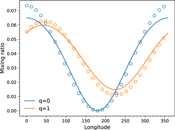
Figure 2. Refer to the following caption and surrounding text. — **Figure 2.** Comparison of VULCAN 2D (solid curve) to analytical solutions (open circles), showing the volume mixing ratio at ξ = 1 with q = 0 (no zonal transport) and q = 1 (eastward zonal transport). The q = 1 case represents zonal transport on a timescale comparable to the chemical timescale.
Download figure:
Standard image High-resolution image

3.2. Comparison with the Pseudo-2D Approach (Agúndez et al. 2014)

Agúndez et al. (2014) apply a rotating 1D model to represent an air column moving with a uniform zonal jet in a Lagrangian frame. Their chemical kinetics scheme was based on Venot et al. (2012). For a like-for-like comparison, we adopt the same rotating 1D column as Agúndez et al. (2014; referred to as Lagrangian-1D VULCAN) and compare it against our 2D photochemical model (2D VULCAN) using the identical N–C–H–O chemical scheme in VULCAN. We chose the canonical hot Jupiter HD 189733 b for this comparison, employing the same GCM output as that in Agúndez et al. (2014). In Lagrangian-1D VULCAN, the 1D column is set to travel around the equator over 2.435 days, following Agúndez et al. (2014), i.e., with a constant angular velocity of 1.493 × 10⁻⁵ rad s⁻¹. To translate this rotation into the equivalent zonal-mean wind, we use a quasi-uniform zonal wind (faster at higher altitudes) in 2D VULCAN to match the same angular velocity. The zonal wind is 2430 m s⁻¹ at 1 bar and scaled to each altitude according to the geometry. The equatorial plane is divided into 64 columns in longitude for both 2D VULCAN and Lagrangian-1D VULCAN. We used the same eddy diffusion coefficient (K_zz) for vertical mixing as Agúndez et al. (2014): K_zz = 10⁷ × (P/1 bar)^−0.65 cm² s⁻¹. Other physical and chemical parameters were kept as much the same as possible between Lagrangian-1D and 2D VULCAN models.

The comparisons between our Lagrangian-1D VULCAN and 2D VULCAN for species displaying apparent longitudinal gradients are shown in Figure 3. 2D VULCAN and Lagrangian-1D VULCAN exhibit consistent results for species with either short (e.g., H) or long (e.g., CH₄) chemical timescales. This indicates that 2D VULCAN correctly captures the processes of vertical mixing and horizontal transport. We find minor deviations that appeared in trace species (volume mixing ratios ≲10⁻⁶). For instance, NH₃ exhibits the most notable differences above 10⁻⁴ bar. The discrepancy is likely due to the numerical integration: the first-order upwind in 2D VULCAN has stronger numerical diffusion than the Rosenberg method with second-order convergence in time used in Lagrangian-1D VULCAN. Nevertheless, the agreements are generally within a factor of two in the region below 0.1 mbar level. Our 2D VULCAN, with the equivalent uniform wind, can successfully reproduce the results obtained by the Lagrangian-1D approach.

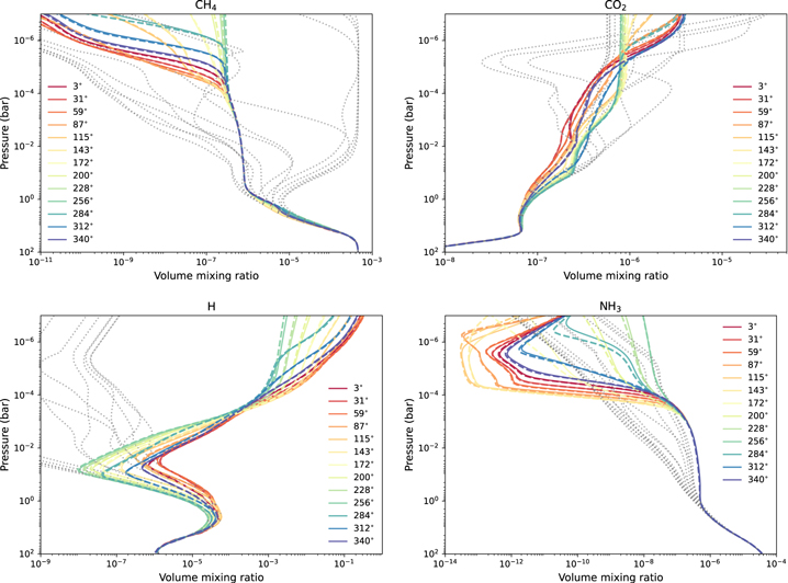
Figure 3. Refer to the following caption and surrounding text. — **Figure 3.** Mixing ratio profiles at various longitudes of HD 189733 b using Lagrangian-1D VULCAN (dashed) compared to those using 2D VULCAN with equivalent zonal winds (solid; see text for details). The substellar point is at 0° longitude. Lagrangian-1D VULCAN has the same configuration as the pseudo-2D model (e.g., Agúndez et al. 2014; Baeyens et al. 2021). Equilibrium abundances are indicated by the gray lines.
Download figure:
Standard image High-resolution image

3.3. Comparison with 3D Transport (without Photochemistry)

We have validated VULCAN 2D through an analytical solution and a pseudo-2D approach, to ensure the accuracy of our physical and numerical implementation within the 2D framework. In our next step, we will perform additional comparisons with a 3D GCM to see whether our 2D model effectively captures the primary transport process.

Mendonça et al. (2018b) previously investigated the global transport of chemically active tracers: H₂O, CH₄, CO, and CO₂ in the 3D simulation of WASP-43 b. The chemical relaxation scheme (Tsai et al. 2018) implemented in Mendonça et al. (2018b) simplifies the thermochemical kinetics with a linear response according to the chemical timescale. We compare with the work by Mendonça et al. (2018b) because their chemical timescales are derived from the same chemical network implemented in VULCAN. Here photochemistry in 2D VULCAN is switched off to have an equivalent comparison. The equatorial region (±20°) is divided into four quadrants in longitude: dayside (315°–45°), morning limb (225°–315°), nightside (135°–225°), and evening limb (45°–135°), following Figure 4 in Mendonça et al. (2018b). We adopt the average temperature and zonal wind field in this equatorial region from the same GCM output in Mendonça et al. (2018a, 2018b). The eddy diffusion coefficients are often estimated from mixing-length theory, using rms vertical velocity (w_rms) as the turbulent velocity and the scale height (H) as the mixing length. However, Parmentier et al. (2013) demonstrated that this approach tends to overestimate vertical mixing efficiency for hot Jupiters. Given this likely overestimation, we make two assumptions, K_zz = w_rms H and K_zz = 0.01 × w_rms H, to bracket the plausible range of K_zz. The average temperature from the GCM is used to compute the scale height $H=\tfrac{{k}_{{\rm{B}}}T}{{mg}}$ (k_B: Boltzmann constant; g: altitude-dependent gravitational acceleration), but we fix the mean molecular weight m to 2.2387, following the same setting as in Mendonça et al. (2018a, 2018b).

Figure 4 compares the abundance distribution of CH₄ (for solar composition) and H₂O (for C/O = 2) in the four quadrants of the equatorial region computed by VULCAN 2D and Mendonça et al. (2018a). Our 2D model with K_zz = 0.01 × w_rms H predicts vertical quench levels close to those in the 3D results. The preference for a weaker K_zz might be attributed to the high gravity of WASP-43 b. The slight increase of H₂O between 0.1 and 0.01 in the 3D GCM is likely associated with meridional transport from higher latitude (Drummond et al. 2018) not accounted for in the 2D model. The overall good agreement between VULCAN 2D and the 3D results reinforces our 2D model’s representation of the mixing process in the equatorial region of a hot Jupiter.

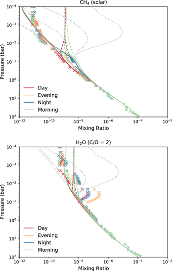
Figure 4. Refer to the following caption and surrounding text. — **Figure 4.** CH₄ (top) and H₂O (bottom) abundances computed by VULCAN 2D for WASP-43 b compared to those in Mendonça et al. (2018b) (crosses), showing the averaged mixing ratio profiles with eddy diffusion K_zz = 0.01 × w_rms H (solid) and K_zz = w_rms H (dashed) on the dayside (315°–45°), morning limb (225°–315°), nightside (135°–225°), and evening limb (45°–135°). We present the cases that exhibit the most compositional gradient: CH₄ from the solar composition simulation and H₂O from the C/O = 2 simulation. The resulting distribution profiles with K_zz = 0.01 × w_rms H better represent those from the 3D GCM.
Download figure:
Standard image High-resolution image

4. Results: Equatorial Chemical Distributions on HD 189733 b and HD 209458 b

We now first present an overview of the abundance distribution in the atmosphere of our fiducial simulations of HD 189733 b and HD 2094598 b. We briefly compare our results to previous work by Agúndez et al. (2014) on the same planets. To gain insight into the effects of vertical and horizontal transport, we examine the limiting cases where individual transport processes are isolated following the approach of Agúndez et al. (2014). We then explore the sensitivity to the eddy diffusion coefficients converted from the GCM wind and discuss the results guided by the limiting cases. Lastly, we explore the global chemical transport when C/O ≳ 1 with HD 209458 b, motivated by recent high spectral resolution observations.

4.1. Setup and Overview

We adopt 3D GCM output from SPARC/MITgcm (Adcroft et al. 2004; Showman et al. 2009) for HD 189733 b and HD 209458 b. Chemical equilibrium is assumed when calculating radiative transfer with the correlated-k distribution method. For HD 189733 b, we use the same GCM output as Agúndez et al. (2014), where detailed GCM parameters are further listed in Table 1 of Steinrueck et al. (2019). For HD 209458 b, we do not include TiO and VO as shortwave opacity sources in our simulation, based on the lack of evidence of a thermal inversion from the reanalysis of emission spectra obtained by Spitzer and HST (Diamond-Lowe et al. 2014; Line et al. 2016). The parameters for our HD 209458 b GCM can be found in Parmentier et al. (2013), with the change that TiO and VO opacities have been removed. The lower and upper pressure boundaries of the GCM simulations are 200 bar and 2 × 10⁻⁶ bar, respectively. To extend the model domain for VULCAN 2D, the temperatures and winds at the upper GCM boundary are held constant up to 10⁻⁸ bar.

The equatorial average temperatures and winds for our HD 189733 b and HD 209458 b simulations are shown in Figure 5. The zonal wind speeds evidently vary across longitudes at pressures above 0.1 bar. Both planets share similar thermal and dynamical structures in the equatorial region, though HD 209458 b exhibits higher temperatures and overall faster zonal wind speeds. We adopt the same global eddy diffusion coefficients as Agúndez et al. (2014) for vertical mixing. These K_zz profiles are compared with those estimated by the mixing-length theory in Figure 21. We will further explore the sensitivity to the adopted eddy diffusion coefficients in Section 4.4. For VULCAN 2D, we apply the N–C–H–O chemical network¹² and omit sulfur throughout this study.

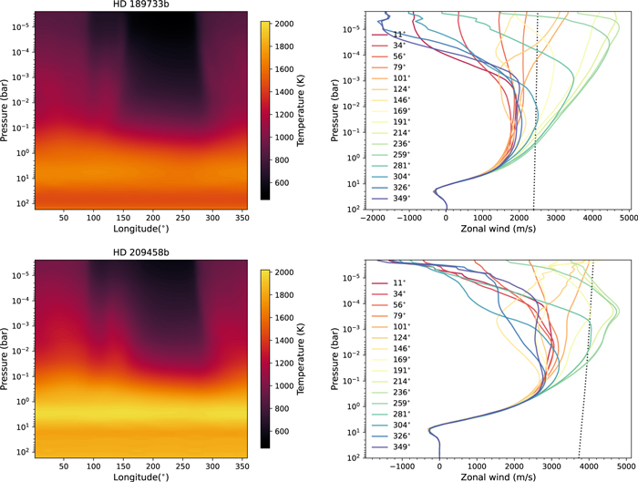
Figure 5. Refer to the following caption and surrounding text. — **Figure 5.** The equatorial temperature (left) and zonal winds (right) from our GCMs of HD 209458 b and HD 189733 b, averaged over ±30° latitudes. The substellar point is located at 0° longitude. The uniform zonal winds (constant angular velocities with 2430 m s⁻¹ for HD 189733 b and 3850 m s⁻¹ for HD 209458 b at the 1 bar pressure level, respectively) assumed in Agúndez et al. (2014) are illustrated with black dotted lines in the right panels for comparison.
Download figure:
Standard image High-resolution image

Figures 6 and 7 showcase the chemical abundance distributions simulated by VULCAN 2D in the equatorial regions of HD 189733 b and HD 209458 b. The vertical abundance distributions along longitudes of several important species are summarized in Figure 8. In the observable regions of the atmospheres, species such as CH₄, H, NH₃, and HCN show considerable horizontal (longitudinal) gradient, whereas H₂O and CO (not shown) are rather uniform everywhere. The uniformity is expected since the equilibrium abundances of H₂O and CO do not vary with longitude in the first place. Species that are more susceptible to photodissociation, such as CH₄ and NH₃, are destroyed on the dayside but can partly recover on the nightside. Photochemical products, such as atomic H and HCN, build up on the dayside while being transported horizontally by the zonal jet at the same time. We find that the chemical transport exhibits qualitative similarities between HD 189733 b and HD 209458 b, with the main difference being that CH₄ and NH₃ are more favored on the cooler HD 189733 b.

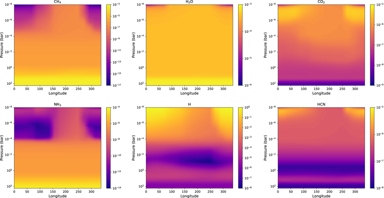
Figure 6. Refer to the following caption and surrounding text. — **Figure 6.** The equatorial abundance distribution (in color contours) of several chemical species as a function of longitude and pressure on HD 189733 b. The substellar point is located at 0° longitude.
Download figure:
Standard image High-resolution image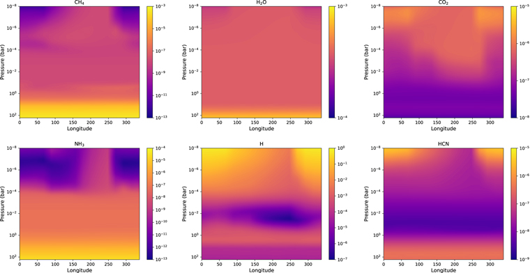

Figure 7. Refer to the following caption and surrounding text. — **Figure 7.** Same as Figure 6, but for HD 209458 b.
Download figure:
Standard image High-resolution image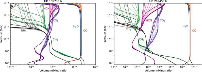

Figure 8. Refer to the following caption and surrounding text. — **Figure 8.** The vertical profiles in the equatorial regions of HD 189733 b and HD 209458 b simulated by 2D VULCAN. The shades of colors from light to dark correspond to longitudes from the substellar point (0°) through nightside and back around to the substellar point (360°).
Download figure:
Standard image High-resolution image

This behavior of chemical transport can be understood by comparing the horizontal and vertical dynamical timescales, as illustrated in Figure 10: horizontal mixing dominates at altitudes below ∼0.1 mbar, while vertical mixing dominates at altitudes above ∼0.1 mbar. Within the horizontal mixing region, species with longer timescales tend to display more uniform global abundances, whereas compositional gradients in the upper atmosphere are mainly controlled by vertical mixing and photochemistry.

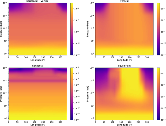
Figure 9. Refer to the following caption and surrounding text. — **Figure 9.** The equatorial distribution of CH₄ as a function of longitude and pressure on HD 189733 b, from our nominal model, vertical mixing model, horizontal transport model, and chemical equilibrium. Note that the color bars have different scales.
Download figure:
Standard image High-resolution image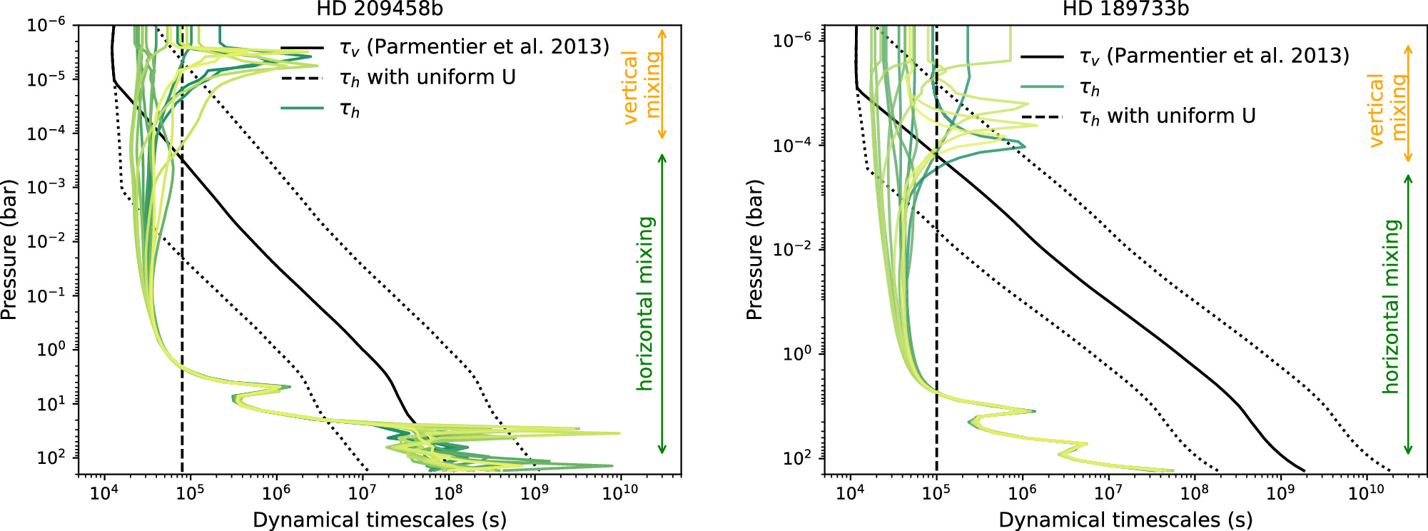

Figure 10. Refer to the following caption and surrounding text. — **Figure 10.** The dynamical timescales of vertical transport (τ_v) and horizontal transport (τ_h). The black dotted lines indicate the vertical transport timescale with 10 times and 0.1 times eddy diffusion coefficients. The horizontal transport timescale at different longitudinal locations is depicted in gradient shades of green, while the uniform horizontal wind assumed in Agúndez et al. (2014) is shown as the dashed lines. The arrows on the right indicate the regions dominated by horizontal transport and vertical transport processes.
Download figure:
Standard image High-resolution image

4.2. Limiting Cases with Only Horizontal Transport and with Only Vertical Mixing

Following the pedagogical exercise in Agúndez et al. (2014), this section presents the simulated vertical abundance profiles of HD 189733 b and HD 209458 b under limiting cases to isolate individual dynamical effects. Specifically, we examine scenarios where we exclude horizontal transport and vertical mixing, respectively. Figures 9 and 11 first show the distributions of CH₄ and H in these limiting cases, demonstrating the principles of horizontal transport and vertical mixing. As expected, vertical mixing tends to homogenize the vertical gradient of composition, while horizontal transport tends to homogenize the horizontal gradient. However, the influence of transport processes on a species depends on its chemical properties, which can be broadly categorized into two groups: For species like CH₄ that are replenished from the deep thermochemical regions, vertical mixing provides a zeroth-order prediction on their abundances. For photochemical products like H that are predominantly produced on the dayside upper atmosphere, horizontal transport is crucial to account for their circulation to the nightside.

Figure 11. Refer to the following caption and surrounding text. — **Figure 11.** Same as Figure 9, but for H.
Download figure:
Standard image High-resolution image

Detailed comparisons between the nominal 2D models, the vertical mixing case, the horizontal transport case, and chemical equilibrium at different longitudinal locations are presented in Figures 12 and 13. Examining the quenched species such as CH₄ and NH₃, we find that the vertical mixing and horizontal transport cases have the same quench levels. This is not surprising, as these quench levels correspond to the transition point associated with the same chemical timescales, regardless of the dynamical process.

Figure 12. Refer to the following caption and surrounding text. — **Figure 12.** The abundance profiles of selected species on HD 189733 b at four longitudes: substellar point, evening limb, antistellar point, and morning limb. The volume mixing ratios computed by the nominal 2D model (solid) are compared to the vertical mixing case (excluding horizontal transport; dashed), the horizontal transport case (excluding vertical diffusion; dashed–dotted), and thermochemical equilibrium (dotted).
Download figure:
Standard image High-resolution image

Figure 13. Refer to the following caption and surrounding text. — **Figure 13.** The abundance profiles of selected species on HD 209458 b at four longitudes: substellar point, evening limb, antistellar point, and morning limb. The volume mixing ratios computed by the nominal 2D model (solid) are compared to the vertical mixing case (excluding horizontal transport; dashed), the horizontal transport case (excluding vertical diffusion; dashed–dotted), and thermochemical equilibrium (dotted).
Download figure:
Standard image High-resolution image

However, the abundance distributions above the quench levels differ substantially between the vertical mixing and horizontal transport scenarios. This is because vertical mixing makes chemical abundances quenched from the hot deep layers, while horizontal transport results in quenching from the hot and irradiated dayside, as also noted in Agúndez et al. (2014). Due to this nature of horizontal transport, the substellar abundance profiles closely resemble those from the vertical mixing case (the close match between the solid and dashed lines) for both planets.

Taking a closer look at Figures 12 and 13, species with long chemical timescales like CH₄ and NH₃ closely follow the vertical mixing distribution at hotter longitudes, the substellar point and evening limb, up to about 10⁻⁴ bar. On the other hand, at the colder antistellar point and morning terminator, the equilibrium abundances differ substantially from the dayside, causing the abundance distribution predicted by the vertical mixing model to diverge from the nominal 2D model (with both vertical and horizontal transport) at these cooler locations. These results shed light on the limitation of applying 1D models to interpret observations that probe the chemical properties of different regions.

One crucial feature of horizontal transport is transporting the photochemical products from the dayside to the nightside (Agúndez et al. 2014; Baeyens et al. 2022). For both planets, atomic H produced by photolysis can penetrate into the nightside, even reaching regions around the antistellar point where no UV photons are available. Transport of atomic H plays a key role in reacting with CH₄ and NH₃ to form HCN on the nightside. The abundances of CH₄ and NH₃ in Figures 12 and 13 fall between those in the vertical mixing and horizontal transport cases, highlighting the importance of considering both mixing processes.

To conclude our limiting-case analysis, we note that for hot Jupiters similar to HD 189733 b and HD 209458 b the 1D model including vertical mixing serves as a fairly good approximation for the dayside. Given that the equatorial jet efficiently transports heat, 1D models generally better capture the hotter evening limb compared to the cooler morning limb in the pressure regions most relevant for transmission spectroscopy. We will discuss the limb asymmetry as a result of horizontal transport more in Sections 4.5.2 and 6.

4.3. Comparison with Agúndez et al. (2014)

There are several differences in modeling assumptions and setups between our models of HD 18933 b and HD 209458 b and those presented in Agúndez et al. (2014): (i) Agúndez et al. (2014) assume uniform zonal winds, while we adopt longitude- and pressure-dependent wind profiles from the GCM; (ii) shortwave opacity sources of TiO and VO, which are responsible for generating thermal inversion, are included in Agúndez et al. (2014) but are not included in our model for HD 209458 b; (iii) Agúndez et al. (2014) use the chemical scheme of Venot et al. (2012), while our study adopts the chemical scheme of Tsai et al. (2021).

Despite these differences, our nominal 2D VULCAN and those from the limiting cases are qualitatively consistent with the pseudo-2D outcomes presented in Agúndez et al. (2014). The major difference lies in the thermal inversion of HD 209458 b in Agúndez et al. (2014), making the dayside temperature at low pressures ∼1000 K higher than that in our model. Consequently, Agúndez et al. (2014) predict lower levels of CH₄, NH₃, and HCN on HD 209458 b. The hotter dayside also leads to a lower equilibrium abundance of CO₂, creating the notable CO₂ day–night contrast seen in Agúndez et al. (2014). Overall, apart from the temperature inversion included in Agúndez et al. (2014), we show qualitative agreements in terms of quenching and transport behaviors. We will discuss the implications of assuming uniform zonal winds (i.e., pseudo-2D model) in Section 5 in more detail.

4.4. Sensitivity to K_zz

While VULCAN has the capability to employ vertical advection instead of eddy diffusion (Tsai et al. 2021), it is numerically more stable to employ diffusion in the vertical direction in conjunction with molecular diffusion. One apparent caveat is that the parameterization of vertical mixing with eddy diffusion has been a long-standing uncertainty in atmospheric modeling (e.g., Smith 1998; Parmentier et al. 2013; Zhang & Showman 2018; Komacek et al. 2019). To test the sensitivity to uncertainties in estimating the eddy diffusion coefficient (K_zz), we vary the eddy diffusion coefficient profile by an order of magnitude in our model of HD 189733 b, both increasing and decreasing it. This explored range roughly spans the uncertain range considered in the previous literature (Smith 1998; Parmentier et al. 2013).

We examine the effects of varying vertical eddy diffusion coefficients on CH₄ and NH₃, the major carbon and nitrogen species that exhibit transport-induced disequilibrium, in Figure 14. Stronger vertical mixing makes the transition to a vertical-mixing-dominated region occur at higher pressures, as expected. This allows morning−evening asymmetries to emerge at somewhat higher pressures when horizontal transport becomes less efficient compared to vertical mixing. The pressure levels where morning−evening asymmetry becomes notable are generally between 1 and 0.05 mbar, as summarized in Table 1. Since the equilibrium abundances of CH₄ and NH₃ monotonically increase with pressure in our HD 189733 b model (see also the discussion in Section 4.3.2 in Tsai et al. 2021 and Fortney et al. 2020), increased vertical mixing also results in slightly higher quenched abundances, while weaker mixing leads to lower abundances from horizontal quenching from the dayside. Other hydrocarbons and HCN also follow similar trends in response to mixing processes to CH₄ and NH₃. Despite these effects, the global distribution of main species only mildly depends on the choice of K_zz within the explored range. For HD 189733 b and HD 209458 b, the bulk of the atmosphere below the millibar level still remains in the horizontal-transport-dominated regime, even when considering strong eddy diffusion.

Table 1. The Pressure Levels (mbar) Where the Morning and Evening Abundances Begin to Deviate by More Than 50%

Species	0.1 × K_zz	Nominal	10 × K_zz
CH₄	0.067	0.14	0.22
NH₃	0.14	0.28	0.57

Download table as: ASCII Typeset image

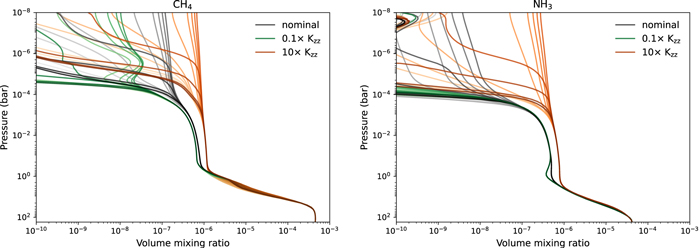
Figure 14. Refer to the following caption and surrounding text. — **Figure 14.** CH₄ and NH₃ vertical profiles in the equatorial regions of HD 189733 b, simulated with 10 times stronger (orange) and weaker (green) eddy diffusion. The shades of colors from light to dark correspond to longitudes from the substellar point (0°) through nightside and back around to the substellar point (360°).
Download figure:
Standard image High-resolution image

4.5. Supersolar C/O of HD 209458 b

4.5.1. Background

The transit observations using high-resolution spectroscopy of HD 209458 b reported detection of H₂O, CO, HCN, CH₄, NH₃, and C₂H₂ molecules at statistically significant levels (Giacobbe et al. 2021). Notably, the presence of CH₄, C₂H₂, and HCN is indicative of supersolar carbon-to-oxygen ratio (C/O), consistent with the previous high-resolution analysis that also detected HCN (Hawker et al. 2018). In contrast, recent JWST/NIRCam transmission spectra of this planet reported nondetections of CH₄, HCN, and C₂H₂ with upper limits provided (Xue et al. 2023), interpreted to have subsolar C/O based on chemical equilibrium.

While the interpretation by Giacobbe et al. (2021) is driven by cross-correlating with grids of models also assuming thermochemical equilibrium, CH₄ is influenced by quenching, while C₂H₂ and HCN can be efficiently produced by photochemistry out of equilibrium. In addition to the nominal HD 209458 b model with solar metallicity and C/O presented in this section, we run a 2D VULCAN model for HD 209458 b with supersolar C/O to explore the chemical transport under the alternative scenario of a carbon-rich atmosphere. We follow the best-fit C/O value of 1.05 as determined by Giacobbe et al. (2021) and keep the same solar metallicity for comparison with our nominal model, since metallicity is not well constrained in Giacobbe et al. (2021).

4.5.2. Enhanced Hydrocarbon and Horizontal-transport-induced Limb Asymmetry

The top and middle panels of Figure 15 depict the same mixing ratio distributions as in Figure 8 but for C/O = 1.05. When C/O exceeds unity, H₂O loses its dominance to CH₄ owing to the lack of available oxygen after CO (Madhusudhan 2012; Moses et al. 2013; Heng et al. 2016). What is intriguing is the production of water resulting from the photolysis of CO in the dayside upper atmosphere above 0.1 mbar. The same process also operates in a solar C/O condition (Moses et al. 2011), but the increase of H₂O is more pronounced here, due to its lower equilibrium composition. Compared to solar C/O, C₂H₂ abundances are significantly enhanced. Moreover, C₂H₂ exhibits substantial zonal variations, spanning several orders of magnitude across the equator between the 1 bar and 0.1 mbar level (bottom panel of Figure 15).

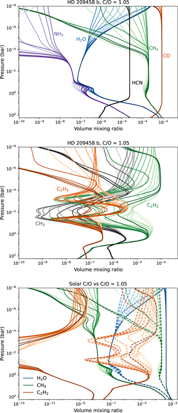
Figure 15. Refer to the following caption and surrounding text. — **Figure 15.** The top and middle panels show the vertical profiles in the equatorial regions as in Figure 8, but for HD 209458 b with C/O = 1.05. The bottom panel compares the key abundance distributions between solar C/O (solid; with C/O ≃ 0.45) and C/O = 1.05 (dashed).
Download figure:
Standard image High-resolution image

Although CH₄ is rather uniform below 10⁻⁴ bar across the planet, several hydrocarbons show notable compositional gradients in the zonal direction, as seen in Figures 15 and 16. C₂H₂ abundance on the evening limb is about 100–1000 times higher than that on the morning limb, whereas C₂H₄ peaks between 0.1 and 10⁻³ bar on the morning limb with strong vertical variations. The morning−evening limb asymmetry in C₂H₂ is driven by the temperature difference and manifested as a result of its relatively short chemical timescale. C₂H₂ is favored at the hotter evening limb, where the temperature is about 200–300 K higher than at the morning limb, as evident in the profiles without zonal wind in Figure 16. In this region, the main destruction pathway for C₂H₂ proceeds through a sequence of unsaturated hydrocarbons:

The timescale of C₂H₂ can be estimated from the rate-limiting steps, the formation of either CH₃ or C₂H₃ in the above pathway. At 1 mbar pressure level, the lifetime of C₂H₂ on the nightside ranges from 10³ to 10⁵ s. This timescale is comparable to that of horizontal transport (Figure 10), explaining the longitudinal compositional gradient C₂H₂ displays.

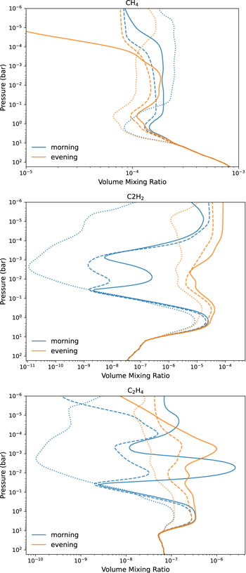
Figure 16. Refer to the following caption and surrounding text. — **Figure 16.** The vertical profiles of CH₄, C₂H₂, and C₂H₄ on the morning and evening limbs in our 2D model of HD 209458 b with C/O = 1.05. The distributions without zonal wind are shown with dashed lines, while chemical equilibrium abundances are indicated by dotted lines.
Download figure:
Standard image High-resolution image

Although C₂H₄ also has a higher equilibrium abundance on the warming evening limb, photochemistry and horizontal transport lead to an accumulation of C₂H₄ on the cooler morning limb instead. The combining effects result in a peak C₂H₄ distribution on the morning limb greater than the abundance on the evening limb, in contrast with the lower morning C₂H₄ abundance predicted in the absence of zonal transport (bottom panel of Figure 16). The photolysis of CH₄ on the dayside produced methyl radical (CH₃), the precursor to produce other hydrocarbons. CH₃ flows into the nightside, where the lower temperature promotes the formation of C₂H₆, C₂H₅, and C₂H₄, since the combination of CH₃ into C₂H₆ is exothermic and kinetically favored at cooler temperatures. With the aid of horizontal transport, the photochemically produced CH₃ is able to transport to the nightside to initiate the production of hydrocarbon species. This hydrocarbon production on the nightside is then carried to the morning limb by the zonal wind, leading to the peak shown in C₂H₄. Similar behavior is found in C₂H₆ distribution as well, but at significantly lower abundances. For completeness, the equatorial abundance distribution as a function of the longitude and pressure of several key species can be found in Figure 22.

5. When Does the Assumption of a Uniform Zonal Jet in Pseudo-2D Models Break Down?

The equatorial jet is a robust feature for tidally locked planets that receive steady day–night thermal forcing (Heng 2015; Showman et al. 2020). However, the equatorial jet transitions to a day-to-night flow when the radiative timescale or drag timescale becomes short (Showman et al. 2015; Komacek et al. 2019). In the case of cooler sub-Neptunes or nonsynchronously rotating planets, the zonal wind in the equatorial region can also develop a more complex structure with winds changing directions across varying pressure levels (Showman et al. 2015; Carone et al. 2020; Charnay et al. 2020; Innes & Pierrehumbert 2022). Here we examine how horizontal transport changes on a hot Jupiter with strong frictional drag dominated by a day-to-night flow. We adopted the output of T_eq = 1600 K with strong drag (τ = 10⁴ s) from Tan & Komacek (2019) as our fiducial atmosphere with a day-to-night flow. The equatorial thermal and wind structures of our fiducial day-to-night circulation and those of HD 189733 b are compared in Figure 23. Our goal is to determine when a pseudo-2D approach with uniform flow remains valid and when it breaks down.

5.1. Comparisons within the Superrotating Regime

The equatorial jets induced by the stationary day–night heating in our HD 189733 b and HD 209458 b models resemble Gaussian-like vertical profiles, gradually diminishing toward zero in both the upper and deeper layers of the atmosphere, as depicted in Figure 5. We use HD 189733 b as an example of circulation characterized by equatorial superrotation for the comparison between 2D and pseudo-2D approaches. For the uniform zonal wind, the pseudo-2D model needs to adopt either the peak jet speed (Agúndez et al. 2014) or the averaged wind velocity over the jet region (Baeyens et al. 2021). For our pseudo-2D model of HD 189733 b, we adopt a mean zonal wind of 1736 m s⁻¹ at 1 bar from the GCM as the uniform zonal wind.

Figure 17 shows the comparison of CH₄ distributions, demonstrating differences caused by the simplified transport in the pseudo-2D approach versus the 2D model. In the deep region where thermochemical equilibrium holds, the actual wind pattern is not effectively relevant. The CH₄ distribution transitions from a horizontal homogenized regime to a vertical-mixing-dominated regime at the same pressure level around 10⁻⁴ bar in both models. In the upper atmosphere above 10⁻⁴ bar, the pseudo-2D model has slightly slower horizontal transport (Figure 10) and predicts slightly more vertically mixed profiles compared to those in our nominal 2D model, where stronger winds around the 1 mbar level at certain longitudes can alter the distribution. Similar trends are seen in other species as well. Despite these minor differences, we find the pseudo-2D approach to be a valid assumption when a broad superrotation jet is present.

Figure 17. Refer to the following caption and surrounding text. — **Figure 17.** The mixing ratio profiles of CH₄ across different longitudes computed from our nominal HD 189733 b model with pressure- and longitude-dependent zonal winds (solid) and from the pseudo-2D model with uniform zonal winds (dashed). We adopt a mean zonal wind velocity of 1736 m s⁻¹ at 1 bar in the nominal model for the uniform wind speed in the pseudo-2D model, following the same approach as in Agúndez et al. (2014).
Download figure:
Standard image High-resolution image

5.2. Comparisons within the Day-to-night Flow Regime

Next, we explore the scenario of a hotter hot Jupiter with strong radiative (e.g., Komacek & Showman 2016) or magnetic drag (e.g., Perna et al. 2010), where the global circulation has changed from equatorial superrotation to day-to-night flow (Miller-Ricci Kempton & Rauscher 2012; Showman et al. 2015; Tan & Komacek 2019). Figure 18 compares the abundance distributions of CH₄ and HCN, the two main molecules that display compositional gradients, in the equatorial region of the fiducial strong-drag hot Jupiter atmosphere with T_eq = 1600 K simulated by our nominal 2D model and pseudo-2D model. It is evident that the day–night flow leads to a symmetrical distribution, differing from the distribution governed by uniform zonal winds. This discrepancy is most pronounced around the morning limb, due to the distinctive transport dynamics at play. In the nominal model, nightside-to-morning-limb advection occurs, contrasting with the morning-limb-to-nightside advection in the model with uniform zonal winds. This circulation pattern also enables more efficient transport of atomic H produced photochemically on the dayside to the morning limb. In the nominal 2D model, the CH₄ and HCN abundances remain low on both morning and evening limbs. Conversely, when assuming uniform eastward winds, CH₄ and HCN exhibit higher abundances around the morning limb owing to nightside transport. Similar to CH₄, species favored on the nightside over the dayside, such as NH₃, follow similar trends, showing higher morning limb abundances in the uniform wind model as well.

Figure 18. Refer to the following caption and surrounding text. — **Figure 18.** The equatorial abundance distribution of CH₄ and HCN. The left column shows the nominal model, and the right column shows the model assuming uniform zonal to simulate the pseudo-2D method. The substellar point is located at 0° longitude.
Download figure:
Standard image High-resolution image

The disparity in abundance profiles across longitudes from the nominal model and pseudo-2D model is further illustrated in Figure 19. Except near the substellar point and at high pressures (P ≳ 1 bar), this comparison demonstrates that for species susceptible to photochemistry the assumption of uniform zonal winds in the pseudo-2D framework can yield orders-of-magnitude differences in the observable region (approximately 0.1 to 10⁻⁵ bar) when the dominant circulation is featured by a day-to-night flow. The pseudo-2D approach is only suitable for a tidally locked atmosphere with moderate drag such that the circulation is still within the equatorial superrotation regime.

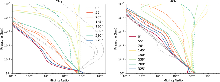
Figure 19. Refer to the following caption and surrounding text. — **Figure 19.** Mixing ratio profiles at several different longitudes in our fiducial ultrahot Jupiter models, with the nominal day-to-night flow (solid), uniform zonal winds (dashed), and chemical equilibrium (gray dotted lines). The pressure domain is zoomed in to the most observable region between 1 and 10⁻⁵ bar for clarity.
Download figure:
Standard image High-resolution image

6. Synthetic Spectra (for the Evening and Morning Limbs)

We present synthetic transmission spectra for the morning and evening limbs based on our 2D model results. The transmission spectra are computed using PLATON (Zhang et al. 2019, 2020), including opacity sources of CH₄, CO, CO₂, C₂H₂, H₂O, HCN, NH₃, O₂, NO, OH, C₂H₄, C₂H₆, H₂CO, and NO₂ and collision-induced absorption (CIA) of H₂–H₂ and H₂–He. We will focus on the observational impact of horizontal transport and the differences between the evening and morning limbs. It is worth noting that the distribution of clouds and hazes can also significantly influence limb asymmetry (Kempton et al. 2017; Powell et al. 2019; Steinrueck et al. 2021; Savel et al. 2023). For the scope of this study, we will leave the effects of clouds to future work and will solely delve into the chemical transport within our cloud-free models.

Figure 20 illustrates the synthetic transmission spectra with and without horizontal transport for HD 189733 b and HD 209458 b (including solar and supersolar C/O). For HD 189733 b, 1D models (i.e., without horizontal transport) produce methane features on the cooler morning limb that are absent on the evening limb (Figure 12). However, this compositional gradient is readily homogenized once the zonal transport is included. For HD 209458 b (solar C/O), methane abundance remains too low in both 1D and 2D models (below ppm level; see Figure 13). Consequently, the influence of horizontal transport on the spectra of HD 209458 b with solar C/O is negligible. Instead, the dominant molecules that show up in the spectra are H₂O, CO, and CO₂, all of which exhibit relatively uniform equilibrium abundances throughout the planet. As a result, these gases do not contribute to limb asymmetry, whether horizontal transport is in play or not. In the case of HD 209458 b with supersolar C/O, CH₄ took over H₂O to make the strongest spectral features at 2.3 μm, 3.3–3.9 μm, 5.5–6.6 μm, and 7–8.5 μm. As CH₄ becomes the predominant carbon-bearing molecule, it also reaches a uniform distribution across the entire planet. The major limb asymmetry is the presence of C₂H₄ absorption on the morning limb but not on the evening limb, due to the horizontal transport of C₂H₄ from the nightside to the morning limb.

Figure 20. Refer to the following caption and surrounding text. — **Figure 20.** The synthetic transmission spectra of the evening and morning limbs of HD 189733 b and HD 209458 b (for both solar and supersolar C/O). The atmospheric structure is derived from MITgcm simulation (Parmentier et al. 2013), with the chemical composition computed by 2D VULCAN. The models excluding zonal transport are also shown for comparison.
Download figure:
Standard image High-resolution image

7. Discussions and Conclusions

In this paper, we present the 2D version of the photochemical model VULCAN. We first validate VULCAN 2D with analytical solutions. VULCAN 2D successfully reproduces the special case equivalent to the pseudo-2D approach with uniform winds and also demonstrates consistent results with a 3D GCM (Mendonça et al. 2018b). We use limiting cases to demonstrate the distinct effects of the vertical and horizontal mixing processes. For canonical hot Jupiters, such as HD 189733 b and HD 209458 b, we find that most of the atmosphere below 1–0.1 mbar is within the horizontal-transport-dominated region, where zonal advection prevails over vertical mixing. In the upper atmosphere above this region, photochemistry and vertical mixing control the composition. We explore the sensitivity to the parameterization of vertical mixing and find a mild dependence in the abundance distribution of our hot Jupiter models. We note that stronger vertical mixing can, in principle, promote morning−evening asymmetry.

For HD 189733 b, the morning−evening limb asymmetry in CH₄ predicted by 1D models is readily homogenized when horizontal transport is included. For HD 209458 b with solar C/O, the transmission spectra exhibit no limb asymmetry attributed to the composition owing to the paucity of CH₄. However, with supersolar C/O, horizontal transport results in notable limb asymmetries in hydrocarbons (C₂H₄ in this case). For atmospheres with circulation dominated by an equatorial jet, we show that the pseudo-2D (rotation 1D column) approach can reasonably capture the transport, but the assumption of uniform flow breaks down for day-to-night circulations under stronger drag, and pseudo-2D models can yield observable differences (0.1 to 10⁻⁵ bar) orders of magnitude apart, particularly for species susceptible to photochemistry or with inherent compositional gradient in equilibrium.

The 2D modeling framework highlights the need to consider both horizontal and vertical transport when interpreting the compositions from transmission observations probing the limbs. The 2D framework developed here bridges the gap between traditional 1D photochemical kinetics models and 3D GCMs that typically exclude chemical kinetics. Future directions include incorporating sulfur chemistry and applying the model to the meridional plane or tidally locked coordinate (Koll & Abbot 2015) to explore the role of overturning circulation.

In this work, we did not explore the effects of vertical advection. The upward or downward transport can lead to significantly different distributions, as already demonstrated in the ammonia distribution on Jupiter by a 1D model (Tsai et al. 2021). Hammond & Lewis (2021) also showed how slow overturning winds could transport much more heat than fast zonal jets on tidally locked planets with weak temperature gradients. A future model development should represent both of these processes.

By elucidating how the atmosphere composition is regulated by global circulation, this 2D modeling approach will pave the way for self-consistent and more comprehensive models and provide a useful tool to enhance the capacity of 3D GCMs for interpreting observations.

Acknowledgments

Part of this work is supported by the European community through the ERC advanced grant EXOCONDENSE (No. 740963; PI: R. T. Pierrehumbert). S.-M.T. acknowledges support from NASA Exobiology grant No. 80NSSC20K1437 and the University of California, Riverside. X.Z. acknowledges support from the NASA Exoplanet Research grant 80NSSC22K0236 and the NASA Interdisciplinary Consortia for Astrobiology Research (ICAR) grant 80NSSC21K0597. Financial support to R.D. was provided by a Natural Sciences and Engineering Research Council of Canada (NSERC) Discovery Grant to C. Goldblatt.

Appendix

We include the GCM output and the equatorial abundance distribution on HD 209458 b with a super-solar C/O in this Appendix (Figures 21–23).

Figure 21. Refer to the following caption and surrounding text. — **Figure 21.** The eddy diffusion coefficient profiles derived from Agúndez et al. (2014; black) of HD 189733 b and HD 209458 b compared with the rms vertical wind multiplied by 0.1 scale height from the GCM in this study (blue).
Download figure:
Standard image High-resolution image

Figure 22. Refer to the following caption and surrounding text. — **Figure 22.** The equatorial abundance distribution of several chemical species as a function of longitude and pressure on HD 209458 b with C/O = 1.05, with the C₂H₄ distribution when horizontal transport is omitted also included for comparison. The substellar point is located at 0° longitude.
Download figure:
Standard image High-resolution image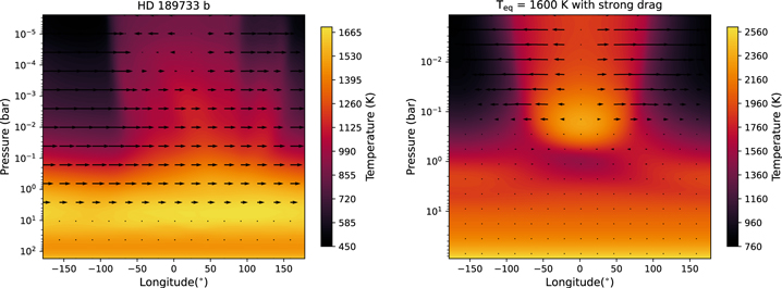

Figure 23. Refer to the following caption and surrounding text. — **Figure 23.** The temperatures (color scale) and winds (arrows) on the meridionally averaged equatorial plane of HD 189733 b (left) and those of our fiducial hot Jupiter atmosphere with strong drag from Tan & Komacek (2019; right). The substellar point is located at 0° longitude. A superrotating jet extends from approximately a few bar to 0.1 mbar level on HD 189733 b, whereas the strong-drag fiducial circulation is dominated by the day-to-night flow above 1 bar.
Download figure:
Standard image High-resolution image

Footnotes

11
Strictly speaking, it is the angular velocity held constant in a rotating 1D model. The top layer of the equivalent flow moves faster than the bottom one by H_atm ω, where H_atm is the atmospheric depth in the model and ω is the assumed rotational frequency applied to simulate the equatorial jet.
12
https://github.com/exoclime/VULCAN/blob/master/thermo/NCHO_photo_network.txt

Please wait… references are loading.