Abstract
Dark energy is believed to be responsible for the acceleration of the Universe. In this paper, we reconstruct the dark energy scalar field potential V(ϕ) using the Hubble parameter H(z) through Gaussian process analysis. Our goal is to investigate dark energy using various H(z) data sets and priors. We find that the selection of the prior and the H(z) data set significantly affects the reconstructed V(ϕ). We compare two models, Power Law and Free Field, to the reconstructed V(ϕ) by computing the reduced chi-square. The results suggest that the models are generally in agreement with the reconstructed potential within a 3σ confidence interval, except in the case of Observational H(z) data with the Planck 18 prior. Additionally, we simulate H(z) data to measure the effect of increasing the number of data points on the accuracy of reconstructed V(ϕ). We find that doubling the number of H(z) data points can improve the accuracy rate of reconstructed V(ϕ) by 5%–30%.
Original content from this work may be used under the terms of the Creative Commons Attribution 4.0 licence. Any further distribution of this work must maintain attribution to the author(s) and the title of the work, journal citation and DOI.
1. Introduction
In 1998, two independent teams, Riess et al. (1998) and Perlmutter et al. (1999), discovered that the expansion of the Universe is accelerating by observing the distant type Ia supernovae. Since then, cosmic acceleration has been accepted by cosmologists. Understanding the origin of acceleration is critical to understanding fundamental physics in the Universe. There are two explanations for the cosmic acceleration (Frieman et al. 2008). One is dark energy (Huterer & Shafer 2018), which is a new energy form with large negative pressure and repulsive gravity. The other is modified gravity (Ishak 2019), where general relativity breaks down on cosmological scales.
The simplest model for dark energy is vacuum energy, which mathematically corresponds to a cosmological constant that does not vary with space or time. In this model, dark energy is not a dynamic quantity. However, by introducing a new degree of freedom in the form of a scalar field ϕ, dark energy can become dynamical (Ratra & Peebles 1988; Wetterich 1988; Frieman et al. 1995; Zlatev et al. 1999). Recently, the results from DESI Collaboration et al. (2024) have motivated the search for dynamical dark energy models. The measurements of baryon acoustic oscillations (BAO) from DESI, when combined with either the cosmic microwave background (CMB) or type Ia supernovae individually, prefer ω0 > −1 and ωa < 0. There are also other dark energy models, including more complex scalar field models (Caldwell 2002; Carroll et al. 2003). In this article, we investigate the scalar field using observational H(z) data (OHD) (Yu et al. 2013) via the Gaussian process. OHD can be measured using different ways, such as cosmic chronometers (CC) and baryon acoustic oscillations (BAO). Unlike supernova observations, which measure H(z) indirectly through its integral along the line of sight, these methods can directly measure H(z) (Jesus et al. 2018).
Quintessence is a type of scalar field first introduced by Caldwell et al. (1998). According to this theory, quintessence represents a form of dark energy that changes over time. In order to study the properties of dark energy, it is useful to study the scalar field ϕ endowed with a dark energy scalar field potential V(ϕ). Recently, several works have focused on reconstructing the dark energy scalar field potential from cosmological data sets without making any assumptions about its form. For example, Jesus et al. (2022) used H(z) and Type Ia supernovae data to constrain the dark energy potential via the Gaussian process. They also compared the results obtained using different priors, namely Planck 18 and a large prior to assess the differences in the reconstruction. Elizalde et al. (2024) used 40 H(z) data points to reconstruct the dark energy potential through the Gaussian process in a model-independent manner. They compared the results obtained using two different kernel functions and three different H0 values.
To reconstruct the dark energy scalar field potential V(ϕ), we must choose priors and data sets. This paper aims to investigate how different priors and data sets affect the reconstruction results. We compare the reconstructed V(ϕ) using two priors: Planck 18 (P18) and Nine-Year Wilkinson Microwave Anisotropy Probe (WMAP9y). We also compare the reconstructed V(ϕ) using three data sets: CC, BAO, and OHD (a combination of CC and BAO). Through this comparison, we can determine the impact of using different individual data sets (CC and BAO) on the reconstructed V(ϕ). Additionally, we can compare the differences between the individual data sets (CC or BAO) and the combined data set (OHD) to understand the effect of combining different data sets on the reconstructed V(ϕ). With the advent of advancing technology, more H(z) data points are being released, which can potentially optimize V(ϕ). We compare two models, Power Law and Free Field, to the reconstructed V(ϕ) by computing the reduced chi-square. This paper will also explore the impact of additional data points on the reconstruction results. The following paper will discuss these topics.
This work is structured as follows: In Section 2, we derive the function of the dark energy scalar field potential V(ϕ). Section 3 compiles the CC data set, BAO data set, and priors in Tables 1, 2, and 3, respectively. In Section 4, we reconstruct V(ϕ) using the CC, BAO, and OHD data sets via the Gaussian process. Two models, Power Law and Free Field, are compared to the reconstructed V(ϕ) by computing the reduced chi-square. We also simulate H(z) to investigate how the accuracy of V(ϕ) reconstruction improves as we increase the number of H(z) data points. Finally, Section 5 provides the conclusion and discussion of this paper.
Table 1. Compiled CC Data
| Redshift z | H(z) a ±1σ Error | References |
|---|---|---|
| 0.07 | 69 ± 19.6 | Zhang et al. (2014) |
| 0.1 | 69 ± 12 | Stern et al. (2010) |
| 0.12 | 68.6 ± 26.2 | Zhang et al. (2014) |
| 0.17 | 83 ± 8 | Stern et al. (2010) |
| 0.1791 | 75 ± 4 | Moresco et al. (2012) |
| 0.1993 | 75 ± 5 | Moresco et al. (2012) |
| 0.2 | 72.9 ± 29.6 | Zhang et al. (2014) |
| 0.27 | 77 ± 14 | Stern et al. (2010) |
| 0.28 | 88.8 ± 36.6 | Zhang et al. (2014) |
| 0.3519 | 83 ± 14 | Moresco et al. (2012) |
| 0.382 | 83 ± 13.5 | Moresco et al. (2016) |
| 0.4 | 95 ± 17 | Stern et al. (2010) |
| 0.4004 | 77 ± 10.2 | Moresco et al. (2016) |
| 0.4247 | 87.1 ± 11.2 | Moresco et al. (2016) |
| 0.4497 | 92.8 ± 12.9 | Moresco et al. (2016) |
| 0.47 | 89 ± 49.6 | Ratsimbazafy et al. (2017) |
| 0.4783 | 80.9 ± 9 | Moresco et al. (2016) |
| 0.48 | 97 ± 62 | Stern et al. (2010) |
| 0.5929 | 104 ± 13 | Moresco et al. (2012) |
| 0.6797 | 92 ± 8 | Moresco et al. (2012) |
| 0.7812 | 105 ± 12 | Moresco et al. (2012) |
| 0.8 | 113.1 ± 25.22 | Jiao et al. (2023) |
| 0.8754 | 125 ± 17 | Moresco et al. (2012) |
| 0.88 | 90 ± 40 | Stern et al. (2010) |
| 0.9 | 117 ± 23 | Stern et al. (2010) |
| 1.037 | 154 ± 20 | Moresco et al. (2012) |
| 1.3 | 168 ± 17 | Stern et al. (2010) |
| 1.363 | 160 ± 33.6 | Moresco (2015) |
| 1.43 | 177 ± 18 | Stern et al. (2010) |
| 1.53 | 140 ± 14 | Stern et al. (2010) |
| 1.75 | 202 ± 40 | Stern et al. (2010) |
| 1.965 | 186.5 ± 50.4 | Moresco (2015) |
Note.
a H(z) figures are in the unit of kms−1 Mpc−1.Download table as: ASCIITypeset image
Table 2. Compiled BAO Data
| Redshift z | H(z) ± 1σ Error | References |
|---|---|---|
| 0.24 | 82.37 ± 3.94 | Gaztañaga et al. (2009) |
| 0.3 | 78.83 ± 6.58 | Oka et al. (2014) |
| 0.31 | 78.39 ± 5.46 | Wang et al. (2017) |
| 0.35 | 88.1 ± 9.45 | Chuang & Wang (2013) |
| 0.36 | 80.16 ± 4.37 | Wang et al. (2017) |
| 0.38 | 81.74 ± 3.4 | Alam et al. (2017) |
| 0.43 | 89.36 ± 4.89 | Gaztañaga et al. (2009) |
| 0.44 | 85.48 ± 8.59 | Blake et al. (2012) |
| 0.51 | 90.67 ± 3.66 | Alam et al. (2017) |
| 0.52 | 94.61 ± 4.2 | Wang et al. (2017) |
| 0.56 | 93.59 ± 3.96 | Wang et al. (2017) |
| 0.57 | 96.59 ± 8.76 | Anderson et al. (2014) |
| 0.59 | 98.75 ± 4.66 | Wang et al. (2017) |
| 0.6 | 90.96 ± 7.04 | Blake et al. (2012) |
| 0.61 | 97.59 ± 3.97 | Alam et al. (2017) |
| 0.64 | 99.09 ± 4.53 | Wang et al. (2017) |
| 0.73 | 100.69 ± 8.03 | Blake et al. (2012) |
| 2.33 | 223.99 ± 11.12 | Bautista et al. (2017) |
| 2.34 | 222.105 ± 10.38 | Delubac et al. (2015) |
| 2.36 | 226.24 ± 11.18 | Font-Ribera et al. (2014) |
Download table as: ASCIITypeset image
Table 3. Compiled Priors
| Prior | H0 | Ωk0 | ΩM0 | References |
|---|---|---|---|---|
| P18 | 67.4 ± 0.5 | 0.001 ± 0.002 | 0.315 ± 0.007 | Planck Collaboration et al. (2020) |
| WMAP9y | 70.0 ± 2.2 | −0.037 ± 0.043 | 0.279 ± 0.025 | Bennett et al. (2013) |
Download table as: ASCIITypeset image
2. Theory
Quintessence is a model of dark energy characterized by a time-dependent scalar field. The properties of quintessence are represented by the dark energy scalar field potential V(ϕ). In order to reconstruct V(ϕ) with H(z) data sets, it is necessary to derive the equation for V(ϕ). This can be done in two steps: first, by deriving the energy density ρϕ and pressure Pϕ of the scalar field, and second, by deriving V(ϕ).
2.1. Energy Density ρϕ and Pressure Pϕ
The energy-momentum tensor for the scalar field  is
is
where V(ϕ) represents the dark energy scalar field potential. In this paper, we assume that the field is mostly homogeneous, and thus the energy momentum for the zero-order part of it, ϕ(0)(t), is
Using Equation (2), we can obtain the energy density ρϕ
and the pressure Pϕ
. The energy density is given by the time–time component,  . For the homogeneous field, the pressure Pϕ
is equal to
. For the homogeneous field, the pressure Pϕ
is equal to  , so
, so


2.2. Dark Energy Scalar Field Potential V(z)
Within the framework of general relativity, the evolution of the Universe is described by the Friedmann equation and the acceleration equation. In our derivation, we use natural units. At late times in the universe, the radiation density is much smaller than other types of densities. Therefore, we can neglect the radiation density in the Friedmann equation, which is given by

where ρmat is the matter density in the universe, k represents the curvature of the universe, and a is the scalar factor. The acceleration equation is

By substituting ρϕ and Pϕ from Equations (3) and (4) into Equations (5) and (6), we obtain


To obtain the dark energy scalar field potential V(z), we need to eliminate the  term in the equation. Note that
  . Multiplying Equation (7) by 2 and adding it to Equation (8) gives us

In order to reconstruct the scalar field potential of dark energy in the redshift space, we need to convert V(ϕ) to V(z). As we have assumed a homogeneous universe in this paper, the scalar field ϕ only varies with time t. The relationship between time and redshift is given by

where z represents the redshift and a(t0) and a(t1) represent the scale factor at the present time and some past time, respectively. According to Equation (10), time can be expressed as a function of redshift, i.e., t = t(z), we can invert V(ϕ(t)) to V(ϕ(z)) and then to V(z). Equation (9) can be rewritten as
According to Equation (11), in order to determine the values of V(z) and σV (z), it is necessary to know the values of H, d H/d z, H0, Ωk0, and ΩM0 along with their 1σ uncertainties (68% confidence regions). We use the H(z) data set via the Gaussian process to obtain H and d H/d z in the range of z ∈ [0, 2.5], while H0, Ωk0, and ΩM0 are chosen as priors. This paper uses the 1σ uncertainty of V(z), which is obtained by propagating the uncertainties. For a function f = f(x1, x2,…,xn ), the variance formula of f is given by

Where σi represents the standard deviation of xi , while σij denotes the covariance between xi and xj . It is defined as:

xik represents the kth value of xi , and the total number of xi is denoted as N.
According to Equation (12), the error equation for V(z) is
Here,  represents d
H/d
z. σH
, σH0,
represents d
H/d
z. σH
, σH0,  ,
,  , and
, and  represent the 1σ uncertainty of H, H0,
  , Ωk0, and ΩM0, respectively.
  represents the covariance between H and
  .
.
3. Data and Priors
The H(z) data set in Equation (11) can be obtained from OHD. OHD comprises measurements of the Hubble parameter H(z) at different redshifts, using various cosmological probes such as CC and BAO. In this paper, the CC and BAO data sets are used to reconstruct H(z) via the Gaussian process. CC provides a model-independent way to obtain H(z) data directly calculated from the differential ages of galaxies

BAO can be measured from the correlation function (Wang et al. 2017) or power spectrum (Anderson et al. 2012) of the galaxy distribution. The Hubble parameter H(z), detectable in the direction of the BAO’s line of sight, can be parameterized as

The CC and BAO data used in this paper are compiled in Tables 1 and 2, respectively. We reconstruct V(z) in Equation (12) using the CC, BAO, and OHD (CC+BAO) data sets. We compare the influence of different individual data sets (CC and BAO) on the reconstructed V(z). Additionally, we compare the impact of using individual data sets (CC or BAO) versus the combined data set (OHD) on the reconstructed V(z).
The OHD data points are collected from different galaxies using various methods. We assume that data points obtained through different methods are independent, with no covariance between them. Within the OHD data set, there are 15 data points proposed by Moresco et al. (2012), Moresco (2015), and Moresco et al. (2016), all obtained through the same method. The researchers responsible for these data points have introduced a method known as the Cosmic chronometers covariance (Moresco et al. 2020) 5 to estimate the covariance between them. We take this covariance matrix into account when reconstructing the dark energy scalar field potential in Section 4.1.
According to Equations (11) and (14), it is necessary to have priors on H0, Ωk0, and ΩM0 in order to reconstruct the Hubble parameter H(z). To compare the effects of different priors on the results, we choose two different priors, P18 and WMAP9y, to reconstruct H(z). The priors are compiled in Table 3. We choose two priors and three data sets for the reconstruction of V(z), resulting in six different combinations of data set_prior. These reconstructed results are shown in Figures 1, 2, 3, 4, 5, 6.
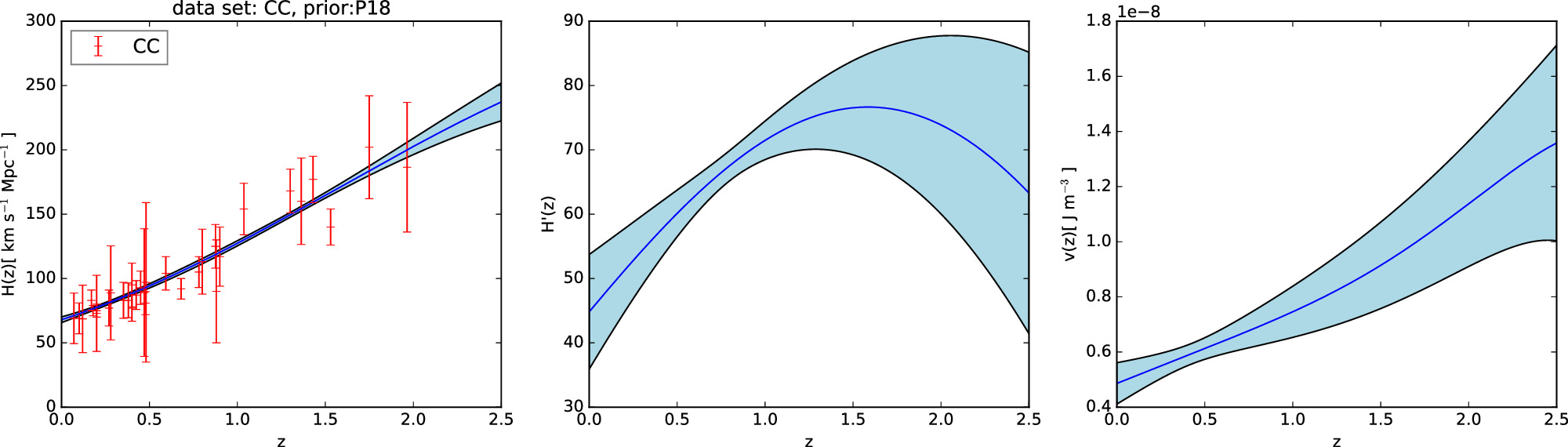
Figure 1. Gaussian process reconstruction of H(z) (left) from CC data set,  (middle), and V(z) (right) with P18 prior. The blue-shaded region is the 1σ uncertainty of the reconstruction.
Download figure:
Standard image High-resolution image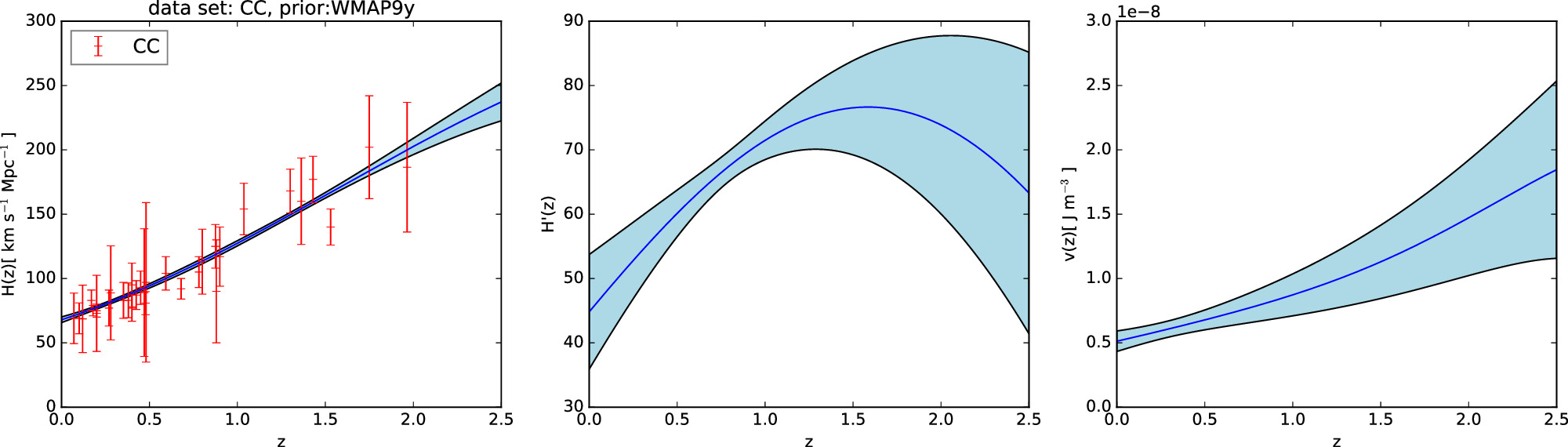
Figure 2. Gaussian process reconstruction of H(z) (left) from CC data set,  (middle), and V(z) (right) with WMAP9y prior. The blue-shaded region is the 1σ uncertainty of the reconstruction.
Download figure:
Standard image High-resolution image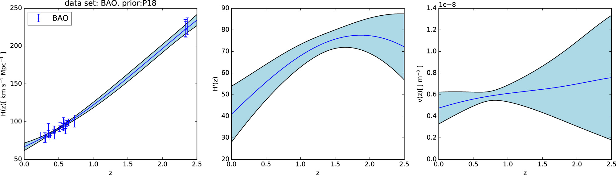
Figure 3. Gaussian process reconstruction of H(z) (left) from BAO data set,  (middle), and V(z) (right) with P18 prior. The blue-shaded region is the 1σ uncertainty of the reconstruction.
Download figure:
Standard image High-resolution image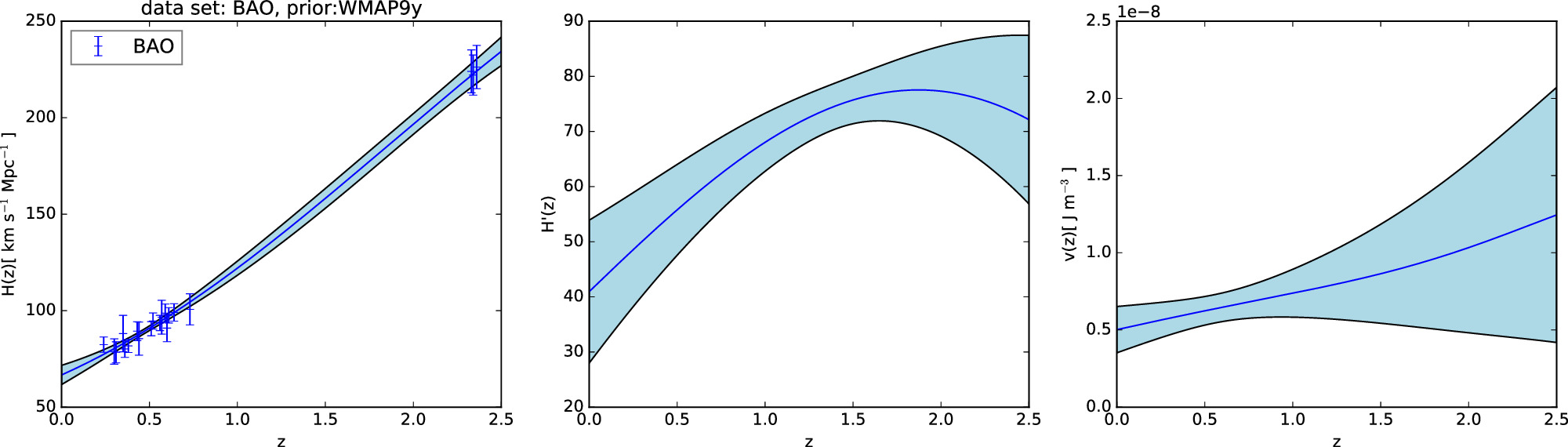
Figure 4. Gaussian process reconstruction of H(z) (left) from BAO data set,  (middle), and V(z) (right) with WMAP9y prior. The blue-shaded region is the 1σ uncertainty of the reconstruction.
Download figure:
Standard image High-resolution image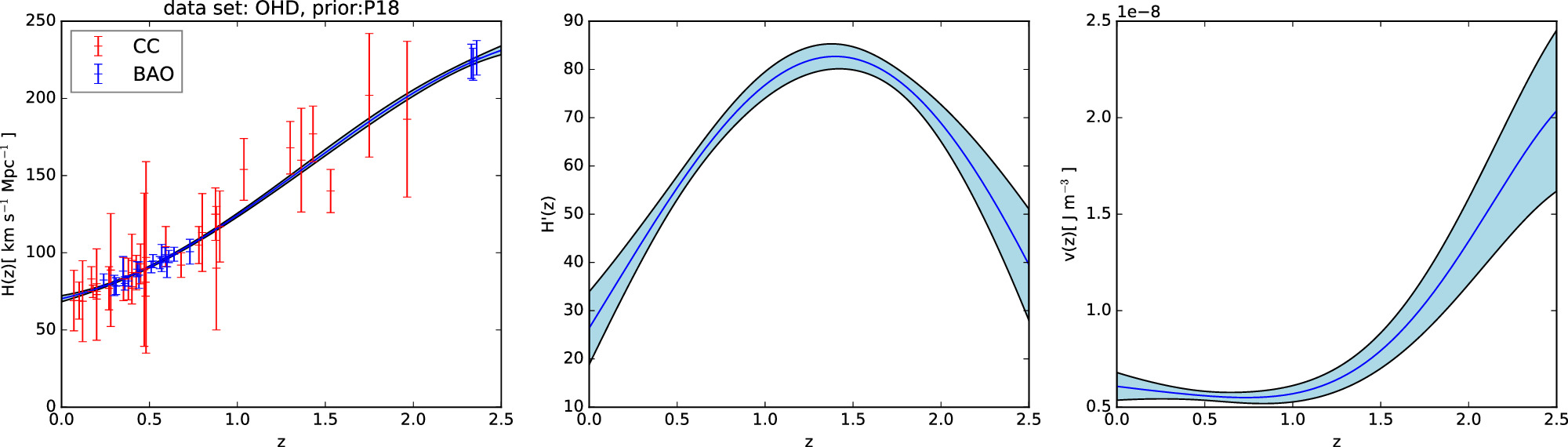
Figure 5. Gaussian process reconstruction of H(z) (left) from OHD data set,  (middle), and V(z) (right) with P18 prior. The OHD data set contains CC data points in red and BAO data points in blue. The blue-shaded region is the 1σ uncertainty of the reconstruction.
Download figure:
Standard image High-resolution image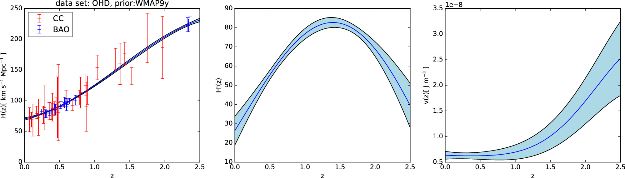
Figure 6. Gaussian process reconstruction of H(z) (left) from OHD data set,  (middle), and V(z) (right) with WMAP9y prior. The OHD data set contains CC data points in red and BAO data points in blue. The blue-shaded region is the 1σ uncertainty of the reconstruction.
Download figure:
Standard image High-resolution image4. Reconstruction of the Dark Energy Scalar Field Potential
4.1. Reconstruction
The Gaussian process is a popular method for reconstructing a function without assuming any parameters in the function (Yahya et al. 2014; Cai et al. 2016; Sun et al. 2021). The Gaussian process can describe the observational data by a distribution function f(z) with mean value and error at each point z. The reconstructed functions at different points z and  are correlated by a covariance function
  . There are many covariance functions available (Rasmussen & Williams 2006; Seikel & Clarkson 2013). In this paper, we use the Squared Exponential covariance function, which is widely used in the reconstruction of H(z) by the Gaussian process (Seikel et al. 2012; Busti et al. 2014; Sun et al. 2021). The Squared Exponential covariance function is given by

This function depends on two hyperparameters: σf
and l. These hyperparameters determine the amplitude and the coherence length of the function, respectively. In this paper, the Gaussian process is used to reconstruct the H(z) function from the data points listed in Tables 1 and 2. Compared to other reconstruction methods like Artificial Neural Networks (ANN), the distribution function is a Gaussian distribution, allowing it to be differential at any point z. This property can be utilized to easily reconstruct the first derivative of the Hubble parameter H(z) with respect to z, denoted as  . The code used in this paper is Gaussian processes in Python (GAPP) proposed by Seikel et al. (2012).
To reconstruct the dark energy scalar field potential V(z), we need the reconstructed H(z) and  values with 1σ uncertainty. Additionally, we require the a priors of H0, Ωk0, and ΩM0 as listed in Table 3, along with the covariance
  between H(z) and
  in Equation (14). The use of the Gaussian process enables us to reconstruct H(z) and
  from the observational data. To determine the impact of different data sets and priors on V(z), we consider three data sets (CC, BAO, and OHD), and two different priors (P18 and WMAP9y). This results in six different reconstructed V(z) outcomes: CC+P18 as shown in Figure 1, CC+WMAP9y as shown in Figure 2, BAO+P18 as shown in Figure 3, BAO+WMAP9y as shown in Figure 4, OHD+P18 as shown in Figure 5, and OHD+WMAP9y as shown in Figure 6.
The reconstructed V(z) can validate and compare various models of the dark energy scalar field. In this study, we have selected two specific models (Jesus et al. 2022): the Free Field (FF) model (Ratra 1991; Ureña-López & Reyes-Ibarra 2009) and the Power Law (PL) (Peebles & Ratra 1988; Ratra & Peebles 1988) model:

where  .
.


The comparison between the reconstructed V(z) and these models is illustrated in Figure 7.
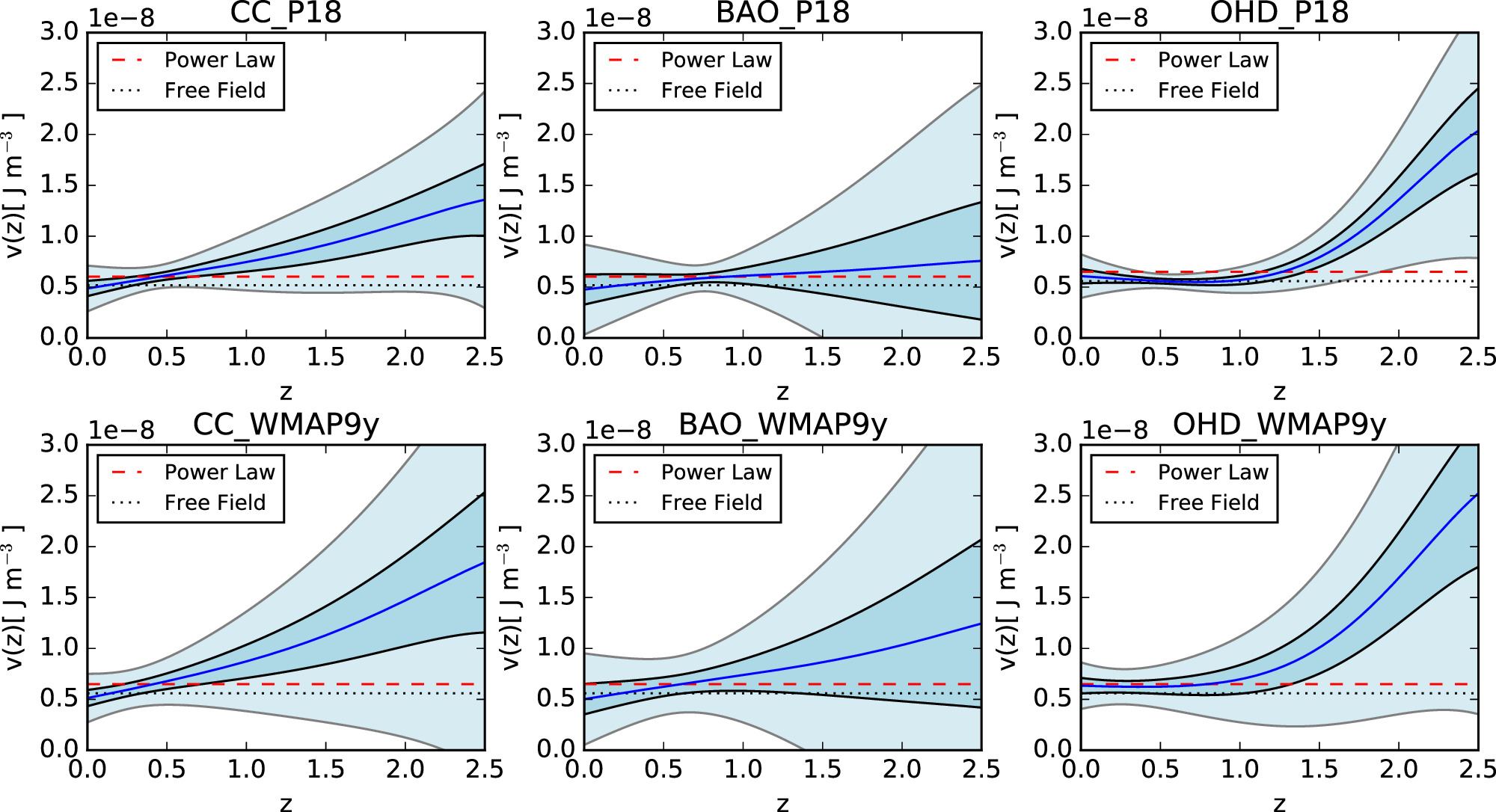
Figure 7. Gaussian process reconstruction of V(z) from six different data sets and priors: CC with prior P18 (upper left), BAO with prior P18 (upper center), OHD with prior P18 (upper right), CC with prior WMAP9y (bottom left), BAO with prior WMAP9y (bottom center), and OHD with prior WMAP9y (bottom right). The shaded blue regions represent the 1σ and 3σ uncertainty of the reconstruction. The red dashed line and the black dotted line represent the dark energy scalar field models Power Law and Free Field, respectively.
Download figure:
Standard image High-resolution imageAs depicted in Figure 7, the Power Law and Free Field models fall within the 3σ range of reconstructed V(z) for five data set_prior conditions (CC_P18, CC_WMAP9y, BAO_P18, BAO_WMAP9y, and OHD_WMAP9y) in this paper. However, for the data set: OHD, prior: P18 condition, at high redshift (z ≳ 1.5), these models fall outside the 3σ range of the reconstructed V(z). This implies that the Power Law model and Free Field model are excluded at high redshift in the data set: OHD, prior: P18 condition. Based on the figure, at low redshift (z ≲ 0.5 for CC_P18 and CC_WMAP9y; z ≲ 1 for OHD_WMAP9y), both models exhibit a high level of compatibility, falling within a deviation of less than 1σ from the reconstructed V(z). For the remaining redshift range, compatibility is within 3σ. These models fit the reconstructed V(z) better at low redshifts. Meanwhile, for BAO_P18 and BAO_WMAP9y conditions across the entire redshift range from 0 to 2.5, both models are almost within 1σ of the reconstructed V(z), indicating a high level of compatibility with the reconstructed V(z) under these conditions.
To assess which model provides a better fit to the reconstructed V(z) across different data sets and priors depicted in Figure 7, we computed the reduced chi-square ( ) values between the reconstructed V(z) and various models. The formula of
  is:
is:
where N represents the number of data points, and p represents the number of parameters in the model. Vm
represents the V(z) provided by the theoretical model. Vr
and  denote the reconstructed V(z) and its 1σ uncertainty, respectively. We computed the
  between the reconstructed V(z) and the theoretical model’s V(z), where the z-values are the observed z-values as presented in Tables 1 and 2. Consequently, N equals 32 for CC_P18 and CC_WMAP9y, 20 for BAO_P18 and BAO_WMAP9y, and 52 for OHD_WMAP9y. The result of
  is compiled in Table 4.
Table 4.
 Comparison: Reconstructed V(z) vs. Different Models
| data set_prior | Model |

|
|---|---|---|
| CC_P18 | Power Law | 4.92 |
| Free Field | 8.13 | |
| CC_WMAP9y | Power Law | 12.18 |
| Free Field | 17.59 | |
| BAO_P18 | Power Law | 0.24 |
| Free Field | 0.41 | |
| BAO_WMAP9y | Power Law | 2.26 |
| Free Field | 3.33 | |
| OHD_WMAP9y | Power Law | 34.97 |
| Free Field | 41.40 | |
Download table as: ASCIITypeset image
In the first column of Table 4, data set_prior indicates the data set and prior used for reconstructing V(z). Table 4 reveals that across all data set_priors (CC_P18, CC_WMAP9y, BAO_P18, BAO_WMAP9y, OHD_WMAP9y), the Power Law model consistently has lower  values compared to the Free Field model. This suggests that, in general, the Power Law model provides a better fit to the reconstructed V(z) data. For both the Power Law model and the Free Field model, the BAO_P18 data set_prior consistently results in lower
  values compared to other data set_prior conditions. This indicates that the BAO_P18 data set_prior is a better fit for both models when considering the
  values alone. For the CC and BAO data sets, the choice of prior (P18 versus WMAP9y) significantly affects the fit quality, with P18 generally providing better results.
4.2. Comparison
In this paper, we aim to compare the effects of different priors and data sets on the reconstructed V(z). We divide the six V(z) results mentioned in Section 4.1 into two categories. The first category is the comparison of the same data set with different priors, as shown in Figure 8. We observe that the choice of priors has a substantial effect on the reconstructed V(z), and it is worth noting that the P18 prior consistently results in narrower uncertainty regions across all data sets, indicating more precise reconstructions compared to the WMAP9y prior. The second category is the comparison of the same prior with different data sets: CC, BAO, and OHD (which combines the CC and BAO data sets), as shown in Figure 9. We observe a significant difference in the reconstructed V(z) based on different data sets. Different data sets lead to distinct trends in the reconstructed V(z). The CC data set consistently exhibits a narrow uncertainty band, indicating higher precision compared to the BAO data set. CC results are consistent with BAO within 1.19σ for P18 prior (left panel of Figure 9) and 0.62σ for WMAP9y prior (right panel of Figure 9), justifying their combination to derive results for the OHD data set. The combined OHD data set shows a trend distinct from CC and BAO, highlighting the impact of combining data sets. These results indicate that obtaining more accurate H(z) data points and precise priors will enhance the accuracy and reliability of the reconstructed V(z).
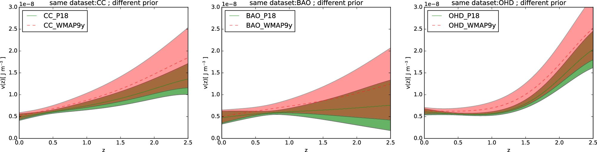
Figure 8. Comparison of the reconstructed V(z) from the CC (left), BAO (center), and OHD (right) data sets using different priors. The solid green line represents the mean of V(z) with P18 prior, while the dashed red line represents the mean of V(z) with WMAP9y prior. The green and red shaded regions correspond to the 1σ uncertainty of V(z) with P18 and WMAP9y, respectively.
Download figure:
Standard image High-resolution image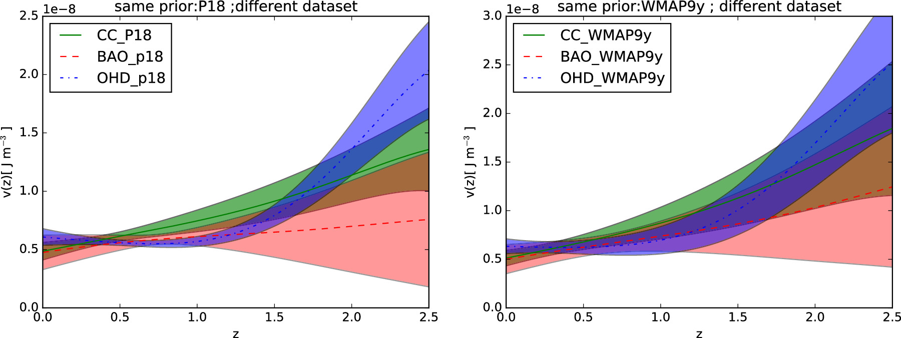
Figure 9. Comparison of the reconstructed V(z) using the same prior, P18 (left) and WMAP9y (right), from the different data sets. The solid green line represents the mean V(z) reconstructed from the CC data set, the dashed red line represents the mean V(z) reconstructed from the BAO data set, and the dashed–dotted blue line represents the mean V(z) reconstructed from the OHD data set. The green, red, and blue-shaded regions represent the 1σ uncertainty of V(z) from the CC, BAO, and OHD data sets, respectively.
Download figure:
Standard image High-resolution image4.3. Simulation
To quantify the influence of the reconstructed V(z) results based on the number of H(z) data points, we simulate additional H(z) data points using the available H(z) data sets in Tables 1 and 2. The simulation is based on the principle of generating Hsim(z) data points that are similar to the available data sets. The simulation of Hsim(z) consists of two main steps. In the first step, we simulate Hm (z), which represents the mean value of the simulated Hubble parameter Hsim(z) at different redshifts z. In the second step, we generate the uncertainty of the Hubble parameter, σH (z). The Hsim(z) at redshift zsim is

To quantify the improvement of the V(z) result by increasing the number of H(z) data points, we doubled the number of H(z) data points, which required simulating 32 CC and 20 BAO data points similar to the data sets compiled in Tables 1 and 2. In this paper, we simulate redshift zsim with the same density distribution as the observational data sets. This approach is more reasonable than a uniform distribution, considering the current technology and available data sets.
In the first step, we reconstruct the distribution of  using the Gaussian process with the observational data sets. The Gaussian process reconstructs the distribution of H(z), and we generate
  using the Gaussian distribution
  .
.  is the mean of the distribution represented by the black points in the blue line in the left panel of Figure 10, and
  is shown in the left panel of Figure 10 with error bars within the 95% confidence interval. We select
  within this interval. The simulated
  is shown in the right panel of Figure 10.
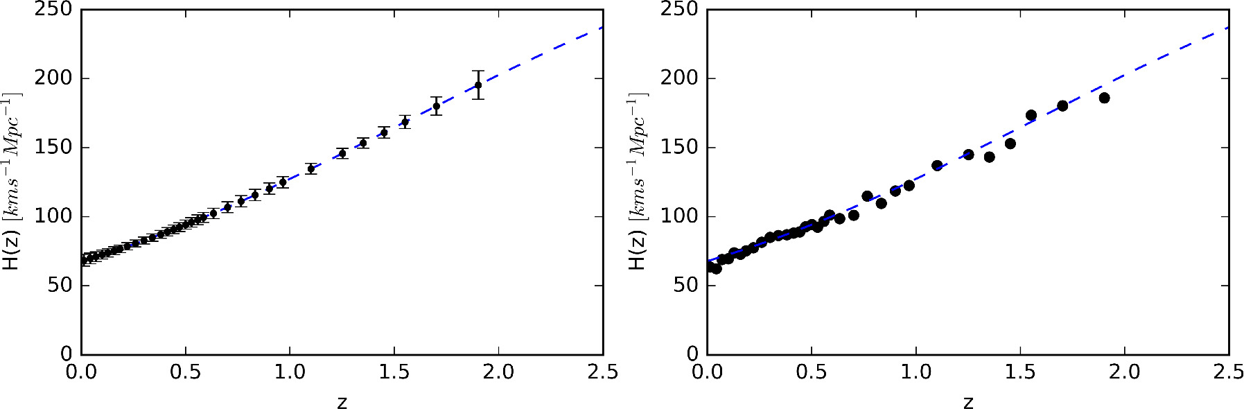
Figure 10. Left: the reconstructed Hubble parameter at redshift zsim with 2σ error bars. Right: simulated  in Equation (22). The blue dashed line represents the mean value of the reconstructed H(z).
Download figure:
Standard image High-resolution imageIn step two, we employ the method proposed by Ma & Zhang (2011) to generate the uncertainty  . To assess the uncertainty of the H(z) data sets, we plot the z−σH
in Figure 11. In the figure, we exclude the outliers in the blue circle and bound the remaining data points with two straight lines: σ+ = 8.2z + 34.3 in red and σ− = 7.4z + 2.7 in green. The uncertainty of H at the z point is estimated by a Gaussian distribution N(σ0(z),
. To assess the uncertainty of the H(z) data sets, we plot the z−σH
in Figure 11. In the figure, we exclude the outliers in the blue circle and bound the remaining data points with two straight lines: σ+ = 8.2z + 34.3 in red and σ− = 7.4z + 2.7 in green. The uncertainty of H at the z point is estimated by a Gaussian distribution N(σ0(z), (z)), where the mean is the midpoint of the lines σ0 = 7.8z + 18.5 and
(z) = (σ+ − σ−)/4. We choose
(z) such that the generated σ falls within 95% of the Gaussian distribution. Using Equation (22), we obtain the simulated Hubble parameter
 , as shown in Figure 12.
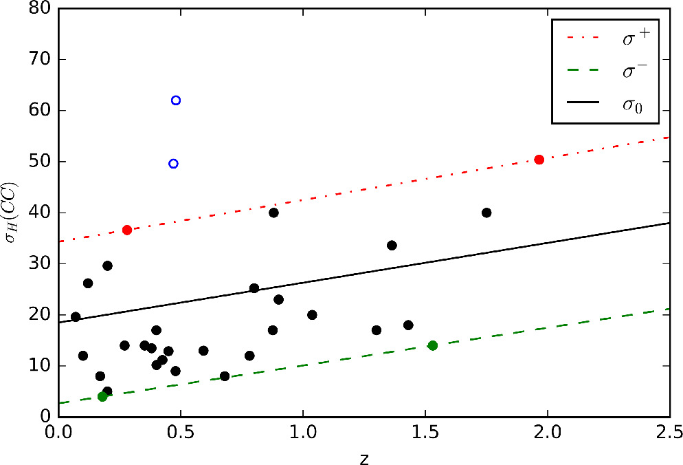
Figure 11. 1σ uncertainty of H(z) in the CC data set. The solid dots and blue circles represent non-outliers and outliers, respectively. The red dashed–dotted line represents the upper bound of the data points’ uncertainty, denoted as σ+, while the green dashed line represents the lower bound of the uncertainty, denoted as σ−. The solid black line represents the mean uncertainty σ0.
Download figure:
Standard image High-resolution image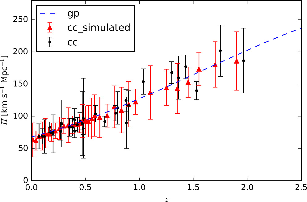
Figure 12. Simulated  data set based on CC data set using our method. The CC data set is also shown for comparison. The blue dashed line denotes the mean value of reconstructed H(z) from the CC data set.
Download figure:
Standard image High-resolution imageUsing the reconstructed method described in Section 4.1 with the CC and simulated CC data points, we can reconstruct the dark energy scalar field potential V(z) for the P18 prior and WMAP9y prior. Similarly, we can reconstruct V(z) for the same priors using BAO and simulated BAO data points, as well as using OHD and simulated OHD data points. The improvement in accuracy of V(z) can be quantified by

where σ(z) is the error in the reconstructed dark energy scalar field potential V(z) using the observed Hubble parameter at redshift z, and  is the error in V(z) reconstructed using both the observed and simulated H(z) at redshift z. The improvement rate varies depending on the simulated H(z) used, with a range of approximately 5% to 30%. Thus, doubling the number of Hubble parameter H(z) results in an increase in the accuracy of the dark energy scalar field potential by 5%–30%.
5. Discussions and Conclusions
In this paper, we reconstruct the dark energy scalar field potential V(ϕ) using the Gaussian process. Jesus et al. (2022) and Elizalde et al. (2024) also reconstructed the dark energy scalar field potential using the Gaussian process. The details of the reconstructions are different from each other. To reconstruct the scalar field potential, we need both the data set and prior, as well as a choice of covariance function for the Gaussian process. We use the updated CC, BAO, and OHD (CC+BAO) data sets and analyze the influence of different data sets on the reconstructed scalar field potential. In contrast, Jesus et al. (2022) used the CC and SN1a data sets, while Elizalde et al. (2024) used only the OHD data set. Regarding priors, we chose P18 and WMAP9y to analyze their influence on the reconstructed scalar field potential, while Jesus et al. (2022) used P18 and a large prior, and Elizalde et al. (2024) used three different priors. For the covariance function, both we and Jesus et al. (2022) chose the Squared Exponential function, whereas Elizalde et al. (2024) chose two different covariance functions: the Squared Exponential and the Matern (v = 9/2) covariance functions. Based on the  values computed between the reconstructed V(z) and the models chosen in Section 4.1, we find that the Power Law model tends to perform better overall than the Free Field model. Additionally, V(z) reconstructed using BAO_P18 data set_prior demonstrates a better fit to the models compared to CC_P18, CC_WMAP9y, BAO_WMAP9y, and OHD_WMAP9y. Notably, in the case of OHD_P18, the models are excluded at a significance level of 3σ in the high-redshift region (z ≳ 1.5). Our results show that both different data sets and different priors have a significant impact on the reconstructed V(ϕ). The study of dark energy is crucial to understanding the acceleration of the Universe. A scalar field is a viable solution to explain dark energy, and the dark energy scalar field potential V(ϕ) provides an effective approach to studying it. In this paper, we update the available CC and BAO data sets and provide detailed procedures to reconstruct V(ϕ) via the Gaussian process. While previous studies have also used the Gaussian process to reconstruct V(ϕ) (Jesus et al. 2022; Elizalde et al. 2024), our study is the first to compare the impact of different data sets and priors on the reconstructed V(ϕ).
In Section 2.2, we present a step-by-step derivation of the dark energy scalar field potential V(ϕ) and its 1σ uncertainty σV
. Then we show the reconstructed V(ϕ) using CC, BAO, or OHD data sets with either the P18 or WMAP9y priors in Figures 1, 2, 3, 4, 5, and 6. In the future, as more data points become available and more accurate priors for H0, ΩM0, and Ωk0 are obtained, we can enhance the accuracy and reliability of our V(z) reconstructions. These improvements will allow us to rigorously validate the V(z) models. In the following phase of our work, we will validate existing models by comparing them with the reconstructed V(z) data. Furthermore, we will explore the potential for proposing new models that are consistent with our reconstructed V(z). To assess the impact of different data sets and priors on the reconstructed V(ϕ), we compare the results. Our analysis reveals that both different data sets and different priors have a great influence on the reconstructed V(ϕ), as shown in Figures 8 and 9. Especially in Figure 9, we compare the impact on the reconstructed V(z) using three different data sets: CC, BAO, and OHD (CC+BAO). This allows us to observe the influence of different individual data sets (CC versus BAO) and also compare the individual data sets (CC or BAO) with the combined data set (OHD). In order to measure the improvement in accuracy of V(ϕ) resulting from an increased number of H(z) data points, we conduct a simulation of H(z) data. The simulation process consists of two parts:  , where Hm
(z) is the mean value of the simulated Hsim(z) and
, where Hm
(z) is the mean value of the simulated Hsim(z) and  is the error of the simulated Hsim(z). We simulate
  to match the density of observed H(z) data points. By doubling the number of H(z) data points, we find that the accuracy of reconstructed V(ϕ) increased by around 5%–30%.
The accuracy of the reconstructed V(ϕ) is significantly affected by the simulation of H(z). In this study, we simulate H(z) using the Gaussian process based on the observed Hubble parameter H(z). The simulated H(z) varies each time, and the different results of the simulation have a considerable impact on the reconstructed V(ϕ). The improvement in accuracy rate can vary from 5% to 30% due to the different simulated H(z). As discussed in Section 4.3, the number of data points is important. Therefore, in the future, we will focus on obtaining more H(z) data to enhance the accuracy of the dark energy scalar field potential V(ϕ).
Acknowledgments
We thank Jie-Feng Chen and Yu-Chen Wang for their useful discussions. This work was supported by the National SKA Program of China (2022SKA0110202) and the National Science Foundation of China (grants No. 11929301).
Software: Gaussian processes in Python (Seikel et al. 2012).