The following article is Free article

CONSTRAINING THE EPOCH OF REIONIZATION FROM THE OBSERVED PROPERTIES OF THE HIGH-z UNIVERSE

Eduard Salvador-Solé, Alberto Manrique, Rafael Guzman, José Miguel Rodríguez Espinosa, Jesús Gallego, Artemio Herrero, J. Miguel Mas-Hesse, and Antonio Marín Franch

Published 2016 December 29 • © 2016. The American Astronomical Society. All rights reserved.
The Astrophysical Journal, Volume 834, Number 1Citation Eduard Salvador-Solé et al 2017 ApJ 834 49DOI 10.3847/1538-4357/834/1/49

Download Article PDF

DownloadArticle ePub

You need an eReader or compatible software to experience the benefits of the ePub3 file format.

Article metrics

1142 Total downloads
0 Video abstract views

Permissions

Get permission to re-use this article

Dates

Received 2016 March 23
Revised 2016 October 14
Accepted 2016 November 5
Published 2016 December 29

Keywords

cosmology: dark ages, reionization, first stars; evolution; galaxies: formation; quasars: supermassive black holes; stars: Population III

Journal RSS

Create or edit your corridor alerts

What are corridors?

ABSTRACT

We combine observational data on a dozen independent cosmic properties at high-z with the information on reionization drawn from the spectra of distant luminous sources and the cosmic microwave background (CMB) to constrain the interconnected evolution of galaxies and the intergalactic medium since the dark ages. The only acceptable solutions are concentrated in two narrow sets. In one of them reionization proceeds in two phases: a first one driven by Population III stars, completed at $z\sim 10$ , and after a short recombination period a second one driven by normal galaxies, completed at $z\sim 6$ . In the other set both kinds of sources work in parallel until full reionization at $z\sim 6$ . The best solution with double reionization gives excellent fits to all the observed cosmic histories, but the CMB optical depth is 3σ larger than the recent estimate from the Planck data. Alternatively, the best solution with single reionization gives less good fits to the observed star formation rate density and cold gas mass density histories, but the CMB optical depth is consistent with that estimate. We make several predictions, testable with future observations, that should discriminate between the two reionization scenarios. As a byproduct our models provide a natural explanation to some characteristic features of the cosmic properties at high-z, as well as to the origin of globular clusters.

Export citation and abstractBibTeX RIS

Previous article in issue

Next article in issue

1. INTRODUCTION

Reionization of the cosmic gas after it became essentially neutral at a redshift $z\sim 1100$ plays a crucial role in the galaxy formation process. Unfortunately, the details of the epoch of reionization (EoR) are to a large extent unknown.

The absence of global absorption shortward of the rest-frame Lyman-α (Lyα) line in the spectra of quasars at $z\lt 3$ made Gunn & Peterson (1965) realize that the hydrogen present in the nearby intergalactic medium (IGM) was ionized ( ${\bar{x}}_{{\rm{H}}{\rm{I}}}\lesssim {10}^{-4}$ ) except for small intervening systems yielding discrete absorption lines, the so-called Lyα forest. The Gunn–Peterson trough caused by neutral intergalactic hydrogen was finally found by Becker et al. (2001) and Djorgovski et al. (2001) in the spectra of quasars at $z\sim 6$ , suggesting the value for redshift ${z}_{\mathrm{ion},{\rm{H}}}$ of full hydrogen ionization.

Several subsequent studies using (a) the mean opacity of the Lyα forest (Fan et al. 2006); (b) the size of the proximity zone around quasars (Wyithe et al. 2005; Fan et al. 2006; Bolton & Haehnelt 2007a; Lidz et al. 2007; Maselli et al. 2007); (c) the detection of damping wing absorption by neutral IGM in quasar spectra (Mesinger & Haiman 2004, 2007; Mortlock et al. 2011b); (d) its non-detection in the spectra of gamma-ray bursts (Totani et al. 2006; McQuinn et al. 2007); (e) the abundance of Lyα emitters (LAEs; Malhotra & Rhoads 2004; Haiman & Cen 2005; Furlanetto et al. 2006; McQuinn et al. 2007; Mesinger & Furlanetto 2008; Ouchi et al. 2010; Jensen et al. 2013); and (f) the covering fraction of dark pixels in the Lyα and Lyβ forests (McGreer et al. 2011) confirmed a value of ${z}_{\mathrm{ion},{\rm{H}}}$ of ${6.0}_{-0.5}^{+0.3}$ .

Such a value is not inconsistent with the detection of LAEs beyond z = 6. Not only is the frequency of Lyα photons shifted in origin due to outflow velocities of the emitting gas clouds, but they are also sufficiently redshifted when leaving the ionized bubbles around galaxies for not being absorbed by the neutral hydrogen present in the IGM. In any event, the LAE abundance rapidly drops beyond z = 6 (Hayes et al. 2011), the most distant spectroscopically confirmed LAE lying at z = 6.96 (Ota et al. 2008; but see Zitrin et al. 2015). This would imply that the volume filling factor of ionized regions, ${Q}_{{\rm{H}}{\rm{II}}}(z)$ , is decreasing at z = 7.

An alternative way to estimate ${z}_{\mathrm{ion},{\rm{H}}}$ is from the analysis of the large-scale cosmic microwave background (CMB) anisotropies. Assuming instantaneous reionization, one can determine ${z}_{\mathrm{ion},{\rm{H}}}$ and the optical depth to Thomson scattering of free electrons by CMB photons, $\tau$ (hereafter simply the CMB optical depth). The nine-year data gathered from the Wilkinson Microwave Anisotropy Probe (WMAP9; Hinshaw et al. 2013) led to ${z}_{\mathrm{ion},{\rm{H}}}=10.6\pm 1.2$ and $\tau =0.089\pm 0.014$ . The estimates drawn from the temperature three-year Planck data combined with the polarization WMAP data were ${z}_{\mathrm{ion},{\rm{H}}}={9.9}_{-1.6}^{+1.8}$ and $\tau =0.078\pm 0.014$ (Planck Collaboration 2016b), and the most recent data inferred taking into account the Planck data on the large-scale polarization anisotropies have decreased to ${z}_{\mathrm{ion},{\rm{H}}}={8.8}_{-0.8}^{+0.9}$ and $\tau =0.058\pm 0.012$ (Planck Collaboration et al. 2016a).

The marked difference between the latter ${z}_{\mathrm{ion},{\rm{H}}}$ estimates and the previous ones drawn from the spectra of distant luminous sources seems to indicate that reionization, far from being instantaneous, was extended, and possibly non-monotonous (Cen 2003; Chiu et al. 2003; Haiman & Holder 2003; Hui & Haiman 2003; Gnedin 2004; Naselsky & Chiang 2004; Sokasian et al. 2004; Wyithe & Loeb 2004; Furlanetto & Loeb 2005; Bolton & Haehnelt 2007b; Wyithe & Cen 2007). In this sense, the larger values of ${z}_{\mathrm{ion},{\rm{H}}}$ inferred assuming instantaneous reionization would just indicate that the ionized fraction was quite low by $z\sim 10$ . Of course, the uncertainty in the associated $\tau$ value is also large. However, provided the ionized fraction was small enough at $z\gtrsim 15$ , the value of $\tau$ should not be too biased (Holder et al. 2003).

The small-scale CMB anisotropies also inform on the duration ${\rm{\Delta }}z$ of reionization (Zahn et al. 2012; Planck Collaboration et al. 2016a). However, its derivation depends on the uncertain correction for dust emission and the dominant signal at the relevant spatial frequencies, and is very sensitive to the assumed morphological model of ionized bubbles.

Another integral quantity that constrains the EoR, similar to $\tau$ but more sensitive to low redshifts, is the weak comptonization distortion of the CMB radiation spectrum. Although its measured upper limit of $y\lt 1.5\times {10}^{-5}$ (Mather et al. 1990) is a rather loose constraint, it has the advantage with respect to $\tau$ of being inferred with no modeling.

But the only way to probe the EoR at every z is through 21 cm hyperfine line observations (see Morales & Wyithe 2010 for a comprehensive review). Unfortunately, the cosmological signal is five orders of magnitude smaller than that produced in galaxies, which greatly complicates the technique, and makes it necessary to have a previous good knowledge of the galaxy formation process (Iliev et al. 2008; Ichikawa et al. 2010). Presently, this approach has only allowed one to put a lower limit to ${\rm{\Delta }}z$ of 0.06 (Bowman & Rogers 2010).

Among the various mechanisms that might contribute to reionization (see e.g., Chen 2007), the most simple one is photo-ionization by luminous sources, namely active galactic nuclei (AGNs), normal galaxies with ordinary Population II (Pop II) stars, and first-generation metal-free Population III (Pop III) stars. The X-ray background demonstrates that AGNs emit one order of magnitude fewer UV photons than needed at $z\sim 6$ (Worsley et al. 2005; Cowie et al. 2009; McQuinn 2012). This implies that either massive black holes (MBHs) are too scarce (Willott et al. 2010b), or their associated AGN are too obscured by dust (Treister et al. 2011), while more abundant mini-quasars associated with stellar black holes would have too-short duty cycles (Alvarez et al. 2009; Milosavljević et al. 2009). Likewise, the star formation rate (SFR) densities derived from the rest-frame UV luminosity functions (LFs) of normal bright galaxies (McLure et al. 2010; Bouwens et al. 2011, 2012a; Lorenzoni et al. 2011) show that these objects are insufficient to ionize the IGM by $z\sim 6$ . Therefore, ionization would be achieved either as a result of a substantial abundance of faint star-forming galaxies (Bouwens et al. 2015; Ishigaki et al. 2015; Robertson et al. 2015) or of the still-undetected first-generation Pop III stars (Sokasian et al. 2004; Shin et al. 2008).

The situation is even more uncertain regarding He ii reionization. The He ii mean opacity inferred from the Lyα forest suggests that the redshift of complete He ii reionization, ${z}_{\mathrm{ion},\mathrm{He}}$ , should be less than or approximately equal to 3 (Ricotti et al. 2000; Schaye et al. 2000; Dixon & Furlanetto 2009; McQuinn 2009; Becker et al. 2011), and probably no smaller than 2 as the AGN emission begins to decline at that redshift (Cowie et al. 2009). AGNs are indeed the most plausible ionizing sources responsible of He ii reionization as they emit more energetic photons than normal galaxies, and Pop III stars, the other sources of energetic photons, do not form at $z\lt 6$ .

It is thus clear that to fully determine the EoR we must monitor the formation and evolution of the three kinds of luminous sources and their feedback since the dark ages. The problem with this approach is that some aspects of the physics involved are poorly known and must be treated through numerous parameters. This affects not only semi-analytic models (SAMs) but also cosmological hydrodynamic simulations. Indeed, simulations accurately deal with dark matter (DM), but most of the baryon physics is at the sub-resolution scale. Consequently, they use essentially the same recipes and parameters as SAMs in this regard. This problem is particularly hard for simulations because the huge CPU time they involve severely limits the coverage of the whole parameter space. Thus SAMs are the best option.

The observational data on the universe at high-z are rapidly growing, and it might now be possible to address this problem successfully . That is, it might be possible to adjust all the free parameters of a SAM-like model such as the Analytic Model of Intergalactic-medium and GAlaxies (AMIGA), specifically designed by Manrique et al. (2015) to deal with the interconnected process of galaxy formation and reionization. In the present paper we show that, combining the above-mentioned information on reionization with the current data on the evolution of the universe at $z\gt 2$ , we can constrain, indeed, the freedom of this model, and have an unprecedented, detailed picture of the EoR.

The paper is organized as follows. In Section 2 we recall the basic characteristics of AMIGA, paying special attention to its free parameters. The observational data used to adjust those parameters are given in Section 3, and the fitting strategy used is described in Section 4. Our results are presented in Section 5, and discussed and summarized in Section 6.

Throughout the paper we assume the ΛCDM cosmology, with ${{\rm{\Omega }}}_{{\rm{\Lambda }}}=0.684$ , ${{\rm{\Omega }}}_{{\rm{m}}}=0.316$ , ${{\rm{\Omega }}}_{{\rm{b}}}=0.049$ , h = 0.673, ${n}_{{\rm{s}}}=0.965$ , and ${\sigma }_{8}=0.831$ (Planck Collaboration et al. 2016b).

2. THE MODEL

AMIGA is a very complete and detailed, self-consistent model of galaxy formation particularly well suited to monitor the coupled evolution of luminous sources and the IGM. All processes entering the problem are treated as accurately as possible according to our present knowledge. In particular, AMIGA is the only model of galaxy formation developed so far that includes Pop III stars, normal galaxies, and AGNs, together with an inhomogeneous multiphase IGM.

AMIGA deals with the properties of halos and their baryon content by interpolating them in grids of masses and redshifts that are progressively built, as halos merge and accrete, from trivial boundary conditions. This procedure is less computer memory-demanding than the usual method based on Monte-Carlo or N-body realizations of halo merger trees, and enables us to reach very high redshifts and very low masses while maintaining a good sampling over the entire range in redshift and mass, respectively. In this way we can readily integrate at every z the feedback of luminous sources for the halo mass function (MF), and accurately evolve the IGM.

The total number of free parameters in AMIGA is notably reduced in comparison to ordinary SAMs thanks to causally linking physical processes that are usually treated as independent from each other. This greatly diminishes the degrees of freedom and renders the model predictions more reliable. The reader is referred to Manrique et al. (2015) for a full description of AMIGA. Here we provide a brief overview focusing on the model parameters.

2.1. IGM

Ionizing photons have a very short mean free path in a neutral hydrogenic gas (hereafter the gas outside halos is referred to as the “IGM”). For this reason, luminous sources ionize (and reheat) the IGM in small bubbles around them, which progressively grow and percolate. H ii bubbles in turn harbor hotter He iii sub-bubbles due to the most energetic fraction of UV photons emitted. Should the ionizing flux become less intense, the singly or doubly ionized bubbles stop stretching, and the surrounding H i or He ii regions begin to grow again by recombination (or new dense H i or He ii nodes begin to develop after complete reionization). In other words, the neutral, singly, and doubly ionized IGM phases remain well separated except for small residual fractions.

X-ray photons produced in supernovae (SNe) and to a lesser extent in Pop III stars, ordinary stars in binary systems, and AGNs have instead a large mean free path, and form a uniform background that reheats the IGM by Compton scattering.⁷ On the contrary, adiabatic cooling due to cosmic expansion, collisional cooling in hot neutral regions, and Compton cooling by CMB photons oppose themselves to the heating. The latter mechanism is particularly effective at high-z where CMB photons are more abundant.

The intergalactic gas falling into halos is shock-heated to their virial temperature. Thus the only halos able to trap gas at any given moment are those with virial temperatures higher than the time-varying temperature of the surrounding IGM. The accretion of gas onto galaxies is calculated in AMIGA as usual in SAMs: taking into account the cooling of the hot intrahalo gas and its free-fall to the halo center. (Hereafter the gas trapped within halos is simply referred to as “the hot gas,” and the gas inside galaxies as “the cold gas.”) However, such a classical scenario strictly holds only in the case of massive halos where the gas infall rate is limited by the cooling rate. In low-mass halos it is limited by the rate at which the halo accretes gas from outside. Since such an accretion is calculated in AMIGA independently of the symmetry of the problem, our treatment thus implicitly deals with accretion of cold gas onto galaxies according to the filament scenario (Dekel et al. 2009).

Not only do galaxies accrete gas, but they also lose it through SN- and AGN-driven winds. Thus the hot gas continuously incorporates metals through three channels: i) via halo mergers, through the gas within the merging halos; ii) via accretion, through the gas (if any) in small accreted halos and directly in the form of diffuse gas (inflows); and iii) via mass loss from the galaxies in the own halo (outflows). Halos themselves may lose the hot gas if it becomes unbound. AMIGA accurately takes into account all these mass exchanges between the different gaseous phases within ionized regions.

In neutral regions IGM remains unpolluted except for possible recombination periods after complete reionization. Therefore, Pop III stars with metallicity below some threshold value ${Z}_{{\rm{c}}}$ for atomic cooling, in the range between 10⁻⁵ and 10⁻³ solar units, can only form through H₂-molecular cooling in such neutral, pristine regions, which are immediately photo-dissociated and photo-ionized around those stars.

The evolving extent of the different IGM phases is described by means of the volume filling factors of singly and doubly ionized regions, ${Q}_{{\rm{H}}{\rm{II}}}\equiv \langle {n}_{{\rm{H}}{\rm{II}}}\rangle /\langle {n}_{{\rm{H}}}\rangle$ and ${Q}_{\mathrm{He}{\rm{III}}}\equiv \langle {n}_{\mathrm{He}{\rm{III}}}\rangle /\langle {n}_{\mathrm{He}}\rangle$ , which result from solving the improved differential equations (Manrique & Salvador-Solé 2015)

where a dot means time-derivative, with trivial initial conditions in the dark ages. In Equation (1) t is the cosmic time, subscripts S, S i, and S ii mean either H, H i, and H ii or He, He ii, and He iii, respectively, angle brackets stand for the average over the region indicated by the subscript (or over the whole IGM in the absence of subscript), n is the comoving IGM baryon density, a is the cosmic scale factor, and ${\mu }^{{\rm{e}}}$ is the electronic contribution to the mean molecular weight, i.e., $({\mu }^{{\rm{e}}}{)}_{{\rm{i}}}^{-1}$ is equal (neglecting metals) to zero, $X+Y/4$ , or $X+Y/2$ , in neutral, singly, or doubly ionized regions, respectively, X and Y being the usual hydrogen and helium mass fractions. ${\dot{N}}_{{\rm{S}}{\rm{II}}}$ is the comoving metagalactic ionizing emissivity due to both luminous sources and recombinations, calculated according to Meiksin (2009),⁸ ${\alpha }_{{\rm{S}}{\rm{I}}}$ is the temperature-dependent recombination coefficient to the S i species, and $C\equiv \langle {n}_{{\rm{H}}\,{\rm{II}}}^{2}\rangle /\langle {n}_{{\rm{H}}{\rm{II}}}{\rangle }^{2}$ , is the so-called clumping factor giving the ratio between the real recombination factor and that in an ideal homogeneous universe at a given z (see below).

The term in claudators on the right of Equation (1) takes into account inflows/outflows, and the volume average in region S ii of the function of temperature $f(T)\equiv {\alpha }_{{\rm{S}}{\rm{I}}}(T)$ is calculated using the Taylor expansion $f({T}_{{\rm{i}}})+({d}^{2}f/{{dT}}_{{\rm{i}}}^{2}){\sigma }_{{{\rm{T}}}_{{\rm{i}}}}^{2}/2$ from the mean temperatures and variances, ${T}_{{\rm{i}}}$ and ${\sigma }_{{{\rm{T}}}_{{\rm{i}}}}^{2}$ , in phases i = I, II, and III for neutral, singly, and doubly ionized regions, respectively, solutions of the differential equations (Manrique & Salvador-Solé 2015)

In Equations (2) and (3) ${\varepsilon }_{{\rm{i}}}$ , ${n}_{{\rm{i}}}$ , and ${\mu }_{{\rm{i}}}$ are respectively the phase-i comoving energy density, comoving baryon density, and volume average mean molecular weight, i.e., ${\mu }_{{\rm{I}}}^{-1}=X+Y/4$ , ${\mu }_{\mathrm{II}}^{-1}={\mu }_{{\rm{I}}}^{-1}(1+{Q}_{{\rm{H}}{\rm{II}}})$ , and ${\mu }_{\mathrm{III}}^{-1}={\mu }_{\mathrm{II}}^{-1}+Y/(4X){Q}_{\mathrm{He}{\rm{III}}}$ (neglecting metals). The first term equal to 2 on the right of Equation (2) arises from adiabatic cooling, while the second term includes the effects of Compton heating/cooling by CMB, Compton heating by X-rays, heating/cooling by ionization/recombination of the various hydrogen and helium species, cooling by collisional ionization and excitation, achievement of energy equipartition of newly ionized/recombined material, and inflows/outflows from halos.⁹

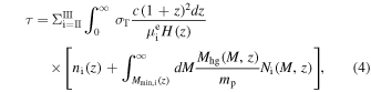
Thus, the evolution of luminous sources determines through Equations (1)–(3) the evolution of the IGM, and conversely, the evolution of the IGM determines in the way shown next the evolution of luminous sources, as well as the halo MF in regions with different ionization states (Manrique & Salvador-Solé 2015). Once the evolution of all these components has been determined we can calculate the CMB optical depth

and the Compton distortion y-parameter

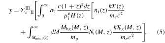
In Equations (4) and (5) H(z) is the Hubble parameter, ${\sigma }_{{\rm{T}}}$ is the photon Thomson scattering cross-section, c is the speed of light, ${M}_{\mathrm{hg}}(M,z)$ and ${T}_{\mathrm{hg}}(M,z)$ are the average mass and temperature of the hot gas in halos with mass M, respectively, ${N}_{{\rm{i}}}(M,z)\equiv {N}_{\mathrm{ion}}(M,z){Q}_{{\rm{i}}}(z)/({Q}_{\mathrm{II}}(z)+{Q}_{\mathrm{III}}(z))$ is the halo comoving abundance in region i, ${N}_{\mathrm{ion}}(M,z)$ being the halo MF in ionized regions, and ${M}_{\min ,{\rm{i}}}(z)$ is the minimum halo mass in region i able to trap gas, all of them dependent on z.

2.2. Luminous Sources

Halos grow through major mergers and smooth accretion. AMIGA follows this growth in a well-contrasted analytic manner with no free parameters (Salvador-Solé et al. 1998, 2007; Raig et al. 2001). This allows us to accurately calculate, at any given moment, their abundance (Juan et al. 2014a, 2014b) and inner structure and kinematics (Salvador-Solé et al. 2012a, 2012b), which in turn sets the structure and temperature of their hot gas (Solanes et al. 2005). The amount and metallicity of such a hot gas and the properties of the central galaxy and its satellites are monitored in AMIGA from the individual halo aggregation history.

As long as the hot gas has a metallicity below ${Z}_{{\rm{c}}}$ , molecular cooling takes place (see Manrique et al. 2015). When the temperature reaches a minimum value that cannot be surpassed, the cold gas accumulates in a central disk until the Bonnor–Ebert mass is reached. The cloud then collapses and fragments, giving rise to a small Pop III star cluster of about 1000 ${M}_{\odot }$ .¹⁰ The initial mass function (IMF) of Pop III stars is poorly known, but at the present stage we do not need it. We only need the mass fractions f₂ and f₃ of Pop III stars with masses in the ranges $130\leqslant {M}_{\star }/$ ${M}_{\odot }$ $\lt \,260$ , and ${M}_{\star }\gt 260$ ${M}_{\odot }$ , respectively. Indeed, stars in the former range explode in pair-instability SNe (PISNe), release about half their mass in metals, and do not leave any black hole as remnant, while those in the most massive range essentially collapse into a black hole without producing metals (Heger & Woosley 2002). Thus, the yield of massive Pop III stars, ${p}_{\mathrm{III}}$ , and the mass fraction of a Pop III star cluster ending up in a coalesced mini-MBH, ${\beta }_{\mathrm{III}}$ , satisfy the relations¹¹

On the other hand, the H i- and He ii-ionizing photon emissivities of massive Pop III stars depend on the mass fraction ${f}_{2}+{f}_{3}$ in a well-known way (Schaerer 2002).¹² Last, Pop III stars with masses below 130 ${M}_{\odot }$ contributing to the mass fraction ${f}_{1}=1-{f}_{2}-{f}_{3}$ behave like ordinary Pop II stars, except for their low metallicity. Therefore, the feedback of Pop III stars is fully determined by the mass fractions f₂ and f₃.

When the metallicity of the hot gas exceeds ${Z}_{{\rm{c}}}$ , it undergoes atomic cooling. The gas then contracts, keeping the initial angular momentum, and settles in a rotationally supported disk. The structure of disks is calculated according to Mo et al. (1998) from the specific angular momentum of the gas at the cooling radius, which equals that of DM as provided by numerical simulations. This leads to their effective (half-mass) radii ${r}_{{\rm{D}}}$ and central surface density 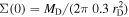${\rm{\Sigma }}(0)={M}_{{\rm{D}}}/(2\pi \,0.3\,{r}_{{\rm{D}}}^{2})$ , where ${M}_{{\rm{D}}}$ is the disk mass.¹³

If the disk is unstable, the cold gas is collected in a spheroid. Spheroids also form in galaxy mergers. Indeed, when a halo is captured by another one, it is truncated around the central galaxy, which becomes a satellite orbiting within the new halo. Satellites undergo dynamical friction and orbital decay, being eventually captured by the more massive central galaxy or merging with it if the mass ratio between the two objects is greater than 1:3. Satellites also interact between themselves and with the hot intrahalo gas. However, except for ram-pressure stripping, which is self-consistently calculated in AMIGA, these interactions (tidal stripping, gas starvation at the shock front of the hot gas, tidally induced disk-to-bulge mass transfer,…) are neglected in the present work as they should play no significant role at high-z when groups and clusters of galaxies are slightly developed and populated (but see Section 5.4).

Spheroids resulting from unstable disks or galaxy mergers have the Hernquist (1990) profile whose projection fits the ${r}^{1/4}$ law. Collisions between gas clouds yield the dissipative contraction of recently assembled spheroids with mass ${M}_{{\rm{B}}}$ as stars form, according to the physically motivated differential equation for the effective radius ${r}_{{\rm{B}}}$ (Manrique et al. 2015)

from the initial value given by the ${r}_{{\rm{B}}}\mbox{--}{M}_{{\rm{B}}}$ relation of non-contracted spheroids (see below) until the gas is exhausted or it reaches the density of molecular clouds ( $\sim {10}^{6}$ particles cm³). In Equation (8) ${M}_{\mathrm{cg},{\rm{B}}}(t)$ and ${Z}_{\mathrm{cg},{\rm{B}}}(t)$ are the mass and metallicity, respectively, of the cold gas in the spheroid at t, ${\tilde{\tau }}_{\mathrm{acc}}$ is the time elapsed from the formation of the spheroid to the quenching of star formation by the enlightened central AGN (see below), and ${\rho }_{\mathrm{dis}}$ is a characteristic gas density for the dissipative contraction of spheroids.

When the cold metal-rich gas falls into a galactic component C, i.e., a bulge (C = B) or a disk (C = D), new Pop II stars form. The SFR satisfies the usual Schmidt–Kennicutt law

where ${M}_{\mathrm{cg},{\rm{C}}}(t)$ is the mass of cold gas available, ${\tau }_{\mathrm{dyn},{\rm{C}}}$ is the dynamical timescale at the half-mass–radius of the galactic component, and ${\alpha }_{{\rm{G}}}$ is the star formation efficiency.

The amount of interstellar gas heated by SNe II in Pop II star formation episodes in the galactic component C is

where ${V}_{{\rm{C}}}$ is the circular velocity at ${r}_{{\rm{C}}}$ , ${V}_{\mathrm{hg}}$ is the typical thermal velocity of the hot gas in the halo where the heated gas is deposited, ${E}_{\mathrm{SN}}={10}^{51}$ erg is the typical energy liberated by one typical SN explosion, ${\eta }_{\mathrm{SN}}=0.014$ ${M}_{\odot }$ ⁻¹ is the number of such explosions per unit stellar mass in a typical ∼0.20 Gyr duration starburst for the adopted IMF, and ${\epsilon }_{{\rm{C}}}$ is the SN heating efficiency of the component. Due to the different SFR, and the geometry and porosity of the gas in spheroids and disks, ${\epsilon }_{{\rm{C}}}$ is let to take different values in bulges ( ${\epsilon }_{{\rm{B}}}$ ) and disks ( ${\epsilon }_{{\rm{D}}}$ ). Disks smaller than the corresponding spheroids are, however, assumed to be oblate pseudo-bulges with ${\epsilon }_{{\rm{B}}}$ .

The amount of intrahalo gas heated through PISN during the explosion of very massive Pop III stars and leaving the halo is also calculated according to Equation (10), but with ${\epsilon }_{{\rm{C}}}={\epsilon }_{{\rm{B}}}$ , ${E}_{\mathrm{SN}}={E}_{\mathrm{PISN}}={10}^{53}$ erg, ${\eta }_{\mathrm{SN}}={\eta }_{\mathrm{PISN}}=0.0015$ ${M}_{\odot }$ ⁻¹ (Heger & Woosley 2002; Schaerer 2002), ${V}_{{\rm{C}}}$ equal to the halo circular velocity at half-mass–radius, and ${V}_{\mathrm{hg}}=0$ .

The instantaneous emission at all the relevant wavelengths of normal galaxies is calculated according to their individual stellar formation and metallicity histories using the stellar population synthesis model (SPSM) by Bruzual & Charlot (2003) for the adopted IMF (see below) and taking into account the typical yield of Pop II stars (Vincenzo et al. 2016) and all the mass and metallicity exchanges between the different galaxy and halo components.

In particular, as long as halos accrete, the metal-enriched gas ejected from the central galaxy remains, due to viscosity, at the cooling radius where it is the next to cool. AMIGA assumes that, at the next major merger, all the hot gas of the progenitors is mixed up, except for their inner ${h}_{\mathrm{mix}}$ mass fraction, which retains all the reheated gas remaining in those progenitors. This means that metals ejected from central galaxies take at least two consecutive major mergers to get well mixed within the halo. As a consequence, the hot gas in the the inner part of the halo is always somewhat more metal-rich than in the outer part.

MBHs originate as remnants of the most massive Pop III stars that, as mentioned before, are supposed to coalesce in one mini-MBH per star cluster. When Pop III star clusters (or their remnants) are subsequently captured by normal galaxies and reach their spheroids, the corresponding mini-MBHs migrate by dynamical friction to their centers where they merge with the MBH lying there. MBHs at the center of spheroids progressively grow not only through mergers, but mainly through accretion of gas (and to a much lesser extent of stars). AMIGA does not assume any specific fraction of the gas fallen into spheroids to fuel the central MBH. Instead, it assumes that, each time new gas falls into a spheroid, part of it forms stars, and part fuels the MBH. The starburst lasts until it is quenched by the enlightened AGN that heats mechanically an amount of gas equal to

and expels it back into the halo through super-winds. In Equation (11) ${\epsilon }_{\mathrm{AGN}}$ is the so-called quasar-mode AGN heating efficiency, and $\langle L\rangle$ is the AGN bolometric luminosity L(t), averaged over the typical duration ( ${\tau }_{\mathrm{acc}}=0.15\,\mathrm{Gyr};$ Kelly et al. 2010) of one such enlightening episodes. The bolometric light curve is modeled according to Hatziminaoglou et al. (2003) through the expression

where ${V}_{\mathrm{last}}$ is the Keplerian velocity at the last marginally stable orbit (at 9.2 times the Schwarschild radius) around the MBH, and ${\dot{M}}_{\mathrm{BH}}$ is the time-derivative of the MBH accretion curve, ${M}_{\mathrm{BH}}(t)$ , assumed with a universal dimensionless bell-shaped form, whose maximum at ${\tau }_{\mathrm{acc}}$ sets the quenching of the starburst going on in the spheroid.

The fraction of H i- (and He ii-) ionizing photons escaping from halos with a virial temperature below 10⁴ K is self-consistently calculated by subtracting those photons ionizing the neutral intrahalo gas, taking into account recombinations. Above 10⁴ K, a fixed value, ${f}_{\mathrm{esc}}$ , is adopted, distinguishing between galaxies, ${f}_{\mathrm{esc},{\rm{G}}}$ , and AGNs, ${f}_{\mathrm{esc},\mathrm{AGN}}$ .

The fraction of the SN explosion energy converted to X-ray photons through free–free emission of the SN remnant and inverse Compton scattering of CMB photons by relativistic electrons is about 1% (Oh & Haiman 2003), and the fraction of the AGN bolometric luminosity emitted in soft X-rays is 4% (Vasudevan & Fabian 2007). About half of those soft X-ray photons Compton heat the IGM in neutral regions due to the residual free electrons. The other half produce secondary ionizations and excitations (Oh & Haiman 2003), neglected in AMIGA.

2.3. Parameters

All quantities entering the previous equations are self-consistently evolved in AMIGA from trivial initial conditions. Only a few of them must be supplied as external inputs.

Some of those external inputs correspond to reasonably well-known functions of redshift, stellar mass, or galaxy mass. These are the following.

1.
The clumping factor: Hydrodynamic simulations show that C(z) is equal to about 3 at $z\sim 6$ (Finlator et al. 2012 and references therein), and evolves essentially as
Strictly speaking, this fitting expression was derived by Finlator et al. (2012) from their simulations where reionization started at $z\sim 13$ , and ended up at ${z}_{\mathrm{ion},{\rm{H}}}\sim 8$ . In the real universe, ${z}_{\mathrm{ion},{\rm{H}}}$ is instead closer to $z\sim 6$ , and starts at a redshift ${z}_{\mathrm{start}}$ to be determined. We thus adopt the following generalization of expression (13),
with identical linear behavior but satisfying $C({z}_{\mathrm{start}})\equiv {C}_{{\rm{F}}}(13)=1$ and $C(6)\equiv {C}_{{\rm{F}}}(8)=3$ .
2.
The IMF of ordinary Pop II stars: Observations show that it can be approximated by a Salpeter IMF. In AMIGA we adopt the Salpeter slope, −2.35, for large masses up to 130 ${M}_{\odot }$ , and the slope −1 for small masses in the range $0.1\lt {M}_{\star }/{M}_{\odot }\lt 0.5$ . Such an IMF is consistent with the observed local one (Wilkins et al. 2008), and similarly top-heavy as the Chabrier (2003) IMF.
3.
The ${r}_{{\rm{B}}}\mbox{--}{M}_{{\rm{B}}}$ relation for non-dissipatively contracted spheroids: Assuming for simplicity that it is a power law, ${r}_{{\rm{B}}}={{AM}}_{{\rm{B}}}^{\gamma }$ , and taking into account that spheroids at the two mass ends of the observed relations for nearby objects (Phillips et al. 1997; Shen et al. 2003, 2007) have not suffered dissipative contraction,¹⁴ one is led to $A\approx 0.049$ Kpc ${M}_{\odot }$ ${}^{-\gamma }$ , and $\gamma \approx 0.20$ .

Even though there is some uncertainty in the preceding expressions, the results of the present study have been checked to be very robust against reasonable variations in the coefficients.

But most of the external inputs are constant or can be considered as such in a first approximation.¹⁵ Many of them are either well determined, as in the case of the threshold mass ratio for galaxy captures with destruction, the yield of Pop II stars, and the energy and frequency of SNe, or they play an insignificant role in the results, as the fraction of the energies released by SNe and AGNs that are converted into X-rays, so they can safely be taken with the fixed values specified in Section 2.2. Others can also be taken with any reasonable fixed value because their uncertainty is absorbed in other parameters. This is the case of the factors 0.5 and 1.0 in Equations (6)–(7), the constant ${\tilde{\tau }}_{\mathrm{acc}}$ in Equation (8), and the product ${V}_{\mathrm{last}}^{2}{\tau }_{\mathrm{acc}}$ times the factor arising from the universal dimensionless MBH accretion curve in Equation (11).

However, all the remaining external inputs must be left free since they are poorly determined, and have a significant effect on the results. These are thus the real parameters of the model to be adjusted through the fit to the observational data. Their complete list is the following:

${Z}_{{\rm{c}}}$ :	threshold metallicity for atomic cooling,
f₂:	mass fraction in intermediate Pop III stars,
f₃:	mass fraction in massive Pop III stars,
${\rho }_{\mathrm{dis}}$ :	characteristic density for dissipative contraction,
${\alpha }_{{\rm{G}}}$ :	Pop I and II star formation efficiency,
${\epsilon }_{{\rm{B}}}$ :	SN heating efficiency in spheroids,
${\epsilon }_{{\rm{D}}}$ :	SN heating efficiency in disks,
${\epsilon }_{\mathrm{AGN}}$ :	AGN quasar-mode heating efficiency,
${h}_{\mathrm{mix}}$ :	mixing hot gas mass fraction,
${f}_{\mathrm{esc},{\rm{G}}}$ :	escape fraction from galaxies, and
${f}_{\mathrm{esc},\mathrm{AGN}}$ :	escape fraction from AGN.

As we will see in Section 4, there is some degeneracy between these 11 parameters. In addition, the unknown Pop III star IMF must satisfy some conditions that have not yet been enforced. As a consequence we will end up with only nine degrees of freedom. Although this may still seem quite a large number, it is similar to that found in all recent analytic models of the EoR¹⁶ that find ${z}_{\mathrm{ion},{\rm{H}}}=6$ from the fit to the observed SFR density of galaxies at $z\gt 6$ (Bouwens et al. 2015; Ishigaki et al. 2015; Robertson et al. 2015). We remark, however, that our model is expected to recover not only the observed redshift of full hydrogen ionization, but the whole evolution of the universe from the fit to all the observed cosmic histories at $z\gt 2$ . Such an achievement with so few parameters is possible thanks to the fact that our model is self-consistent so that many quantities can be calculated and need not to be considered as free parameters.

3. THE OBSERVED HIGH-Z UNIVERSE

All the observational data currently available on the evolution of the universe at $z\gt 2$ (see Figure 1) refer to the following:

(a)
the cold gas mass density history (CGH),
(b)
the stellar mass density history (STH),
(c)
the MBH mass density history (MBHH),
(d)
the hot gas metallicity history (HGMH),
(e)
the cold gas metallicity history (CGMH),
(f)
the stellar metallicity history (STMH),
(g)
the IGM metallicity history (IGMMH),
(h)
the galaxy morphology history (GAMH),
(i)
the galaxy size history (GASH),
(j)
the SFR density history (SFH),
(k)
the H i-ionizing emissivity history (IEH), and
(l)
the IGM temperature history (IGMTH).

Figure 1. Refer to the following caption and surrounding text. — **Figure 1.** Cosmic histories with available data at $z\gt 2$ (see text for the different symbols in some panels): (a) cold gas mass densities (Péroux et al. 2003; Prochaska et al. 2005); (b) stellar mass densities (Reddy & Steidel 2009; Stark et al. 2009; González et al. 2010, 2011; Labbé et al. 2010a, 2010b; Caputi et al. 2011; Mortlock et al. 2011a); (c) MBH mass densities (Kelly et al. 2010; Willott et al. 2010a; Treister et al. 2011); (d) hot gas metallicities (Songaila 2001; Ryan-Weber et al. 2009; Simcoe et al. 2011; D’Odorico et al. 2013); (e) cold gas metallicities (Maiolino et al. 2008; Sommariva et al. 2012; Cullen et al. 2014); (f) stellar metallicities (Halliday et al. 2008; Sommariva et al. 2012); (g) IGM metallicities (based on estimates by Ryan-Weber et al. 2009; Simcoe et al. 2011; D’Odorico et al. 2013); (h) fraction of spheroid-dominated galaxies with masses $\gtrsim {10}^{11}$ ${M}_{\odot }$ (Buitrago et al. 2008; Bruce et al. 2014a); (i) median effective radii of spheroid-dominated galaxies (Buitrago et al. 2008); (j) SFR densities (Reddy & Steidel 2009; Lorenzoni et al. 2011; Bouwens et al. 2012b; Coe et al. 2013; Ellis et al. 2013; Oesch et al. 2013); (k) total ionizing emissivities (Becker & Bolton 2013) and the contribution from AGN (Cowie et al. 2009); and (l) IGM temperatures (Bolton et al. 2010, 2012; Lidz et al. 2010). Error bars are 1σ deviations, except for panel (g) where they give upper and lower limits. The density parameters are for the *current value* of the critical cosmic density, ${\rho }_{{\rm{c}}}(z=0)$ , and the scaling factors in the right column are ${r}_{0}={r}_{e}(z=0)$ , ${\dot{\rho }}_{0}=1$ ${M}_{\odot }$ yr⁻¹ Mpc⁻³, ${\dot{N}}_{0}={10}^{51}$ photons s⁻¹ Mpc⁻³, and ${T}_{0}={10}^{4}$ K. Other cosmic histories with no data also included for the densities and metallicities in the left and middle columns to cover all baryonic components: (x) hot gas mass densities, (y) IGM mass densities, and (z) metallicities of matter fallen into MBHs.
Download figure:
Standard image High-resolution image

**Figure 1.** Cosmic histories with available data at $z\gt 2$ (see text for the different symbols in some panels): (a) cold gas mass densities (Péroux et al. 2003; Prochaska et al. 2005); (b) stellar mass densities (Reddy & Steidel 2009; Stark et al. 2009; González et al. 2010, 2011; Labbé et al. 2010a, 2010b; Caputi et al. 2011; Mortlock et al. 2011a); (c) MBH mass densities (Kelly et al. 2010; Willott et al. 2010a; Treister et al. 2011); (d) hot gas metallicities (Songaila 2001; Ryan-Weber et al. 2009; Simcoe et al. 2011; D’Odorico et al. 2013); (e) cold gas metallicities (Maiolino et al. 2008; Sommariva et al. 2012; Cullen et al. 2014); (f) stellar metallicities (Halliday et al. 2008; Sommariva et al. 2012); (g) IGM metallicities (based on estimates by Ryan-Weber et al. 2009; Simcoe et al. 2011; D’Odorico et al. 2013); (h) fraction of spheroid-dominated galaxies with masses $\gtrsim {10}^{11}$ ${M}_{\odot }$ (Buitrago et al. 2008; Bruce et al. 2014a); (i) median effective radii of spheroid-dominated galaxies (Buitrago et al. 2008); (j) SFR densities (Reddy & Steidel 2009; Lorenzoni et al. 2011; Bouwens et al. 2012b; Coe et al. 2013; Ellis et al. 2013; Oesch et al. 2013); (k) total ionizing emissivities (Becker & Bolton 2013) and the contribution from AGN (Cowie et al. 2009); and (l) IGM temperatures (Bolton et al. 2010, 2012; Lidz et al. 2010). Error bars are 1σ deviations, except for panel (g) where they give upper and lower limits. The density parameters are for the *current value* of the critical cosmic density, ${\rho }_{{\rm{c}}}(z=0)$ , and the scaling factors in the right column are ${r}_{0}={r}_{e}(z=0)$ , ${\dot{\rho }}_{0}=1$ ${M}_{\odot }$ yr⁻¹ Mpc⁻³, ${\dot{N}}_{0}={10}^{51}$ photons s⁻¹ Mpc⁻³, and ${T}_{0}={10}^{4}$ K. Other cosmic histories with no data also included for the densities and metallicities in the left and middle columns to cover all baryonic components: (x) hot gas mass densities, (y) IGM mass densities, and (z) metallicities of matter fallen into MBHs.
Download figure:
Standard image High-resolution image

Taking into account that there are two independent IEHs, one for galaxies, and the other for AGNs, this represents 13 independent global, i.e., averaged or integrated, cosmic histories.¹⁷ In addition, the following differential properties are also available at a few discrete redshifts (see e.g., Figures 8 and 11):

(m)
the galaxy stellar MFs (or UV LFs), and
(n)
the MBH MFs (or AGN optical and X-ray LFs).

The mass density and emissivity estimates at different redshifts are derived from these MFs or LFs at the corresponding z, extrapolated beyond the observational limits.¹⁸ Therefore, these MFs or LFs harbor more information than the corresponding global properties above. However, they are harder to handle. Thus we will concentrate on trying to fit the former cosmic histories, and then check whether or not the galaxy and MBH MFs at a few representative redshifts are also well recovered.

We briefly discuss the techniques, approximations, and models used to infer all those data. All quantities given below refer to the Salpeter-like IMF adopted in AMIGA (applying the conversion factor from a strict Salpeter IMF provided by Wilkins et al. 2008) and to a Hubble constant of 67.3 km s⁻¹ Mpc⁻¹.

(a)
Cold gas mass densities are computed from the distribution function of H i column densities per unit redshift in damped Lyα systems (DLAs) in the spectra of quasars up to ${z}_{\mathrm{ion},{\rm{H}}}$ , integrated from zero to infinity. The estimates shown in panel (a) of Figure 1 were obtained by Péroux et al. (2003) and Prochaska et al. (2005). Note that some amount of H₂ (and other molecules), not accounted for in these estimates, must also be present. However, the real gas densities are not expected to be substantially greater.
(b)
Stellar mass densities are inferred by fitting the SED of high-z galaxies, obtained from several optical and infrared rest-frame bands, to template SEDs generated by SPSMs assuming an IMF and a dust absorption correction.¹⁹ The resulting galaxy stellar MFs are extrapolated down to 10⁸ ${M}_{\odot }$ . In panel (b) we show one illustrative sample of data sets obtained by several authors (Reddy & Steidel 2009; Stark et al. 2009; González et al. 2010, 2011; Labbé et al. 2010a, 2010b; Caputi et al. 2011; Mortlock et al. 2011a). The large scatter in the data is mostly due to the very uncertain correction for dust attenuation.
(c)
MBH masses at high redshifts are estimated by the method of reverberation mapping that assumes the broad line emitting clouds around AGNs are virialized. The largest uncertainty in those masses arises from the unknown geometry and inclination of the system, and is encapsulated in a virial factor (f_σ or ${f}_{\mathrm{FWHM}}$ , depending on whether the potential well is traced through the cloud velocity dispersion or the emission-line width, respectively) of the order of one. The MBH mass density estimates at $z\lt 5$ and z = 6.1 plotted as open circles in panel (c) have been computed using the MBH MFs derived by Kelly et al. (2010) and Willott et al. (2010a), respectively, from AGN LFs in rest-frame UV. These MFs are, however, greatly affected by AGN obscuration and inactivity, and are substantially lower than the filled circle at z = 6.5 inferred by Treister et al. (2011) from the extrapolated AGN LF in X-rays, less affected by these effects.²⁰ On the contrary, this latter estimate is fairly aligned with the filled circles at the previous redshifts, derived assuming a constant MBH-to-spheroid mass ratio, μ, equal to $8\times {10}^{-3}$ (Kormendy & Ho 2013, taking into account the change in IMF),²¹ and the upper envelope of the stellar mass densities given in item (b).²²
(d)
Absorption lines of metal ions, usually C iv, are observed outside the Lyα forest in the spectra of distant quasars. The absorbers have column densities N according to a distribution function at any given z well fitted by the expression $f(N)\propto {N}^{-(1.32+0.0779z)}$ (D’Odorico et al. 2013), from which one can infer the average metal abundance of the absorbers. The metallicities plotted in panel (d), obtained by Songaila (2001), Ryan-Weber et al. (2009), Simcoe et al. (2011), and D’Odorico et al. (2013), have been homogenized to the widest column density range available ( ${10}^{12}\mbox{--}{10}^{15}$ cm⁻²), converted to C abundances for a [C iv/C] abundance ratio of 0.05 appropriate to high column densities (Simcoe 2006), and then to metallicities assuming the C mass fraction of ejecta from ordinary Pop I and II stars given by Ryan-Weber et al. (2009). Indeed, the absorbers are believed to be neutral polluted gas regions around intervening halos, with density contrasts spanning from 10 to 100 in redshifts going from 6 to 2, respectively. Consequently, these metallicities should coincide with that of the hot gas in low-mass halos having accreted gas for the first time (i.e., with masses between the minimum trapping mass at that z and, say, 1 dex larger).
(e)
Gas-phase metallicities of high-z star-forming galaxies are derived from emission lines in their composite spectra. The estimates obtained for different metal ions are calibrated against each other, and converted to the [O/H] abundance ratio, then to the global metallicity, using the relation provided by Sommariva et al. (2012). In panel (e) we plot typical values obtained for small samples of galaxies with stellar masses above $\sim 5\times {10}^{9}$ ${M}_{\odot }$ at z around 3.5 and 2.2, respectively, inferred by Maiolino et al. (2008) and Cullen et al. (2014), and several individual values for a few galaxies with similar masses at the remaining redshifts inferred by Sommariva et al. (2012).
(f)
Stellar metallicities of high-z star-forming galaxies are derived similarly to the gas-phase metallicities in item (e) but from ion absorption lines. In panel (f) we plot the values obtained for a small sample of galaxies with stellar masses above $\sim 5\times {10}^{9}$ ${M}_{\odot }$ at z around 2.0 inferred by Halliday et al. (2008) and several individual values corresponding to a few galaxies with similar masses inferred by Sommariva et al. (2012).
(g)
There are no direct measures of the average IGM metallicities. However, we can put in panel (g) some upper and lower limits. Indeed, as mentioned in item (d), metal absorption lines outside the Lyα forest in the spectra of distant quasars would be produced by the polluted IGM around halos. Since the metallicity of those systems decreases with increasing z due to the increasing effect of galaxy ejecta, their values for the most distant systems ( $5\leqslant z\lt 6$ ) are the best upper limits to the average “primordial” (i.e., enriched by Pop III stars only) IGM metallicity we can have. For the present purposes, these metallicities are derived assuming a [C iv/C] abundance ratio of 0.5 (Ryan-Weber et al. 2009), appropriate to low column densities, and a carbon mass fraction of Pop III stars (model C in Schaerer 2002) as it corresponds to IGM polluted by Pop III stars only. On the other hand, the IGM metallicity can become lower than ${Z}_{{\rm{c}}}$ at low-z due to the lower metallicity-to-ionizing photon contribution of normal galaxies into the IGM compared to that of Pop III stars that dominate at high-z. A lower limit of $0.5\times {10}^{-4}$ ${Z}_{\odot }$ is thus an educated guess.
(h)
Morphological fractions are inferred from fitting a Sérsic (1968) law to galaxy surface-brightness profiles using circular apertures. This yields the Sérsic index, n, and the effective (half-light) radius, ${r}_{{\rm{e}}}$ , of the galaxy. Alternatively one can decompose the surface-brightness profile in a bulge and a disk. The fractions of spheroid-dominated star-forming galaxies with stellar masses $\sim {10}^{11}$ ${M}_{\odot }$ plotted in panel (h) were obtained by Buitrago et al. (2008) for a threshold Sérsic index value of $n\gt 2$ , and by Bruce et al. (2014a), at z = 2.5, for star-forming galaxies with bulge-to-total light ratios greater than 0.5. Both methods yield similar results.
(i)
Galaxy sizes depend on the galaxy morphology. The median effective radii of spheroid-dominated ( $n\gt 2$ ) and disk-dominated ( $n\leqslant 2$ ) objects scaled to the corresponding local values (Shen et al. 2003) for galaxies with stellar masses $\sim {10}^{11}$ ${M}_{\odot }$ plotted in panel (i) as filled circles and open circles, respectively, were obtained by Buitrago et al. (2008) for the same galaxy sample as used to draw the morphological fraction in item (h). The estimates inferred by Bruce et al. (2014b) directly using the effective radii of bulges and disks yield substantially different results and have not been considered. On the other hand, we will concentrate, from now on, in the effective radii of spheroid-dominated galaxies, as those of disk-dominated galaxies depend on the relative spatial distribution of stars and gas in the disk, which is not modeled in AMIGA.
(j)
SFR densities, ${\dot{\rho }}_{* }$ , are derived from the luminosity of observed galaxies in broadband or narrowband filters that traces active star formation, correcting for incompleteness from the extrapolated LFs and for dust absorption, applying IMF-dependent SFR calibrations. In panel (j) we plot the estimates inferred by Reddy & Steidel (2009), Lorenzoni et al. (2011), Bouwens et al. (2012b), Oesch et al. (2013), Coe et al. (2013), and Ellis et al. (2013). The dust-uncorrected values listed by Bouwens et al. (2012b) have been shifted upwards according to Jaacks et al. (2012) to correct for that effect. The resulting SFR densities are in very good agreement with the latest results published by McLeod et al. (2015).
(k)
Similarly to the escape fraction of ionizing (or Lyman-continuum, LyC) photons, which has two different versions, one for galaxies and the other for AGNs, we will distinguish between the H i-ionizing emissivity from normal galaxies and AGN. At high-z, the LyC emissivity of normal galaxies is usually estimated from their SFR densities assuming a given escape fraction of ionizing photons (Richard et al. 2006; Stark et al. 2007; Bouwens et al. 2011). These estimates are not considered here as they are equivalent to the SFR densities plotted in panel (h). An alternative method (Becker & Bolton 2013), independent from the SFR densities consists of using the Lyα effective optical depth inferred from the comparison of the observed Lyα forest with synthetic data obtained from hydrodynamic simulations, modeling photon mean free paths for the assumed ionizing emissivities. These are the estimates plotted as filled circles in panel (k). Regarding LyC emissivity from AGNs, this is estimated from UV observations of a large sample of X-ray AGNs. The results derived by Cowie et al. (2009) are plotted in the same panel as empty circles.
(l)
The temperature of the singly ionized IGM is usually derived from the small-scale structure of the Lyα forest, using hydrodynamic simulations and galaxy and quasar emission models. This is the case for the data at $z\lt 5$ derived by Lidz et al. (2010) plotted in panel (l). We do not include the estimates inferred by Becker et al. (2011) as they greatly depend on the poorly known density-temperature relation. Unfortunately, all those measures are extremely challenging for z approaching 6. An alternative method that sidesteps such a difficulty consists of probing the IGM temperature within a proper distance of ∼5 Mpc of quasars by combining the cumulative probability distribution of Doppler broadening and synthetic Lyα spectra. The measurements plotted at $z\sim 6$ were obtained in this way by Bolton et al. (2010) and Bolton et al. (2012), using one and seven quasars, respectively.
(m)
Galaxy stellar MFs are obtained from the galaxy LFs in rest-frame UV. The conversion involves the assumptions and procedures mentioned in item (b). For consistency, we adopt the MFs corrected for absorption inferred by González et al. (2011) at z = 3.8 and z = 6.8, which were also used to derive the stellar mass densities plotted in panel (b) at those redshifts that typically bracket the range of interest.
(n)
Similar comments hold for the MBH MFs. Their derivation from optical AGN LFs involves the assumptions and procedures mentioned in item (c). For consistency, we adopt the MFs inferred by Vestergaard et al. (2008) and Willott et al. (2010a) at z = 3.3 and z = 6.1, respectively, which were also used to infer the MBH mass densities plotted in panel (c) at those redshifts that bracket the range of interest.

4. FITTING STRATEGY

The goal is to adjust the 11 free parameters mentioned in Section 2 through the fit to the 13 independent cosmic histories described in Section 3, enforcing the constraints on ${z}_{\mathrm{ion},{\rm{H}}}$ and ${Q}_{{\rm{H}}{\rm{II}}}(z)$ mentioned in Section 1 as priors.

Scanning a whole 11 dimensional (11D) parameter space is not an easy task. Fortunately, we can take advantage of some particularities of the problem that greatly simplify the fitting procedure.

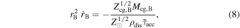
First, the characteristic dissipation density, ${\rho }_{\mathrm{dis}}$ , is fully constrained by the data, regardless of the value of any other parameter. Indeed, Equation (8) recovers the observed effective radius of massive spheroids at $z=2\mbox{--}3$ formed in major mergers of two galaxies with the typical gas content and metallicity (see panels (i), (a), and (e) of Figure 1) provided only $\mathrm{log}({\rho }_{\mathrm{dis}}$ ${M}_{\odot }$ ⁻¹ Kpc ${}^{3})=6.0\pm 0.6$ .

Second, the properties of normal galaxies and MBHs decouple from those of Pop III stars (Manrique et al. 2015). Indeed, massive Pop III stars lose metals through PISN-driven winds into the ionized bubbles they form around. When this polluted gas falls into halos and cools, normal galaxies form. In principle, the properties of those galaxies should thus depend on the metallicity of the ionized IGM set by Pop III stars through the values of ${Z}_{{\rm{c}}}$ , f₂, and f₃. But normal galaxies eject such large amounts of metals into the hot gas in halos through Type II SN- and AGN-driven winds that the hot gas rapidly loses the memory of its initial metallicity, and the properties of galaxies rapidly become independent of ${Z}_{{\rm{c}}}$ , f₂, and f₃. Similarly, MBHs are seeded by the remnants of massive Pop III stars. But the dramatic growth of MBHs within spheroids, regulated by the amount of gas reaching them, causes MBHs to rapidly lose the memory of their seeds, and the MBH properties also become independent of ${Z}_{{\rm{c}}}$ , f₂, and f₃. We can thus concentrate on adjusting, in a first step, the parameters referring to Pop III stars and, afterward, those referring to normal galaxies and MBHs. Notice that, even though the properties of the two kinds of sources are independent of each other, we cannot exchange the order of those fits. Some of the observables involving the parameters of the latter set refer to mean mass densities per unit volume, not per unit ionized volume, or to metallicities averaged over all regions, not over ionized regions. Consequently, they involve not only the properties of normal galaxies and MBHs, but also the volume filling factor of ionized regions, which depends on the mass fraction, ${f}_{2}+{f}_{3}$ , of massive Pop III stars. Nonetheless, once the parameters f₂ and f₃ are fixed, those observables will depend only on the parameters referring to normal galaxies and MBHs.

Third, most of the parameters in these two sets can be adjusted sequentially.

For a given value of ${Z}_{{\rm{c}}}$ , the ionization and photo-heating of the IGM at high-z depend only on the mass fraction ${f}_{2}+{f}_{3}$ of massive Pop III stars, while the mass of metals ejected in ionized regions depends only on the mass fraction f₂. Thus it should be possible to adjust ${f}_{2}+{f}_{3}$ by fitting the IGMTH at high-z, and then adjust f₂ by fitting the IGMMH also at high-z.

On the other hand, for a given couple of ${\epsilon }_{{\rm{B}}}$ and ${\epsilon }_{{\rm{D}}}$ values, the amount of gas in the disk or spheroid of a galaxy at any moment is equal to the amount of gas fallen into it, which depends on cosmology (through the halo characteristics, the hot gas cooling rate, and the galaxy merger rate),²³ minus the amount of gas used to form stars and ejected from the component (the latter depending on the former).²⁴ The inductive reasoning thus implies that the stellar masses of normal galaxies depend only on ${\alpha }_{{\rm{G}}}$ . Similarly, the mass of gas fueling the central MBH of a galaxy depends on the gas mass collected in the spheroid, which together with the stellar mass sets the dynamics, and hence, the mass of newly formed stars and of gas heated by SNe, the mass of the MBH determining its accretion rate, and the mass of gas heated by the enlightened AGNs. Therefore, the inductive reasoning implies that the MBHH depends on both ${\alpha }_{{\rm{G}}}$ and ${\epsilon }_{\mathrm{AGN}}$ . Last, the metallicity of the hot gas in the halo that determines, through the gas cooling and the metal-enriched gas ejected from galaxies, the cold gas, and stellar metallicities of those objects depends on cosmology, on ${\alpha }_{{\rm{G}}}$ and ${\epsilon }_{\mathrm{AGN}}$ , and on ${h}_{\mathrm{mix}}$ setting the mixing rate of the reheated gas in the halo. Finally, the emissivity of galaxies and AGNs depends on all the previous parameters setting the whole evolution of galaxies and AGNs and their respective intrinsic ionizing photon production rates and the values of ${f}_{\mathrm{esc}}$ from the two kinds of sources. Consequently, it should be possible to adjust ${\alpha }_{{\rm{G}}}$ by fitting the SFH (or STH), then ${\epsilon }_{\mathrm{AGN}}$ by fitting the MBHH, then ${h}_{\mathrm{mix}}$ by fitting the HGMH (or any of the CGMH and STMH), and last the ${f}_{\mathrm{esc}}$ values of galaxies and AGNs by fitting their corresponding IEHs with the suited priors on ${z}_{\mathrm{ion},{\rm{H}}}$ and ${d}_{z}{Q}_{{\rm{H}}{\rm{II}}}$ (hereafter ${d}_{z}$ means z-derivative).

Of course, this sequential fitting procedure should be carried out for every possible set of ${Z}_{{\rm{c}}}$ , ${\epsilon }_{{\rm{B}}}$ , and ${\epsilon }_{{\rm{D}}}$ values in the corresponding three-dimensional space. But this is a minor difficulty compared to directly looking for acceptable solutions in the whole 11D parameter space.

Any “acceptable solution” should thus fit with acceptable ${\chi }^{2}$ values the IGMMH, the IGMTH, the SFH (and the STH), the MBHH, the HGMH (and the CGMH and STMH), and the IEHs for galaxies and AGNs, with ${z}_{\mathrm{ion},{\rm{H}}}={6.0}_{-0.5}^{+0.3}$ and ${d}_{z}{Q}_{{\rm{H}}{\rm{II}}}(z=7)\lt 0$ . Moreover, since ${\epsilon }_{{\rm{B}}}$ and ${\epsilon }_{{\rm{D}}}$ govern the amount of cold gas remaining in disks and of stars forming in spheroids, the CGH and GAMH should hopefully also be fitted. And given the way ${\rho }_{\mathrm{dis}}$ is determined, the GASH should too. In principle, the solution so obtained should also recover the observed galaxy stellar and MBH MFs and, provided ${Z}_{{\rm{c}}}$ is not degenerate so that there is still one degree of freedom to play with, we may expect the solution to also fulfill the constraints on $\tau$ and y. Thus the problem is not only well posed, but in principle also slightly overdetermined.

Unfortunately, the IGMMH and IGMTH at high-z are not well constrained. The only available data on the IGM temperature refer to $z\lesssim 6$ where Pop III stars play no significant role, and there are just a few loose bounds for the IGM metallicity. Consequently, f₂ and f₃ cannot be determined in the previous simple manner. Moreover, ${Z}_{{\rm{c}}}$ is degenerate with f₂ and f₃. The good news is that this degeneracy reduces the degrees of freedom to 10, which facilitates the fit at the cost, of course, of making it even harder to find any acceptable solution.

Indeed, massive Pop III stars are the first source of ionizing photons, with emissivity equal to ${m}_{{\rm{p}}}{\xi }_{\mathrm{III}}({f}_{2}+{f}_{3}){\dot{M}}_{\mathrm{III}}$ , where ${\dot{M}}_{\mathrm{III}}$ and ${\xi }_{\mathrm{III}}$ are the formation rate and LyC photon production rate of Pop III stars, respectively. Those stars also pollute with metals the ionized bubbles at the rate $0.5{f}_{2}{\dot{M}}_{\mathrm{III}}$ . Therefore, the formation of normal galaxies is possible provided the metallicity of such bubbles, $0.5{f}_{2}/[{m}_{{\rm{p}}}{\xi }_{\mathrm{III}}({f}_{2}+{f}_{3})]$ , is greater than ${Z}_{{\rm{c}}}$ . But this condition is necessary although not sufficient. When normal galaxies form, they keep on ionizing and photo-heating the surrounding IGM, while they lose very few metals into it (they rather enrich the hot intrahalo gas). Consequently, the metallicity of ionized bubbles decreases, and their temperature increases, so the formation of new galaxies may be quenched, and reionization may be aborted. Only if the initial IGM metallicity is sufficiently large will the formation of normal galaxies last long enough for reionization to proceed successfully.

According to the previous discussion, the evolution of the universe for some values ${Z}_{{\rm{c}}}$ , f₂, and f₃ will thus be essentially the same (with ${Z}_{\mathrm{IGM}}$ in units of ${Z}_{{\rm{c}}}$ ) as for other values ${Z}_{{\rm{c}}}^{\prime }$ , ${f}_{2}^{\prime }$ , and ${f}_{3}^{\prime }$ , provided the IGM reionization and metal-enrichment histories driven by Pop III stars are the same, that is, provided the two sets of values satisfy the relations

This leads to the following simple fitting procedure. For some fiducial values of ${Z}_{{\rm{c}}}$ , and ${f}_{2}/({f}_{2}+{f}_{3})$ warranting that reionization will not be aborted, we scan all possible values of f₃, ${\epsilon }_{{\rm{B}}}$ , and ${\epsilon }_{{\rm{D}}}$ , and for each set of these three values we adjust ${\alpha }_{{\rm{G}}}$ , ${\epsilon }_{\mathrm{AGN}}$ , ${h}_{\mathrm{mix}}$ , and ${f}_{\mathrm{esc}}$ in the sequential manner explained above, with the priors on ${z}_{\mathrm{ion},{\rm{H}}}$ and ${d}_{z}{Q}_{{\rm{H}}{\rm{II}}}$ . Then, given any acceptable solution, the relations (15) and (16) provide with any other combination of ${Z}_{{\rm{c}}}$ , f₂, and f₃ values leading to it. Last, we can check the values of τ and y as well as the right behavior of the galaxy stellar and MBH MFs.

4.1. Additional Constraints on the Pop III Star IMF

Were the Pop III star IMF known, we could readily calculate the mass fractions f₂ and f₃, and, as a bonus, leave the above-mentioned degeneracy. Unfortunately, such an IMF is poorly determined. But we can still enforce some conditions such an IMF must satisfy in order to further constrain the problem and reduce the degrees of freedom to 9 (8 if we discount ${\rho }_{\mathrm{dis}}$ , directly determined by the data).

The IMF of Pop III stars must be top-heavier than the IMF of ordinary stars (Larson 1998).²⁵ Approximating it by a power law $f({M}_{\star })\propto {M}_{\star }^{-{\alpha }_{\mathrm{III}}}$ like the Salpeter IMF, this implies either that ${\alpha }_{\mathrm{III}}$ is smaller than the Salpeter slope, 2.35, or that the upper or lower stellar masses are larger than for ordinary stars, i.e., ${M}_{\mathrm{III}}^{\mathrm{lo}}\gt 0.5$ ${M}_{\odot }$ and ${M}_{\mathrm{III}}^{\mathrm{up}}\gt 130$ ${M}_{\odot }$ ,²⁶ or both conditions at the same time.

But this is not all. The fact that the slope of the IMF for ordinary Pop I and II stars appears to be little sensitive to their metallicity indicates that ${\alpha }_{\mathrm{III}}$ should not be substantially smaller than 2.35;²⁷ i.e., it should be larger than 2.25 or at most larger than 2.15. On the other hand, ${M}_{\mathrm{III}}^{\mathrm{lo}}$ should be smaller than 260 ${M}_{\odot }$ , otherwise Pop III stars would not enrich with metals the IGM, and ${M}_{\mathrm{III}}^{\mathrm{up}}$ should be larger than 260 ${M}_{\odot }$ , otherwise Pop III stars would not seed MBHs, and smaller than 500 ${M}_{\odot }$ or at most smaller than 1000 ${M}_{\odot }$ (Heger & Woosley 2002; Schaerer 2002).

To account for all these restrictions parameters, f₂ and f₃ in the fitting procedure described above must be replaced by the equivalent ones (for a fixed ${\alpha }_{\mathrm{III}}$ value) ${M}_{\mathrm{III}}^{\mathrm{lo}}$ and ${M}_{\mathrm{III}}^{\mathrm{up}}$ parameters. Specifically, for some fiducial values of ${Z}_{{\rm{c}}}$ in the range $[{10}^{-5}$ ${Z}_{\odot },{10}^{-3}$ ${Z}_{\odot }]$ , of ${\alpha }_{\mathrm{III}}$ in the range [2.25, 2.35] (or [2.15, 2.35]), and of ${M}_{\mathrm{III}}^{\mathrm{up}}$ in the range [260 ${M}_{\odot }$ , 500 ${M}_{\odot }$ ] (or [260 ${M}_{\odot }$ , 1000 ${M}_{\odot }$ ]) warranting that reionization is not aborted, we scan all possible values of ${M}_{\mathrm{III}}^{\mathrm{lo}}$ in the range [0.5 ${M}_{\odot }$ , 130 ${M}_{\odot }$ ], and of ${\epsilon }_{{\rm{B}}}$ and ${\epsilon }_{{\rm{D}}}$ in the range $[0,1]\times [0,1]$ , and adjust in the sequential manner explained above the parameters ${\alpha }_{{\rm{G}}}$ , ${\epsilon }_{\mathrm{AGN}}$ , ${h}_{\mathrm{mix}}$ , and the two ${f}_{\mathrm{esc}}$ (see Figure 2), with the priors on ${z}_{\mathrm{ion},{\rm{H}}}$ and ${d}_{z}{Q}_{{\rm{H}}{\rm{II}}}$ . Using the relations (15) and (16), we find all sets of ${Z}_{{\rm{c}}}$ , ${\alpha }_{\mathrm{III}}$ , ${M}_{\mathrm{III}}^{\mathrm{up}}$ , and ${M}_{\mathrm{III}}^{\mathrm{lo}}$ values leading to every acceptable solution. Last, we check whether or not the constraints on $\tau$ and y are also fulfilled, and whether or not the observed galaxy stellar and MBH MFs are well recovered.

Figure 2. Refer to the following caption and surrounding text. — **Figure 2.** Fitting procedure making use of the Pop III star IMF and some fiducial values of ${Z}_{{\rm{c}}}$ , ${\alpha }_{\mathrm{III}}$ , and ${M}_{\mathrm{III}}^{\mathrm{up}}$ .
Download figure:
Standard image High-resolution image

**Figure 2.** Fitting procedure making use of the Pop III star IMF and some fiducial values of ${Z}_{{\rm{c}}}$ , ${\alpha }_{\mathrm{III}}$ , and ${M}_{\mathrm{III}}^{\mathrm{up}}$ .
Download figure:
Standard image High-resolution image

The result will depend, of course, on the somewhat uncertain masses (130 ${M}_{\odot }$ and 260 ${M}_{\odot }$ ) delimiting the ranges where Pop III stars have distinct behaviors. But this is a small drawback compared to the gain of better constraining ${Z}_{{\rm{c}}}$ and the Pop III star IMF.

5. RESULTS

Following this fitting procedure, we have looked for any possible solution, in the sense of being compatible with the currently available data on the high-z universe and the usual reionization constraints, and checked whether it has single or multiple reionization episodes.

The idea of double reionization was advocated by several authors (Cen 2003; Chiu et al. 2003; Haiman & Holder 2003; Hui & Haiman 2003; Naselsky & Chiang 2004; Sokasian et al. 2004; Furlanetto & Loeb 2005) to reconcile the apparent inconsistency between the value of the redshift of complete hydrogen ionization obtained from the spectra of distant sources ( ${z}_{\mathrm{ion},{\rm{H}}}\sim 6;$ Becker et al. 2001; Djorgovski et al. 2001) with that found from the CMB optical depth derived from the first-year WMAP data ( ${z}_{\mathrm{ion},{\rm{H}}}\gt 15$ as implied by $\tau =0.17;$ Kogut et al. 2003). Subsequent CMB-based measurements decreased this latter estimate until the present value of ${z}_{\mathrm{ion},{\rm{H}}}$ of about 10. In addition, it became clear that an instantaneous reionization event at $z\sim 10$ was not necessarily inconsistent with reionization being completed by ${z}_{\mathrm{ion},{\rm{H}}}\sim 6$ . Consequently, the double reionization scenario lost its interest. However, the possibility that reionization is double still remains. As a matter of fact, this is quite natural to expect.

Indeed, Pop III star clusters have a typical mass of $\sim {10}^{3}$ ${M}_{\odot }$ , which is much lower than the mass $\sim {10}^{6}$ ${M}_{\odot }$ of the most abundant dwarf galaxies at high redshifts (see below). However, massive Pop III stars emit 40–80 times more ionizing photons than normal O, B stars, so both kinds of sources compete in the IGM reionization. What is the dominant contribution? Pop III stars are the first to form, so they necessarily drive the initial ionization phase. And, since neutral pristine regions progressively disappear, the final ionization phase will be driven by normal galaxies. The SFR of Pop III stars is fully determined by cosmology, and their more or less top-heavy IMF depends on the unknown value of ${M}_{\mathrm{III}}^{\mathrm{lo}}$ (for the fiducial values of ${\alpha }_{\mathrm{III}}$ and ${M}_{\mathrm{III}}^{\mathrm{up}}$ ). Whereas the IMF of Pop I & II stars, set by the physics of protostellar clouds, is well determined, and their more or less intense SFR depends on the unknown value of ${\alpha }_{{\rm{G}}}$ . Consequently, the answer to the question above depends on the relative values of the two independent parameters ${M}_{\mathrm{III}}^{\mathrm{lo}}$ and ${\alpha }_{{\rm{G}}}$ . For the ${\alpha }_{{\rm{G}}}$ value giving good fits to the SFH of galaxies, the larger the value of ${M}_{\mathrm{III}}^{\mathrm{lo}}$ , the earlier Pop III stars will begin to ionize the IGM, and the more probable will be the double reionization scenario.

5.1. Reionization History

Figure 3 shows the reionization histories of the only acceptable solutions we find. They are concentrated in two narrow sets, one with one single hydrogen ionization episode at $z\sim 6$ , and the other one with two ionization episodes at $z\sim 10$ and $z\sim 6$ , separated by a short recombination period. The best solutions of the two kinds, i.e., those that provide the best fit to the data on the SFH, MBHH, HGMH, IEHs, GAMH, and GASH with the priors ${z}_{\mathrm{ion},{\rm{H}}}=6.0$ and ${d}_{z}{Q}_{{\rm{H}}{\rm{II}}}(z=7)\lt 0$ , are hereafter referred to as “S” (for single reionization) and “D” (for double reionization).

Figure 3. Refer to the following caption and surrounding text. — **Figure 3.** Only acceptable solutions with single (left panel) and double (right panel) reionization. In thick lines models S and D give the best solution of the respective types. In thin lines the solutions bracket the two sets. The error bars centered at z = 2.5 and z = 8.8 along ${Q}_{{\rm{S}}{\rm{II}}}=1.0$ give the estimated limits for the redshifts of complete helium and hydrogen ionizations, respectively (see Section 1); the vertical dotted black line marks the redshift z = 7 where ${Q}_{{\rm{H}}{\rm{II}}}$ is found to decrease with increasing z. (In the online journal, the solutions for single and double reionization in all the following figures in are in red and green, respectively.)
Download figure:
Standard image High-resolution image

**Figure 3.** Only acceptable solutions with single (left panel) and double (right panel) reionization. In thick lines models S and D give the best solution of the respective types. In thin lines the solutions bracket the two sets. The error bars centered at z = 2.5 and z = 8.8 along ${Q}_{{\rm{S}}{\rm{II}}}=1.0$ give the estimated limits for the redshifts of complete helium and hydrogen ionizations, respectively (see Section 1); the vertical dotted black line marks the redshift z = 7 where ${Q}_{{\rm{H}}{\rm{II}}}$ is found to decrease with increasing z. (In the online journal, the solutions for single and double reionization in all the following figures in are in red and green, respectively.)
Download figure:
Standard image High-resolution image

In all the solutions, the reionization of He ii also shows two distinct phases separated by a short recombination period. The first phase leads to a maximum in the volume fraction of He ii-ionized regions, although without complete ionization, at $z\sim 10$ in the solutions with double hydrogen reionization, and at $z\sim 6\mbox{--}7$ in the solutions with single hydrogen reionization. The first phase is also driven by Pop III stars, but the second one, completed at ${z}_{\mathrm{ion},\mathrm{He}}\sim 2.8$ , is driven by AGNs instead of normal galaxies. Thus, the He ii reionization history confirms the idea that, when two independent ionizing sources with distinct timing are at play, it is natural to have a non-monotonous reionization.

Table 1 lists the values of ${M}_{\mathrm{III}}^{\mathrm{lo}}$ , ${\epsilon }_{{\rm{B}}}$ , ${\epsilon }_{{\rm{D}}}$ , ${\alpha }_{{\rm{G}}}$ , ${\epsilon }_{\mathrm{AGN}}$ , ${h}_{\mathrm{mix}}$ , ${f}_{\mathrm{esc},{\rm{G}}}$ , and ${f}_{\mathrm{esc},\mathrm{AGN}}$ defining models S and D for the fiducial values of ${Z}_{{\rm{c}}}$ , ${\alpha }_{\mathrm{III}}$ , and ${M}_{\mathrm{III}}^{\mathrm{up}}$ given in Table 2. The errors in ${M}_{\mathrm{III}}^{\mathrm{lo}}$ delimit the acceptable solutions around models S and D; those in ${\epsilon }_{{\rm{B}}}$ and ${\epsilon }_{{\rm{D}}}$ mark the deviations from the best values of these two parameters still leading to acceptable solutions; and the errors in the remaining parameters are $1\sigma$ deviations from their best values in models S and D, estimated from the ${\chi }^{2}$ -test of their respective fits. In principle, the degeneracy between ${Z}_{{\rm{c}}}$ and the Pop III star IMF could cause the value of ${M}_{\mathrm{III}}^{\mathrm{lo}}$ to vary from that quoted in Table 1. But, for the reasons explained next, there is actually not much room for the possible values of ${Z}_{{\rm{c}}}$ , ${\alpha }_{\mathrm{III}}$ , and ${M}_{\mathrm{III}}^{\mathrm{up}}$ , which should thus be close to those given in Table 2.

Table 1. Values of the Adjusted Free Parameters (besides ${\rho }_{\mathrm{dis}}={10}^{6}$ ${M}_{\odot }$ Kpc ${}^{-3}$ ) for the Fiducial Values of the Degenerate Ones

Model	${M}_{\mathrm{III}}^{\mathrm{lo}}/{M}_{\odot }$	${\epsilon }_{{\rm{B}}}$	${\epsilon }_{{\rm{D}}}$	${\alpha }_{{\rm{G}}}$	${\epsilon }_{\mathrm{AGN}}$	${h}_{\mathrm{mix}}$	${f}_{\mathrm{esc},{\rm{G}}}$	${f}_{\mathrm{esc},\mathrm{AGN}}$
	[0.5, 260]	[0, 1]	[0, 1]	[0, 1]	[0, 1]	[0, 1]	[0, 1]	[0, 1]
S	${38}_{-7}^{+5}$	${1.00}_{-0.05}^{+0.00}$	${0.00}_{-0.00}^{+0.05}$	0.33 ± 0.11	0.0016 ± 0.0003	0.4 ± 0.3	0.053 ± 0.007	0.0053 ± 0.0006
D	${87}_{-6}^{+9}$	${1.00}_{-0.05}^{+0.00}$	${0.00}_{-0.00}^{+0.05}$	0.19 ± 0.04	0.0025 ± 0.0004	0.4 ± 0.3	0.055 ± 0.008	0.0053 ± 0.0005

Download table as: ASCII Typeset image

Table 2. Fiducial Values of the Degenerate Free Parameters

Model	$\mathrm{log}({Z}_{{\rm{c}}}/{Z}_{\odot })$	${\alpha }_{\mathrm{III}}$	${M}_{\mathrm{III}}^{\mathrm{up}}/$ ${M}_{\odot }$
		[2.15, 2.35]	[260, 1000]
S	−4.6 ± 0.1	${2.35}_{-0.10}^{+0.00}$	${300}_{-40}^{+0}$
D	−4.0 ± 0.1	${2.35}_{-0.10}^{+0.00}$	${300}_{-40}^{+0}$

Download table as: ASCII Typeset image

All the combinations of ${Z}_{{\rm{c}}}$ , ${\alpha }_{\mathrm{III}}$ , ${M}_{\mathrm{III}}^{\mathrm{up}}$ , and ${M}_{\mathrm{III}}^{\mathrm{lo}}$ leading to any given solution can be obtained from one particular combination leading to that solution and Equations (15) and (16) through the relations between the couples of ${M}_{\mathrm{III}}^{\mathrm{lo}}$ and ${M}_{\mathrm{III}}^{\mathrm{up}}$ , and f₂ and f₃ values for a given ${\alpha }_{\mathrm{III}}$ value. That degeneracy is shown in Figure 4. See also Figure 5 for the degeneracy in ${Z}_{{\rm{c}}}$ , f₂, and f₃. Since the minimum possible value of ${f}_{2}/({f}_{2}+{f}_{3})$ for reionization not to be aborted depends on ${Z}_{{\rm{c}}}$ , and, for a given ${\alpha }_{\mathrm{III}}$ , ${f}_{2}/({f}_{2}+{f}_{3})$ is a function of ${M}_{\mathrm{III}}^{\mathrm{up}}$ alone, there is also a one-to-one correspondence between the maximum possible value of ${M}_{\mathrm{III}}^{\mathrm{up}}$ and ${Z}_{{\rm{c}}}$ . Notice that, for the reasons explained in Section 5.3, the maximum possible value of ${M}_{\mathrm{III}}^{\mathrm{up}}$ for each ${Z}_{{\rm{c}}}$ is smaller in single than in double reionization. Specifically, it is equal to the maximum ${M}_{\mathrm{III}}^{\mathrm{up}}$ value found in double reionization times 0.85/0.21, where 0.21 and 0.85 are the minimum ${f}_{2}/({f}_{2}+{f}_{3})$ values in single and double reionization, respectively.

Figure 4. Refer to the following caption and surrounding text. — **Figure 4.** Degeneracy in ${Z}_{{\rm{c}}}$ , ${\alpha }_{\mathrm{III}}$ , ${M}_{\mathrm{III}}^{\mathrm{lo}}$ , and ${M}_{\mathrm{III}}^{\mathrm{up}}$ leading to the same solutions with single (lower lines) and double (upper lines) reionization (solid lines for the best solutions and dashed lines for the respective bracketing solutions) for ${\alpha }_{\mathrm{III}}$ equal to 2.35 (thick lines) and 2.25 (thin lines). The vertical black dotted lines mark the maximum possible ${M}_{\mathrm{III}}^{\mathrm{up}}$ values for the quoted logarithms of ${Z}_{{\rm{c}}}$ in double reionization (upper values), and single reionization (lower values).
Download figure:
Standard image High-resolution image

Figure 5. Refer to the following caption and surrounding text. — **Figure 5.** Same degeneracy (with the solutions for single reionization on the right and those for double reionization on the left) as in Figure 4 in terms of ${Z}_{{\rm{c}}}$ , f₂, and f₃. The black dot-dashed line, with equation ${f}_{2}+{f}_{3}=1$ , delimits the region with possible solutions. The diagonal black dotted lines mark the minimum possible ${f}_{2}/({f}_{2}+{f}_{3})$ values for the quoted logarithms of ${Z}_{{\rm{c}}}$ in double reionization (outer values), and single reionization (inner values).
Download figure:
Standard image High-resolution image

As shown in Figure 4, the upper limit of ${Z}_{{\rm{c}}}$ set by the lower limit of ${M}_{\mathrm{III}}^{\mathrm{up}}$ equal to 260 ${M}_{\odot }$ is ${10}^{-3.93}$ ${Z}_{\odot }$ in double reionization, and ${10}^{-4.53}$ ${Z}_{\odot }$ in single reionization. Whereas the lower limit set by the upper limit of ${M}_{\mathrm{III}}^{\mathrm{up}}$ equal to 500 ${M}_{\odot }$ (1000 ${M}_{\odot }$ ) is ${10}^{-4.17}$ ${Z}_{\odot }$ ( ${10}^{-4.30}$ ${Z}_{\odot }$ ) in double reionization, and ${10}^{-4.77}$ ${Z}_{\odot }$ ( ${10}^{-4.90}$ ${Z}_{\odot }$ ) in single reionization. 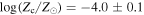Therefore, the central value and allowed range in double reionization are: $\mathrm{log}({Z}_{{\rm{c}}}/{Z}_{\odot })=-4.0\pm 0.1$ ${Z}_{\odot }$ , whereas in single reionization they are: 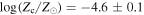$\mathrm{log}({Z}_{{\rm{c}}}/{Z}_{\odot })=-4.6\pm 0.1$ . These are the fiducial values of ${Z}_{{\rm{c}}}$ adopted for the fit. Note that, in the case of double reionization, the observed properties of the high-z universe imply a value of ${Z}_{{\rm{c}}}$ of 10⁻⁴ ${Z}_{\odot }$ , which coincides with that preferred on pure theoretical grounds (Santoro & Shull 2006; Smith et al. 2009; Schneider & Omukai 2010). Instead, in the case of single reionization, they imply a value of ${Z}_{{\rm{c}}}$ closer to the lower limit of 10⁻⁵ ${Z}_{\odot }$ .

In Figure 4 we also see that the degeneracy track associated with any given solution depends slightly on ${\alpha }_{\mathrm{III}}$ , and so does the exact upper limit of ${Z}_{{\rm{c}}}$ . But, for all reasonable values of ${\alpha }_{\mathrm{III}}$ , this dependence is only significant for unrealistic values of ${M}_{\mathrm{III}}^{\mathrm{up}}$ close to 1000 ${M}_{\odot }$ . We can thus adopt ${\alpha }_{\mathrm{III}}=2.35$ without any loss of generality, even though the true value of this parameter could be somewhat smaller.

Of course, all ${M}_{\mathrm{III}}^{\mathrm{up}}$ values smaller than the maximum possible value for a given ${Z}_{{\rm{c}}}$ (i.e., on the left of the corresponding vertical line in Figure 4) together with the ${M}_{\mathrm{III}}^{\mathrm{lo}}$ value associated with it along the degeneracy track yield essentially the same solution. (In Figure 5 all the couples f₂ and f₃ along the degeneracy track upward of that value of ${Z}_{{\rm{c}}}$ also lead to the same solution.) But the maximum possible value of ${M}_{\mathrm{III}}^{\mathrm{up}}$ in both single and double reionization, 300 ${M}_{\odot }$ , is already close to the lower limit of 260 ${M}_{\odot }$ , so the true value of ${M}_{\mathrm{III}}^{\mathrm{up}}$ must be close, indeed, to the fiducial one of 300 ${M}_{\odot }$ .

Having fixed the values ${Z}_{{\rm{c}}}$ , ${\alpha }_{\mathrm{III}}$ , and ${M}_{\mathrm{III}}^{\mathrm{up}}$ , the central and limiting values of ${M}_{\mathrm{III}}^{\mathrm{lo}}$ given in Table 1 have been obtained as follows. In the single reionization case, the best solutions they define have the central and limiting values of ${z}_{\mathrm{ion},{\rm{H}}}$ , equal to ${6.0}_{-0.5}^{+0.3}$ , the condition ${d}_{z}{Q}_{{\rm{H}}{\rm{II}}}\lt 0$ at z = 7 being automatically fulfilled in this case. In the double reionization case, the best solutions they define have ${z}_{\mathrm{ion},{\rm{H}}}={6.0}_{-0.5}^{+0.3}$ , but, in addition, the minimum of ${Q}_{{\rm{H}}{\rm{II}}}(z)$ is at a redshift larger than, although as close as possible to, z = 7. This warrants ${d}_{z}{Q}_{{\rm{H}}{\rm{II}}}\lt 0$ at z = 7 as wanted, together with the minimum possible redshift of first complete ionization, which is very convenient to have the smallest possible value of $\tau$ (see below).

The values of ${\epsilon }_{{\rm{B}}}$ and ${\epsilon }_{{\rm{D}}}$ are well constrained by the observed GAMH and GASH, as expected. In fact, those two properties appear to be extremely sensitive to small changes in the values of these (as well as other) parameters. Their values close to one and zero, respectively, in the two models agree with the results of analytic and hydrodynamic studies on the effects of SN heating (e.g., Dekel & Silk 1986; Mac Low & Ferrara 1999; Strickland & Stevens 2000), and they are also consistent with some properties of the nearby universe such as the high abundance of α-elements in the hot gas of halos or the correlations between the metallicity of the hot gas and the abundances of early- and late-type galaxies in galaxy clusters, indicative that most gas outflows take place from spheroids (e.g., Silk 1997).

The values of ${\alpha }_{{\rm{G}}}$ and ${\epsilon }_{\mathrm{AGN}}$ are also well constrained by the observed SFH and MBHH. The larger value of ${\alpha }_{{\rm{G}}}$ in model S compensates the lower volume filling factor of ionized regions at high redshifts in this model compared to model D. Indeed, the SFH is averaged over the whole space, while stars lie in ionized regions only. This then leads to a smaller value of ${\epsilon }_{\mathrm{AGN}}$ in model S so as to recover the right MBH-to-spheroid mass ratio despite the larger amount of stars forming in individual spheroids.

The value of ${h}_{\mathrm{mix}}$ is the least constrained. The reason for this is that the data on HGMH show a large scatter, and, even though the data on the CGMH and STMH are better determined, these cosmic histories are quite insensitive to ${h}_{\mathrm{mix}}$ . But this result, far from being negative for our purposes, is heartwarming as the mixing of metals in the hot gas is hard to model, and the hot gas metallicity estimates are not very reliable (see Section 3).

The values of ${f}_{\mathrm{esc},{\rm{G}}}$ and ${f}_{\mathrm{esc},\mathrm{AGN}}$ are also well constrained by the observed IEHs from galaxies and AGN and, more importantly, by the priors ${z}_{\mathrm{ion},{\rm{H}}}={6.0}_{-0.5}^{+0.3}$ and ${z}_{\mathrm{ion},\mathrm{He}}\sim 2.8$ . Notice that the uncertainty of about ±0.8 in ${z}_{\mathrm{ion},\mathrm{He}}$ (Ricotti et al. 2000; Schaye et al. 2000; Dixon & Furlanetto 2009; McQuinn 2009; Becker et al. 2011) has not been taken into account since any change of that order in ${z}_{\mathrm{ion},\mathrm{He}}$ has no significant effect in the remaining cosmic properties. The values of ${f}_{\mathrm{esc},\mathrm{AGN}}$ are one order of magnitude smaller than those of ${f}_{\mathrm{esc},{\rm{G}}}$ , which is consistent with the extra absorption of ionizing photons produced in the circumnuclear region of galaxies. Regarding the values of ${f}_{\mathrm{esc},{\rm{G}}}$ , they agree with the observational estimate (spanning from 0.03 to 0.07) at redshifts out to $z\sim 5$ (see e.g., Wyithe et al. 2010 and references therein). But these empirical estimates are quite uncertain, while all recent theoretical studies of reionization based on the observed SFH find instead ${f}_{\mathrm{esc},{\rm{G}}}\geqslant 0.20$ (Bouwens et al. 2015; Ishigaki et al. 2015; Robertson et al. 2015). About half this difference arises from the fact that those studies neglect the effect of Pop III stars (AGN have a negligible contribution to the H i-ionizing emissivity at $z\gt 6$ ), and the other half from the notably larger effective value of the LyC photon production rate from galaxies, ${\xi }_{\mathrm{ion}}$ , defined through the relation 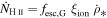${\dot{N}}_{{\rm{H}}{\rm{II}}}={f}_{\mathrm{esc},{\rm{G}}}\,{\xi }_{\mathrm{ion}}\,{\dot{\rho }}_{* }$ , found in our self-consistent modeling compared to that found in those studies (see Figure 6). As we will show in Section 5.3, that increased ${\xi }_{\mathrm{ion}}$ value is due to a notably larger (by a factor ∼2) contribution of low-mass galaxies with much lower metallicities (more than one order of magnitude lower than near solar).

Figure 6. Refer to the following caption and surrounding text. — **Figure 6.** Effective LyC photon production rates predicted in models S and D for galaxies with any mass and metallicity (solid lines) and for galaxies with stellar masses larger than $\sim 5\times {10}^{9}$ ${M}_{\odot }$ and near solar metallicities only (dashed lines; the predictions from the two models superpose). The dashed line coincides, except for a factor 1.61 due to the different IMF used, with the LyC photon production rate predicted in the reionization models by Robertson et al. (2015), Ishigaki et al. (2015), and Bouwens et al. (2015).
Download figure:
Standard image High-resolution image

**Figure 6.** Effective LyC photon production rates predicted in models S and D for galaxies with any mass and metallicity (solid lines) and for galaxies with stellar masses larger than $\sim 5\times {10}^{9}$ ${M}_{\odot }$ and near solar metallicities only (dashed lines; the predictions from the two models superpose). The dashed line coincides, except for a factor 1.61 due to the different IMF used, with the LyC photon production rate predicted in the reionization models by Robertson et al. (2015), Ishigaki et al. (2015), and Bouwens et al. (2015).
Download figure:
Standard image High-resolution image

5.2. Fits to the Observed Global Properties

In Figure 7 we show the fits to the global data that result in the best models S and D. As it can be seen, both solutions recover satisfactorily the observed evolution of all cosmic properties. The only exception is the STH (panel (b)) and, to a much lesser extent, the CGH (panel (a)). Since the STH is the time-integral of the SFH, and this latter curve is very well fitted (see panel (j)), the poor fit to the STH simply reflects the well-known inconsistency between the data sets of the two cosmic histories. We will come back to this point in Section 5.3. The possible origin of the slight excess in the predicted cold gas mass density at $z\lt 3$ will also be discussed in Section 5.4.

Figure 7. Refer to the following caption and surrounding text. — **Figure 7.** Evolution of galaxies and IGM predicted in models S and D, compared to the observational data shown in Figure 1. We plot the contribution from normal galaxies (solid lines) and normal galaxies plus Pop III star clusters (dotted lines); in panel (k) we also plot the contribution of AGNs (dashed lines). In panels (d), (e), and (f), we plot the average metallicities in halos and galaxies within the mass ranges covered by the data (thin solid lines), as well as the average metallicities over all halos and galaxies (thick solid lines) with no corresponding data. In panels (h) and (i) predictions are only shown at the redshifts where galaxies with masses around 10¹¹ ${M}_{\odot }$ are abundant enough. In panel (l) we show the average IGM temperatures in singly ionized (solid lines), doubly ionized (dashed lines), and neutral (dotted lines) regions, the latter shifted a factor 500 upward at z higher than the redshift of first (or unique) complete ionization. Note that the sum at any z of the densities in the left-hand panels gives the total baryon mass density at that z (scaled to the constant critical density at z = 0), and the sum at any z of the product of the metallicities in the middle panels times the corresponding densities in the left panels gives the cumulative mass density of metals produced until that z.
Download figure:
Standard image High-resolution image

**Figure 7.** Evolution of galaxies and IGM predicted in models S and D, compared to the observational data shown in Figure 1. We plot the contribution from normal galaxies (solid lines) and normal galaxies plus Pop III star clusters (dotted lines); in panel (k) we also plot the contribution of AGNs (dashed lines). In panels (d), (e), and (f), we plot the average metallicities in halos and galaxies within the mass ranges covered by the data (thin solid lines), as well as the average metallicities over all halos and galaxies (thick solid lines) with no corresponding data. In panels (h) and (i) predictions are only shown at the redshifts where galaxies with masses around 10¹¹ ${M}_{\odot }$ are abundant enough. In panel (l) we show the average IGM temperatures in singly ionized (solid lines), doubly ionized (dashed lines), and neutral (dotted lines) regions, the latter shifted a factor 500 upward at z higher than the redshift of first (or unique) complete ionization. Note that the sum at any z of the densities in the left-hand panels gives the total baryon mass density at that z (scaled to the constant critical density at z = 0), and the sum at any z of the product of the metallicities in the middle panels times the corresponding densities in the left panels gives the cumulative mass density of metals produced until that z.
Download figure:
Standard image High-resolution image

The fits to the data are particularly good in the case of model D. The predicted SFH almost fully matches the data, while in model S it only does so marginally (see panel (j)). This is reflected in the respective ${\chi }^{2}$ values of 1.07 and 2.65.²⁸ Likewise, the predicted CGH in model D is almost as shallow as the observed curve in the redshift range covered by the data, while that in model S is slightly steeper (see panel (b)); the respective ${\chi }^{2}$ values are 1.90 and 2.35. The predicted HGMH, CGMH, and STMH curves for the metallicities averaged over all halos and galaxies are also substantially different in the two models. However, when the averages are restricted to the mass ranges included in the observations, the two models agree with the data (see panels (e)–(f)). Similarly, the predicted GAMH and GASH are somewhat different at high-z in the two models, but they both match the data at $z\sim 2\mbox{--}3$ (see panels (h) and (i)). Last, the predicted IGMMH is larger in model D than in model S (see panel (g)). However, the empirical bounds on this quantity are not very reliable (see below). A full comprehensive picture of the interconnected behavior of all these cosmic histories will be given in Sections 5.3 and 5.4.

And what about the observational constraints on reionization? In Table 3 we give the values predicted in the best models S and D. The error bars mark those predicted in the models bracketing the two sets of acceptable solutions around them. The values of ${z}_{\mathrm{ion},{\rm{H}}}$ and ${d}_{z}{Q}_{{\rm{H}}{\rm{II}}}$ satisfy, of course, the observed constraints because they have been enforced as priors. But the values of $\tau$ and y are checked for the first time. The values of the Compton distortion y-parameter predicted in models S and D pass the test without trouble: they are one order of magnitude lower than the observed upper limit. The predicted values of $\tau$ are also consistent with the empirical estimates drawn from the WMAP9 and Planck3 data at the $1\sigma$ level. However, while the value predicted in model S still agrees at the 1σ level with the estimate of 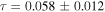$\tau =0.058\pm 0.012$ recently reported by the Planck team, that in model D only does at the 3σ level. We remind the reader that the way the condition ${d}_{z}{Q}_{{\rm{H}}{\rm{II}}}(z=7)\lt 0$ was enforced in this model warrants that the redshift of first complete reionization is as small as possible, so the only way to further decrease the predicted value of $\tau$ is to relax that condition. This possibility cannot be discarded, indeed: the typical outflow velocity of gas clouds in LAEs could decrease with increasing z so that the absence of LAEs at $z\gt 7$ would not imply that ${Q}_{{\rm{H}}{\rm{II}}}(z)$ is decreasing at z = 7.²⁹ In any event, there is also the caveat that the value of $\tau$ inferred from the CMB anisotropies under the instantaneous reionization approximation is quite uncertain.

Table 3. Reionization Constraints

Model	${z}_{\mathrm{ion},{\rm{H}}}$	${d}_{z}{Q}_{{\rm{H}}{\rm{II}}}(z=7)$	$\tau$	$y\times {10}^{5}$
	${6.0}_{-0.5}^{+0.3}$	$\lt 0$	$0.084\pm 0.017$ ^a	$\lt 5$
S	${6.0}_{-0.5}^{+0.3}$	$-{0.19}_{-0.02}^{+0.02}$	${0.072}_{-0.005}^{+0.004}$	0.25 ± 0.01
D	${6.0}_{-0.5}^{+0.3}$	$-{0.13}_{-0.02}^{+0.03}$	${0.102}_{-0.001}^{+0.001}$	0.26 ± 0.01

Note.

^aThis empirical value of $\tau$ combines those inferred from the WMAP nine-year and the Planck three-year data.

Download table as: ASCII Typeset image

5.3. Checking the Differential Properties

But the fact that models S and D fit all the observed global properties, in particular the SFH and MBHH, does not necessarily mean that they also recover the observed galaxy stellar or MBH MFs. In the present section we check that, describing in detail the formation and properties of galaxies and MBHs of different masses.

At high-z halos are barely massive and their concentration is high, so the hot gas cools very efficiently. But, for this to happen, halos must first trap gas, that is, their virial temperature must be higher than the IGM temperature, ${T}_{\mathrm{IGM}}$ . The minimum mass of halos trapping gas at z is

where we have taken into account that the inner mean density of halos at z is a factor ${\rm{\Delta }}(z)$ (close to 178 at high-z) times the mean cosmic density $\bar{\rho }(z)$ . Therefore, new luminous objects (Pop III star clusters or galaxies) will form as long as new halos will trap gas (with undercritical or overcritical metallicity, respectively), that is, as long as ${M}_{\mathrm{trap}}(z)$ will decrease or increase less rapidly than the always increasing typical halo mass of collapse at z, ${M}_{{\rm{c}}}(z)$ , equal to the mass for which the rms density perturbation equals the critical overdensity for ellipsoidal collapse at z (e.g., Juan et al. 2014b). ${M}_{{\rm{c}}}(z)$ is fully determined by cosmology, so the formation of new luminous objects depends only on the evolution of ${T}_{\mathrm{IGM}}(z)$ .

The temperature of the neutral cosmic gas decouples from the CMB temperature at $z\sim 150$ , when Compton heating of residual electrons from CMB photons becomes negligible. Then, the cosmic neutral gas cools adiabatically as ${(1+z)}^{2}$ until the first Pop III stars form. The X-ray background they produce (mostly through PISNe explosions) heats the neutral regions above the CMB temperature by Compton scattering from the diffuse residual electrons. However, Compton cooling from CMB photons prevents such a heating from being too marked, and ${T}_{\mathrm{IGM}}(z)$ diminishes essentially as $1+z$ until Compton cooling progressively declines by the dilution of CMB photons. Then, the temperature of neutral regions keeps on diminishing almost as ${(1+z)}^{2}$ as X-ray heating is insufficient to balance adiabatic cooling (see Figure 7, panel (l)).

Such an evolution of ${T}_{\mathrm{IGM}}(z)$ in neutral pristine regions implies that ${M}_{\mathrm{trap}}(z)$ decreases roughly as ${(1+z)}^{3/2}$ all the time except for a short intermediate period where it is kept essentially constant. Meanwhile, ${M}_{{\rm{c}}}(z)$ starts growing very rapidly, and progressively slows down from ${(1+z)}^{-2}$ above z = 20 to ${(1+z)}^{-1}$ below z = 6, being proportional to ${(1+z)}^{-3/2}$ at an intermediate redshift of about 10. As a consequence, Pop III star clusters are permanently forming in neutral pristine regions. The situation is different, however, in the neutral polluted nodes that develop in model D during recombination. There, the temperature is kept much more constant (see Figure 7, panel (l)),³⁰ causing ${M}_{\mathrm{trap}}(z)$ to increase roughly as ${(1+z)}^{-3/2}$ , that is, more rapidly than ${M}_{{\rm{c}}}(z)$ since $z\sim 10$ . Consequently, no Pop III stars will form in this model after that redshift.

More specifically, ${M}_{{\rm{c}}}(z)$ starts from a very tiny value, and does not reach what is believed to be the neutralino free streaming mass, 10⁻⁶ ${M}_{\odot }$ , until $z\sim 23$ . This means that the only halos present at any higher redshift (necessarily more massive than the free streaming mass of DM particles) are much more massive than the typical collapse mass at that z. Thus their abundance is insignificant. In fact, the first mini-halo (of $\sim 5\times {10}^{5}$ ${M}_{\odot }$ ) able to trap gas and form a Pop III star cluster (of ∼2000 ${M}_{\odot }$ ) within the current horizon is found at $z\sim 48$ .

As the temperature of the neutral IGM decreases, the mass of mini-halos able to form Pop III star clusters diminishes, and, at z∼45, it is low enough for such halos to lose their metal-enriched gas into ionized bubbles when the most massive Pop III stars explode in PISNe. Then the IGM metallicity in ionized regions rapidly increases above ${Z}_{{\rm{c}}}$ . From that moment, when the ionized metal-enriched gas is trapped by halos, it rapidly undergoes atomic cooling, and gives rise to the formation of normal galaxies. But the IGM in ionized bubbles is also photo-heated to a much higher temperature than in neutral regions, so halos able to trap ionized gas are again very massive and rare. In fact, at those redshifts most galaxies form instead in slightly less massive halos (of $\gtrsim {10}^{6}\mbox{--}{10}^{7}$ ${M}_{\odot }$ ) that retained part of the hot gas when Pop III stars exploded. Since the amount of gas remaining in such halos can be very small, most of those galaxies are “failed” in the sense that they have very low stellar masses (from 10² ${M}_{\odot }$ to 10⁵ ${M}_{\odot }$ ).

As halos able to trap fresh metal-enriched ionized gas become increasingly abundant, more and more galaxies form with stellar masses above 10⁵ ${M}_{\odot }$ . This leads to the development of a bimodal MF. But the formation of normal galaxies causes ionized regions to be photo-heated to an approximately constant temperature, so ${M}_{\mathrm{trap}}(z)$ finally increases at the same rate, ${(1+z)}^{-3/2}$ , as ${M}_{{\rm{c}}}(z)$ at $z\sim 10$ . Consequently, the formation of new galaxies with stellar masses above $\sim {10}^{6}$ ${M}_{\odot }$ (the lower mass limit is slowly increasing with decreasing z) is halted roughly at that redshift.

From that moment, the evolution of luminous sources differs in the two models. In model S, Pop III star clusters keep on forming in neutral pristine regions, and galaxies keep on growing, although not forming, in ionized ones. While, in model D, Pop III stars stop forming at $z\sim 10$ when the first complete reionization takes place. (Remember that no Pop III stars form in the neutral polluted regions that develop during the subsequent recombination period.) There is thus a sudden lack of ionizing photons that could definitely interrupt the reionization process. Fortunately, recombination yields a big dip in the IGM temperature of ionized regions (see Figure 7, panel (l)) that allows halos with masses as small as 10⁸ ${M}_{\odot }$ to trap fresh ionized gas. As explained next, the metallicity of this gas is still overcritical, so an abundant amount of normal galaxies then form that partially replace Pop III stars in the production of ionizing photons. This will allow reionization to recover by $z\sim 7.2$ .

Indeed, the IGM metallicity in ionized regions is initially kept roughly constant due to the fixed proportion of metals ( $\propto {f}_{2}$ ) and ionizing photons ( $\propto {f}_{2}+{f}_{3}$ ) provided by Pop III stars. But, once normal galaxies begin to form, there is a larger contribution of ionizing photons than of metals (remember that metals ejected from galaxies mainly stay within halos), so the metallicity of ionized regions begins to decrease. This does not prevent, of course, the total average IGM metallicity from growing (Figure 7, panel (g)) through the increasing weight of ionized regions. But the metallicity of ionized regions themselves can become undercritical. This is actually what happens in model S where the minimum value of ${f}_{2}/({f}_{2}+{f}_{3})$ just needs to warrant the overcritical metallicity when ionized bubbles form. (The undercritical metallicity of these regions at $z\lt 10$ in model S has no effect in the reionization process because no galaxies can form anyway in this model since $z\sim 10$ .) The situation is different, however, in model D where the IGM temperature decreases since $z\sim 10$ . Provided the minimum value of ${f}_{2}/({f}_{2}+{f}_{3})$ is large enough (the maximum value of ${M}_{\mathrm{III}}^{\mathrm{up}}$ low enough) to warrant that the IGM metallicity in ionized regions is still overcritical at $z\sim 10$ , new galaxies will form, indeed, in this model from that redshift to about $z\sim 7$ when the temperature of the ionized IGM increases again at a high enough rate for ${M}_{\mathrm{trap}}(z)$ to grow more rapidly than ${M}_{{\rm{c}}}(z)$ .³¹ The minimum mass of trapping halos in model D during that period is the largest ever been, and the metallicity of the initial hot gas is the lowest, so the cooling rate reaches very low values. As a consequence, a large fraction of these second-generation normal galaxies have very small stellar masses, similar to those of the above-mentioned failed galaxies.

Since $z\sim 10$ in model S or since $z\sim 7$ in model D, no new galaxies form. Galaxies just grow at the center of halos through the accretion of new cooled gas and satellite captures. Of course, some of them freeze out as they become satellites of other central galaxies when their host halos are captured by other halos. Consequently, at any z lower than 7, there are in both models galaxies with the whole spectrum of stellar masses. The only difference is that, while in model S all the very low-mass satellites are failed galaxies, in model D many of them are second-generation galaxies formed at z < 10. Notice that, even though halos where those two kinds of galaxies form have similar masses, ${M}_{{\rm{c}}}(z)$ is much greater at $z\lt 10$ than at the formation of failed galaxies, so those second-generation low-mass galaxies are more abundant than failed ones.

Figure 8 shows the galaxy stellar MFs that result in models S and D at redshifts z = 3.8 and z = 6.8. To compare them with the empirical MFs inferred by González et al. (2011) at the same redshifts we need to account for the above-mentioned inconsistency between the SFH and STH data sets. Indeed, at high- and low-z, the predicted STH curve, consistent with the empirical SFH one, is close to the upper envelope of the stellar mass density estimates, and between $z\lesssim 6$ and $z\sim 4$ it is even higher (see Figure 9). Wilkins et al. (2008) put forward that such an inconsistency could be due to a z-varying IMF. However, the largest discrepancy is found at an intermediate redshift range, which would require the IMF to have a strange non-monotonous trend. A simpler explanation is that the correction for dust attenuation achieved in the galaxy UV luminosities is typically underestimated. Galaxies in the redshift range $4\lesssim z\lesssim 6$ would be substantially brighter than believed, the effect being less marked at higher and lower redshifts because of the lower metallicity of galaxies and the more accurate correction achieved, respectively. But, whatever the real cause of that inconsistency, provided all the observed galaxies are similarly affected, the shape of the MFs derived from the UV LFs would be right except for an horizontal shift. Specifically, according to the stellar mass density estimated inferred by González et al. (2011) at redshifts 3.8 and 6.8 and the theoretical STH curve consistent with the empirical SFH one, the MFs used by González et al. (2011) to infer those estimates should be shifted in model D (S) by a factor of about 6.0 (7.9) and 1.3 (0.8), respectively. Taking into account that the extrapolations of those empirical MFs were underestimated by factors of 1.6 (1.3) and 2.1 (1.4), respectively, the actual shifts to be applied at those redshifts are 9.5 (10.3) and 2.7 (1.2), respectively. As can be seen in Figure 9, these shifts make the empirical MFs fully match indeed the predicted ones except for the incomplete low-mass bins (see below). Thus the predicted galaxy stellar MFs are in very good agreement with the observations. The fact that the MF predicted at z = 3.8 also matches the Schechter fit to the original (with no shift) galaxy stellar MF recently derived by Caputi et al. (2015) at $3\leqslant z\leqslant 4$ assuming a constant IMF also gives strong support to the interpretation that the inconsistency between the SFH and STH data sets is due to a deficient correction for dust attenuation. According to our results in model D (S), the UV luminosities of galaxies inferred by González et al. (2011) at z = 3.8 and z = 6.8 would be underestimated by 2.5 (2.7) mag and 1.0 (1.1) mag, respectively.

Figure 8. Refer to the following caption and surrounding text. — **Figure 8.** Galaxy stellar MFs predicted for all galaxies (solid lines) and central galaxies (dashed lines) in model S and model D at two representative redshifts. Dots with error bars give the MFs inferred at those redshifts by González et al. (2011) from galaxy UV LFs, shifted consistently with the stellar mass densities in model D (see text).
Download figure:
Standard image High-resolution image

Figure 9. Refer to the following caption and surrounding text. — **Figure 9.** Same Pop II STHs (thick solid lines) and CGHs (thick dashed lines) as in panels (b) and (a) of Figure 7 but extended down to z = 1. Also shown are the stellar mass densities in disks (thin long-dashed lines) and in spheroids (thin dot-dashed lines). To avoid confusion the cold gas mass density estimates are here plotted as open circles. The stellar mass density estimates obtained by González et al. (2011) from the galaxy stellar MFs shown in Figure 8 are plotted as brown dots.
Download figure:
Standard image High-resolution image

Regarding the behavior at lower masses of the predicted MFs, we find the turnover at ∼3.5 dex from the knee in model S, and at ∼4.5 dex in model D. These results are consistent with the latest UV LFs of galaxies observed at $z\sim 3$ (Alavi et al. 2016; Livermore et al. 2016), which find that the turnover is not yet detected at ∼6.5 mag (or ∼2.6 dex in mass) from the knee. We remark that all previous models of galaxy formation predicted the turnover at just ∼3.5 mag (∼1.4 dex in mass) from the knee (Jaacks et al. 2013; Kuhlen et al. 2013), which is contradicted by these observations. In this sense, our model is the first to predict MFs consistent with the observations. According to it, such LFs should still go ∼2.25 mag or ∼4.75 mag deeper in models S or D, respectively, for the turnover to be finally detected.

Model D also predicts the existence of a second bump at very low masses in the galaxy stellar MFs at z = 3.8 caused by the second-generation low-mass galaxies that become satellites soon after their formation. This bump is far from the current observational limits of the galaxy stellar MFs at those redshifts. However, given the small mass of those satellites, a large fraction of them should still survive at z = 0. In model S, there is no such a bump, although the abundance of very low-mass galaxies is also quite high. Thus a prediction of our model, regardless of the version, is that it should be possible to detect at z = 0 very old satellites with masses between 10² ${M}_{\odot }$ and 10⁶ ${M}_{\odot }$ . We describe next the expected metallicity, morphology, and size of those predicted relics.

The hot gas metallicity increases in parallel to the cold gas and stellar metallicities (see Figure 7, panel (d), (e) and (f)). The only effect that partly balances that increase is the accretion by halos of low-metallicity IGM in ionized regions. That increase is more marked in model S than in model D due to the steeper SFH caused by the larger ${\alpha }_{{\rm{G}}}$ value, and hence, the larger amount of stars that are permanently forming in galaxies. Another more subtle difference between the two models is the small dip in the hot gas metallicity in model D after $z\sim 10$ due to the large amount of fresh gas that is being incorporated by halos during recombination owing to the dip in the temperature of the ionized IGM. This translates, of course, in less marked dips in the CGMH and STMH of model D. The stellar and cold gas metallicities of the second-generation galaxies formed in this model during recombination, similar to those of the primordial failed galaxies formed in both models, are of about $10{Z}_{{\rm{c}}}$ , i.e., significantly lower than average.³² On the contrary, the metallicities of galaxies more massive than $5\times {10}^{9}$ ${M}_{\odot }$ are, of course, larger than average (see also Figure 7, panels (e) and (f)) and show a well-understood behavior with z: at the highest redshift where those galactic masses are assembled, such galaxies are extraordinarily massive, having been formed in the merger of evolved high metallicity galaxies; then the metallicities slowly decrease as the masses become increasingly ordinary and such galaxies form through other channels (including accretion of hot gas with lower metallicity); and, when the masses of the galaxies approach the average galaxy mass at $z\sim 4$ , they begin to increase just as the average metallicities do since $z\sim 6$ .

The morphology of galaxies follows from the following general trends. When a galaxy forms, the gas it collects comes from the very central part of the halo, so it has little angular momentum, and it is pilled up in a spheroid. Consequently, the failed galaxies in models S and D as well as the second-generation low-mass galaxies in model D are spheroids. But, soon after their formation, the morphology of galaxies evolves at the center of halos. At very high-z, when cooling is very efficient, galaxies usually collect large amounts of cold gas that render disks unstable. In addition, halos are small, and galaxy mergers frequent, so whenever disks are stable they are short-lived and never reach large radii. But, as halos grow, cooling becomes less efficient and galaxy mergers less frequent, so disks grow larger and are longer-lived. As a consequence, the fraction of spheroid-dominated galaxies slowly decreases with decreasing z. On the other hand, at any given z, the most massive galaxies tend to be spheroids arising from galaxy mergers of massive objects, while disks preferentially lie in intermediate-mass galaxies. These trends explain the observed fraction of spheroid-dominated objects with masses above $\sim {10}^{11}$ ${M}_{\odot }$ at $z\sim 2\mbox{--}3$ . We remark, however, that about 25% of galaxies at those redshifts are red dead ellipticals with no star formation. These galaxies have been excluded from the results shown in panel (h) of Figure 7, as they would go undetected. Therefore, the real fraction of spheroid-dominated massive galaxies at those redshifts is ∼0.65 rather than ∼0.40.

The size of galaxies increases in parallel to their mass from the beginning. In fact, when they form as spheroids from a gas cloud with small angular momentum, even though the metallicity of the gas is low (about ${Z}_{{\rm{c}}}$ ), they undergo a large dissipative contraction until they reach the density of molecular clouds. This leads to stellar systems with the typical density of globular clusters. The size of more evolved spheroids depends on the amount and metallicity of the gas they collect (see Equation (8)). The result is an evolution of the average equivalent radius (measured as the square root of the mass-weighted squared equivalent radii of the bulge and the disk, if any) of spheroid-dominated galaxies with masses above 10¹¹ ${M}_{\odot }$ that recovers the observations at $z\sim 2\mbox{--}3$ (Figure 7, panel (i)). Specifically, when those very massive galaxies appear for the first time in dry mergers of massive spheroids, their equivalent radius is even slightly larger than that of present-day slightly contracted spheroids of the same mass; this radius begins to decrease as the mass becomes increasingly ordinary and those galaxies form from unstable disks and wet mergers; it then increases again up to a secondary maximum caused by the increasing lack of gas followed by the increase of the gas metallicity at $z\sim 5$ (see Figure 7, panel (e)); and it finally increases until z = 0 due to the definite small amount of gas present in galaxies.

Thus the properties of very low-mass galaxies are essentially the same in both models. They are among the first objects with Pop II stars to form; they are spheroids with no gas; they are very compact, with the typical density of globular clusters; and their Pop II stars have very low metallicities (of about 10–100 times ${Z}_{{\rm{c}}}$ , with ${Z}_{{\rm{c}}}$ equal to $\sim 0.25\times {10}^{-4}$ ${Z}_{\odot }$ in model S, and $\sim {10}^{-4}$ ${Z}_{\odot }$ in model D). On the other hand, those of them that froze out as satellites soon after formation have very large baryon-to-DM mass ratios as their original DM halos are truncated by the potential well of the also quite dense capturing halo near the region where all the stars are strongly concentrated. And the fraction of those satellites that will be captured a long time afterward (because of the slight dynamic friction they suffer) by evolved, much less dense galaxies will survive inside them as small independent dynamical entities.

Clearly, all these properties greatly resemble those of present-day globular clusters. Since such objects are often seen to freely orbit within halos, they should have formed outside galaxies and have a cosmological origin similar to them. It is thus not surprising that a self-consistent model such as AMIGA that monitors the formation and evolution of luminous objects since the dark ages does not miss them. Notice that, if this is indeed the origin of globular clusters, the larger abundance of such objects compared to massive galaxies is more consistent with model D than with model S.

Let us now turn to the MFs of MBHs. MBHs grow since the remnant mini-MBHs of Pop III star clusters begin to develop at the center of galaxies (Figure 7, panel (c)). There, they merge with the MBHs brought by accreted or merged galaxies having reached the center of the galaxy by dynamical friction, and accrete new material. Indeed, when some amount of gas reaches the spheroid it fuels the MBH. The associated AGN is then lit, and begins to reheat the circumnuclear gas, quenching the star formation that is going on in the spheroid. The more massive the MBH, the larger both the AGN bolometric luminosity and the fraction of gas reheated and expelled from the spheroid back into the halo. This leads to a self-regulated growth of MBHs and stellar spheroids, which tends toward a constant MBH-to-spheroid mass ratio as observed (Figure 10). This thus gives strong support to the mechanism proposed by Di Matteo et al. (2005) included in AMIGA for the coupled growth of MBHs and spheroids.

Figure 10. Refer to the following caption and surrounding text. — **Figure 10.** Same MBHHs (thick solid lines) as in panel (c) of Figure 7 but extended down to z = 1. Also shown are the spheroid mass density history (thin dashed lines), and disk mass density history (thin dot-long-dashed lines). Empty circles give the MBH mass density estimates obtained from rough (incomplete and uncorrected for obscuration and inactivity) MBH MFs. Brown dots at z = 3.3 and z = 6.1 correspond to the estimates derived by Kelly et al. (2010) and Willott et al. (2010a), respectively, from the MFs used in Figure 11.
Download figure:
Standard image High-resolution image

The parallel evolution of spheroids and MBHs goes together with that of disks. Of course, when gas replenishment begins to decline by $z\sim 7$ (see Section 5.4), the disk and spheroid mass density histories become slightly shallower. (The change of slope is a little less marked in spheroids than in disks due to their unchanged behavior in major mergers.) But this has a minor effect in the parallel evolution of the spheroid and MBH stellar mass densities because mergers become at the same time increasingly dry. Indeed, in dry mergers spheroids grow through the addition of stars belonging to the merging galaxies, while MBHs grow by coalescence of the respective MBHs and, since the MBH-to-spheroid mass ratio is the same in all the progenitors, it remains unchanged in the final object. As a consequence, the MBH and spheroid mass ratio will be kept essentially unaltered until z = 0.

Figure 11 shows the MBH MFs predicted at redshifts z = 3.3 and 6.1. As in the case of the galaxy stellar MFs, to compare these MFs to the empirical ones derived at the same redshifts by Willott et al. (2010a) and Vestergaard et al. (2008) we must take into account any effect that could affect the latter. As mentioned, the observed AGN LFs are greatly affected by incompleteness, obscuration, and inactivity, which cause the MBH mass density estimates derived from them to be much lower than expected from the observed constant MBH-to-spheroid mass ratio. Incompleteness affects in an uneven way the different mass bins of the MBH MFs, but their large mass end should be complete. Obscuration is also larger for low-mass objects (Ueda et al. 2003), but the most massive bins should be similarly affected. Thus a vertical shift by a factor s₁ of a few hundreds should be enough to correct the empirical MBH MFs for obscuration and inactivity. In addition, there is the uncertainty in the MBH mass estimates themselves coming from the poorly determined virial factor, f_σ or ${f}_{\mathrm{FWHM}}$ . For instance, the MBH masses derived by Willott et al. (2010a) and Vestergaard et al. (2008) at z = 6.1 and 3.3, respectively, from emission-line reverberation assume ${f}_{\mathrm{FWHM}}=1.17$ (Collin et al. 2006), while, according to Yong et al. (2016), this factor could be up to a factor of five smaller. Consequently, the empirical MBH MFs derived by those authors might also need to be shifted horizontally toward large masses by a factor s₂ in the range $1\geqslant {s}_{2}\geqslant 0.2$ . The value of s₂ is unknown, but it should be independent of z. On the other hand, the shifts ${s}_{1}/{s}_{2}$ these effects would cause to the MBH mass density estimates derived by Kelly et al. (2010) and Willott et al. (2010a) should make them match the predicted MBHH curve consistent with the observed MBH-to-spheroid mass ratio, equal to ∼400 and ∼250 at z = 3.3 and z = 6.1, respectively (see Figure 10).³³ Taking into account the different degrees of completion in the extrapolated MFs used in the calculation of those MBH mass density estimates, the vertical shifts to be applied to the corresponding MFs at z = 3.3 and z = 6.1 should be 1.58 and 1.70 times larger, respectively. Therefore, with the only freedom of the z-independent value of s₂ (with $1\geqslant {s}_{2}\geqslant 0.2$ ), it should be possible to shift the empirical MFs at the two redshifts so as to match those predicted at the two redshifts. As shown in Figure 11, this is indeed what we find for s₂ = 0.33 (or ${f}_{\mathrm{FWHM}}=0.39$ ). Notice that, as a consequence of the small correction in ${f}_{\mathrm{FWHM}}$ , the upper mass limit of MBHs at z = 3.3 becomes $\sim {10}^{10}$ ${M}_{\odot }$ , which is more reasonable than the original value of $\sim 3\times {10}^{10}$ ${M}_{\odot }$ if we compare with such an upper limit at z = 0.

Figure 11. Refer to the following caption and surrounding text. — **Figure 11.** MFs of MBH in central galaxies (dashed lines) and in all galaxies (solid lines) predicted in models S and D at two representative redshifts. Dots with error bars give the MBH MFs inferred at those redshifts by Willott et al. (2010a; top panel) and Vestergaard et al. (2008; bottom panel) from optical AGN LFs, shifted consistently with the MBH mass densities in model D and a well-suited ${f}_{\mathrm{FWHM}}$ value (see text).
Download figure:
Standard image High-resolution image

**Figure 11.** MFs of MBH in central galaxies (dashed lines) and in all galaxies (solid lines) predicted in models S and D at two representative redshifts. Dots with error bars give the MBH MFs inferred at those redshifts by Willott et al. (2010a; top panel) and Vestergaard et al. (2008; bottom panel) from optical AGN LFs, shifted consistently with the MBH mass densities in model D and a well-suited ${f}_{\mathrm{FWHM}}$ value (see text).
Download figure:
Standard image High-resolution image

5.4. Reliability of the Model

It might be argued that the model could be wrong and the solutions found for some appropriate values of the free parameters still recover the observed global and differential cosmic properties at $z\gt 2$ . But such good results have been achieved with less than one degree of freedom per curve, which is unbelievable for any model that would not include the right physics. To see this we must simply think, for instance, in the fitting by means of a well-suited function with no physics of one single monotonous curve such as the observed SFH at $z\gt 2$ requires four parameters (e.g., Robertson et al. 2015). Furthermore, not only does our model with only nine degrees of freedom provide very good fits to the dozen observed curves at $z\gt 2$ (plus the galaxy stellar and MBH MFs), but it also automatically recovers all their extreme and saddle points at $z\sim 2$ with no need to change the value of any parameter.

As mentioned, disks become increasingly abundant as z decreases, so the cold gas mass density increases (Figure 7, panel (a)). But cooling becomes increasingly inefficient, and by $z\sim 7$ the rate of gas storage in disks begins to decline and the CGH becomes increasingly shallower. This effect is particularly marked in model D, where the CGH reaches a plateau between $z\sim 5$ to $z\sim 3$ . The observed CGH is also flat at those redshifts, but the plateau reaches $z\sim 2$ (see Figure 7, panel (b)). There are several possible causes for that small discrepancy, such as the fact that the empirical cold gas mass density estimates do not include molecular gas or that observations may be biased toward large (massive) DLAs, which have the lowest gas content. But the most likely reason is that satellite interactions, neglected in the present work, begin to have a significant impact in the amount of gas present in disks. In any event, the predicted stagnation of cold gas around $z\sim 4$ corresponds to a saddle point, not to a maximum, in agreement with observation (e.g., Péroux et al. 2003; Prochaska et al. 2005). At lower redshifts the temperature of the singly and doubly ionized IGM begins to diminish (see Figure 7, panel (l)), causing a rather constant slope in the HGMH, and the continuation of cooling.

Of course, the SFR density of ordinary (Pop II ) stars increases in parallel to the cold gas mass density (see Figure 9), so when gas replenishment begins to decline by $z\sim 7$ , the SFR density also slows down. Until that redshift, spheroids were much more abundant than disks, which never collected large amounts of gas. Nonetheless, disks were small, so their dynamical time was short, and the SFR density in disks was notable (see Figure 12). The small amount of gas in disks also prevents the SFR density in mergers from being too large. It is just comparable to that in unstable disks at high-z, and reaches a maximum at $z\sim 6$ . This does not mean that mergers are less frequent from that moment; they just become increasingly dry. As the cooling rate declines, the SFR in individual unstable disks also does, but the corresponding global SFR density keeps on increasing because of the increasing abundance of spheroids contributing to it. The same happens with disks: even though the size of disks increases and the amount of cold gas they harbor decreases with decreasing z so that the SFR in individual disks decreases, the global SFR density in disks keeps on increasing because of the increasing abundance of disks. As a result, the ratio between the SFR densities in disks and spheroids is kept roughly constant. However, the declining amount of cold gas in disks ultimately causes the SFR in both unstable and stable disks to reach a maximum at $z\sim 2$ , and then to rapidly diminish toward z = 0 (see Figure 12). Therefore, the origin of this maximum in the SFH is the same as for the plateau in the CGH: the lack of gas replenishment. However, in the SFH case, such a stagnation leads to a real maximum, not to a saddle point as in the CGH case. The drop in the SFR in disks and spheroids at $z\sim 2$ is so marked that, even though at lower redshifts the cold gas mass density begins to increase again, the total SFR density will keep on decreasing until z = 0.

Figure 12. Refer to the following caption and surrounding text. — **Figure 12.** Same Pop II SFHs (thick solid lines) as in panel (i) of Figure 7 but extended down to z = 1. Also shown are the contributions from disks (thin solid lines) and spheroids arising from galaxy mergers (thin short-dashed lines) or direct infall of cold gas in unstable disks (thin long-dashed lines).
Download figure:
Standard image High-resolution image

The stagnation of cold gas mass at $z\lesssim 5$ has a similar effect on the SFH in models S and D. But the rest of the curve is slightly different in the two models. In model D, the SFH grows more steeply at high-z despite the smaller value of ${\alpha }_{{\rm{G}}}$ (see Figure 7, panel (j)) because of the more rapid growth of ionized regions where normal galaxies lie. But, near z = 10 the formation of Pop III stars declines and ionized regions stop growing, causing the SFH to become shallower. This yields a concave curvature in the SFH of model D that perfectly fits the data. Instead, the SFH in model S has a more constant slope. This difference in the SFH of both models combined with the large abundance of spheroids with a very efficient SN heating also translates into a larger amount of hot gas in model D between $z\sim 12$ to $z\sim 5$ (see Figure 7, panel (x)). Unfortunately, there are no observational data on this quantity yet, so the behavior of the HGMH in the two models cannot be checked.

The behavior of the IEH from galaxies and AGNs follows from the evolution of those two kinds of sources described above. At very high-z, Pop III stars have the dominant contribution. But this contribution diminishes as neutral pristine regions progressively disappear. In model D it completely vanishes at $z\sim 10$ when Pop III stars stop forming, whereas in model S it continues until z ∼ 6. On the other hand, the maximum contribution from AGNs is one order of magnitude smaller at $z\sim 2$ . Consequently, the H i-ionizing emissivity at $z\lesssim 6$ is always dominated by normal galaxies, and its evolution closely follows the SFH associated with ordinary stars. In particular, the IEH also reaches a maximum at $z\sim 2$ (see Figure 13). What is less obvious is the maximum in both models S and D of the H i- and He ii-ionizing (as well as the X-ray) emissivities from AGNs at that redshift (Figure 13): the MBH mass density is ever increasing at $z\lt 2$ (see Figure 10) so we could naively expect their emissivities to do so also. What causes these maxima is the fact that the most massive MBHs stop being fueled by that redshift (their galaxies undergo dry mergers). Consequently, the bright AGNs stop radiating as quasars, and remain in the more quiescent radio phase. This has a major impact in the global AGN emissivities because bright AGNs have the largest bolometric luminosity (e.g., Hatziminaoglou et al. 2003). However, massive MBHs keep on growing through dry mergers and less massive ones through wet mergers of low-mass galaxies that still harbor gas.

Figure 13. Refer to the following caption and surrounding text. — **Figure 13.** Same IEHs from normal galaxies (solid lines) and AGNs (dashed lines) as in panel (k) of Figure 7 but extended down to z = 1.
Download figure:
Standard image High-resolution image

6. SUMMARY AND DISCUSSION

Observational data on the high-z universe are now numerous and accurate enough to severely constrain the interconnected evolution of galaxies and IGM. In fact, they would completely determine it provided the IGM metallicity and temperature were known at $z\gtrsim 6$ . These pieces of information are needed, indeed, to determine the threshold metallicity ${Z}_{{\rm{c}}}$ for atomic cooling and the Pop III star IMF that play a crucial role in the reionization process. Assuming that IMF is a power law, the conditions that the metallicity of ionized regions must be high enough for triggering sustained galaxy formation and Pop III stars massive enough for seeding MBHs greatly constrain those two properties.

The only acceptable solutions we find are in two narrow sets, one for small ${M}_{\mathrm{III}}^{\mathrm{lo}}$ values (moderately top-heavy Pop III star IMFs) leading to single reionization, and another one for large ${M}_{\mathrm{III}}^{\mathrm{lo}}$ values (top-heavier Pop III star IMFs) leading to double reionization. The latter solutions have a first ionization phase driven by Pop III stars completed at $z\sim 10$ , and after a short recombination period a second ionization phase driven by normal galaxies completed at $z\sim 6$ . In the former solutions with single reionization, both kinds of luminous sources contribute in parallel to the ionization of the IGM, completed at $z\sim 6$ .

The best solution with double reionization gives excellent fits to all the observables. Instead, the best solution with single reionization predicts a too-monotonous SFH, and a slightly too steep CGH at z ∼ 4. However, the CMB Thomson optical depth found in double reionization ( $\tau ={0.102}_{-0.001}^{+0.001}$ ), though consistent with the observational estimates from the WMAP 9-year and Planck three-year data, is $3\sigma$ larger than the most recent estimate ( $\tau =0.058\pm 0.014$ ) from the Planck data taking into account the large-scale polarization anisotropies. Instead, the CMB optical depth found in single reionization ( $\tau ={0.072}_{-0.005}^{+0.004}$ ) is consistent with that estimate. There is thus some tension between the new estimate of $\tau$ and the observed properties of the universe at high-z. However, the empirical values of the CMB optical depth derived under the instantaneous reionization approximation must be taken with caution.

The fact that with only nine degrees of freedom it is possible to fit a dozen independent cosmic histories with non-trivial features (extreme and saddle points) confers strong reliability to our self-consistent model of the EoR.

As a byproduct, we have clarified the origin of some interesting features shown by the data on the high-z universe: (1) the very small sizes of spheroids at $z\sim 2\mbox{--}3;$ (2) the sudden drop of the SFH at $z\lt 2;$ (3) the similar behavior of the UV (and X-ray) emissivity from AGNs at the same redshift; (4) the plateau in the CGH between at $1\lt z\lt 5;$ and (5) the rough constancy of the MBH-to-spheroid mass ratio. Our results also suggest that globular clusters are but the relics of the lowest mass galaxies with primordial origin or, more probably, formed during recombination in model D, which soon become frozen as satellite galaxies.

Finally, we have provided several predictions that should allow one to confirm the validity of the present model and to tell between single and double reionization. The most interesting one is that, in the case of double reionization, LAEs should be detectable near z = 10. This could explain the recent detection (to be confirmed) of a galaxy with Lyα emission at z = 8.68 (Zitrin et al. 2015).

Funding for this work was provided by the Spanish MINECO under projects AYA2012-39168-C03-1, AYA2012-39168-C03-2, AYA2013-446724-P, MDM-2014-0369 of ICCUB (Unidad de Excelencia “María de Maeztu”), AYA2015-70498-C02-2-R (co-funded with FEDER funds), and the Catalan DEC grant 2014SGR86. J.M.M.H. was supported by Spanish MINECO grant ESP2014-59789-P.

Footnotes

7
Compton scattering by CMB photons also heats the neutral phase until $z\sim 150$ , when recombination is no more efficient, and the ionized fraction freezes out.
8
For H i-ionizing photons, we include recombinations to He ii and He iground states. The contribution from He ii Lyα recombinations is neglected for simplicity.
9
Neglecting nonlinear effects (IGM is in linear and mildly nonlinear regimes), the volume average of the heating/cooling by gravitational compression/expansion of density fluctuations vanishes.
10
The exact value depends slightly on z as the temperature of the gas cloud is bounded by the CMB temperature.
11
If ${\beta }_{\mathrm{III}}$ times the mass of the star cluster is less than 260 ${M}_{\odot }$ , whether or not there is a mini-MBH of this latter mass is decided randomly using the Pop III star IMF (see Section 4).
12
Schaerer (2002) presumes the Pop III star IMF with the usual Salpeter slope. But the results are not very sensitive to this assumption because the radiation emitted by all massive Pop III stars has essentially the same spectral energy distribution (SED), equal to that of a blackbody of $\sim {10}^{5}$ K.
13
Caution with the notation used in the present paper for the effective radius of a galaxy component. It coincides with that used in (Manrique & Salvador-Solé 2015) for its length scale.
14
The most massive ellipticals have formed through dry major mergers, and spheroids with low enough mass reach the maximum density of molecular clouds.
15
For instance, the escape fractions from galaxies and AGNs could vary with z. However, neither from a theoretical nor from an observational point of view is that dependence clear. Thus we assume them with fixed typical values, as usual.
16
In all of them the clumping factor and the IMF of ordinary stars are also fixed, as well as the uncertain z-dependent dust attenuation.
17
The STH is the time-integral of the SFH, but the two observables are inferred independently. In fact, as we will see, they turn out to be inconsistent with each other.
18
Given the asymptotic logarithmic slopes of those MFs or LFs, such extrapolations are not expected to have any dramatic effect (but see Section 5.3).
19
Other quantities, such as the metallicity or the time elapsed since the last starburst, are usually varied within reasonable ranges and typical (or favorite) values are adopted.
20
Only about 20%–30% of all AGN are believed to be Compton thick, and hence lost in X-rays (Castelló-Mor et al. 2013). On the other hand, most of them are active at $z\gtrsim 6$ (Willott et al. 2010a) due to the high frequency of unstable disks (see Section 5).
21
Observations show that the MBH-to-spheroid mass ratio is constant at least up to $z\sim 2$ . The mild evolution seen beyond that redshift is likely due to the Malmquist bias (Kormendy & Ho 2013).
22
We adopt the upper envelope because it is more consistent with the SFR density estimates of item (j).
23
Cooling is much more sensitive to the density of the hot gas than to its metallicity, dependent on ${h}_{\mathrm{mix}}$ .
24
The gas mass fueling the MBH is negligible compared to the mass converted into stars.
25
The rationale for a top-heavier Pop III IMF is that the fragmentation of protostellar clouds is favored by metals, absent in the pristine gas.
26
The upper mass of Pop I and II stars is poorly determined. An upper limit of 150 ${M}_{\odot }$ is sometimes considered, although no stars more massive than 130 ${M}_{\odot }$ have ever been observed (Figer 2005; but see Crowther et al. 2010).
27
This is the reason why in most studies dealing with the Pop III star IMF the value of 2.35 is adopted (e.g., Schaerer 2002).
28
All ${\chi }^{2}$ values correspond to the logarithmic curves as plotted in Figure 7 and consider only points with well-measured errors bars (upper and lower bounds are excluded).
29
It could be increasing, and the outflow velocity could be decreasing rapidly enough to balance that increase.
30
This feature should allow one to tell the difference between single and double reionization by looking at the IGMTH. Although there is no temperature estimates at $z\gt 6$ , the spin temperature of hydrogen atoms is already coupled the neutral gas temperature through the Wouthuysen–Field effect, so such a difference between models S and D should leave an unequivocal signal in 21 cm line observations.
31
In fact, since the maximum possible value of ${M}_{\mathrm{III}}^{\mathrm{up}}$ is close to the lower limit of 260 ${M}_{\odot }$ , the average IGM metallicity at $z\sim 10$ cannot be much larger than ${Z}_{{\rm{c}}}$ either (see Figure 7, panel(g)). Therefore, another characteristic of double reionization is that the IGM metallicity at $7\lesssim z\lesssim 10$ is close to ${Z}_{{\rm{c}}}$ .
32
These metallicities are nonetheless larger than the metallicity of the initial gas due to the rapid increase in the metallicity of the gas produced during star formation.
33
These values essentially hold for both models D and S.

Please wait… references are loading.

CONSTRAINING THE EPOCH OF REIONIZATION FROM THE OBSERVED PROPERTIES OF THE HIGH-z UNIVERSE

Article metrics

Permissions

Share this article

Dates

ABSTRACT

1. INTRODUCTION

2. THE MODEL

2.1. IGM

2.2. Luminous Sources

2.3. Parameters

3. THE OBSERVED HIGH-Z UNIVERSE

4. FITTING STRATEGY

4.1. Additional Constraints on the Pop III Star IMF

5. RESULTS

5.1. Reionization History

5.2. Fits to the Observed Global Properties

5.3. Checking the Differential Properties

5.4. Reliability of the Model

6. SUMMARY AND DISCUSSION

Footnotes