Abstract
“Changing-look” quasars are a new class of highly variable active galactic nuclei that have changed their spectral type over surprisingly short timescales of just a few years. The origin of this phenomenon is debated, but is likely to reflect some change in the accretion flow. To investigate the disk–corona systems in these objects, we measure optical/UV–X-ray spectral indices ( ) and Eddington ratios (
 ) of 10 previously discovered changing-look quasars at two or more epochs. By comparing these data with simulated results based on the behavior of X-ray binaries, we find possible similarities in spectral indices below the 1% Eddington ratio. We further investigate the Eddington ratios of changing-look quasars before and after their spectral type changes, and find that changing-look quasars cross the 1% Eddington ratio boundary when their broad emission lines disappear/emerge. This is consistent with the disk-wind model as the origin of broad emission lines.
1. Introduction
Nearly all massive galaxies are believed to host supermassive black holes (SMBHs) at their centers, and those whose SMBHs are actively accreting are observed as active galactic nuclei (AGN). Emissions from nuclear regions of AGN are often time-variable (e.g., Sesar et al. 2007), and some AGN display extreme changes in their broad Balmer emission lines and continuum fluxes in repeat optical spectroscopy (i.e., they change from Type 1 to Type 1.9 when their broad  emission lines disappear, or from Type 1.9 to Type 2 when their broad
  emission lines disappear). These AGN displaying extreme spectral variability have been referred to as changing-look AGN
11
(Collin-Souffrin et al. 1973; Tohline & Osterbrock 1976). Apart from AGN in the local universe, the “changing-look” phenomenon has also been observed in their more luminous and more distant counterparts—quasars. The first changing-look quasar (CLQ) was identified in 2015 (LaMassa et al. 2015). Since then, dozens of CLQs have been discovered in observations from the Sloan Digital Sky Survey (SDSS; see MacLeod et al. 2016; Ruan et al. 2016; Runnoe et al. 2016; MacLeod et al. 2019), the intermediate Palomar Transient Factory (e.g., Gezari et al. 2017), and the Zwicky Transient Facility (e.g., Frederick et al. 2019), or have been identified based on a mid-infrared color transition from a quasar-like color into a galaxy-like color or vice versa (Sheng et al. 2020). Several high-redshift (z > 2) CLQs have also been discovered (Ross et al. 2020). Nevertheless, the physical origin of the CLQ phenomenon is still unclear. Recent observations have suggested that CLQs may be triggered by accretion state transitions (e.g., Noda & Done 2018), possibly analogous to those observed in X-ray binaries. However, the expected transition timescale (∼105 yr) for these state transitions in SMBHs, when directly scaled with the black hole mass (Sobolewska et al. 2011), appears to be incompatible with the short timescales of spectral changes in CLQs (∼5–10 yr). Thus, it is worthwhile to investigate whether there are indeed observable similarities between CLQs and X-ray binaries undergoing accretion state transitions.
emission lines disappear). These AGN displaying extreme spectral variability have been referred to as changing-look AGN
11
(Collin-Souffrin et al. 1973; Tohline & Osterbrock 1976). Apart from AGN in the local universe, the “changing-look” phenomenon has also been observed in their more luminous and more distant counterparts—quasars. The first changing-look quasar (CLQ) was identified in 2015 (LaMassa et al. 2015). Since then, dozens of CLQs have been discovered in observations from the Sloan Digital Sky Survey (SDSS; see MacLeod et al. 2016; Ruan et al. 2016; Runnoe et al. 2016; MacLeod et al. 2019), the intermediate Palomar Transient Factory (e.g., Gezari et al. 2017), and the Zwicky Transient Facility (e.g., Frederick et al. 2019), or have been identified based on a mid-infrared color transition from a quasar-like color into a galaxy-like color or vice versa (Sheng et al. 2020). Several high-redshift (z > 2) CLQs have also been discovered (Ross et al. 2020). Nevertheless, the physical origin of the CLQ phenomenon is still unclear. Recent observations have suggested that CLQs may be triggered by accretion state transitions (e.g., Noda & Done 2018), possibly analogous to those observed in X-ray binaries. However, the expected transition timescale (∼105 yr) for these state transitions in SMBHs, when directly scaled with the black hole mass (Sobolewska et al. 2011), appears to be incompatible with the short timescales of spectral changes in CLQs (∼5–10 yr). Thus, it is worthwhile to investigate whether there are indeed observable similarities between CLQs and X-ray binaries undergoing accretion state transitions.
Accretion state transitions have been detected in many Galactic X-ray binaries (e.g., Maccarone 2003; Debnath et al. 2010; Tang et al. 2011; Wang et al. 2018; Kara et al. 2019). Both black hole and neutron star X-ray binaries show spectral state transitions at ∼1% bolometric Eddington ratios ( ). In these different states, X-ray binaries display distinct X-ray behavior in the hardness-intensity diagram (HID). At high Eddington ratios, their X-ray spectra are dominated by thermal soft X-rays, believed to be emitted from a standard thin accretion disk (Shakura & Sunyaev 1973). When Eddington ratios drop below 1%, the inner parts of the accretion disk may evaporate, causing the spectra to be dominated instead by hard X-rays from either a corona (Frank et al. 1987), an advection dominated accretion flow (ADAF; Narayan & Yi 1995), or a newly launched jet (Markoff et al. 2001). The spectral state associated with high Eddington ratios is called the “High/Soft” state, while the one at lower Eddington ratios is referred to as the “Low/Hard” state. Similar transitions also likely occur in AGN, but due to the expected long transition scales of 105 yr (Sobolewska et al. 2011), we may not expect to directly witness such a transition in AGN. However, by observing the spectral energy distribution (SED) shapes of AGN at different Eddington ratios, and comparing these with the spectral shapes of a single black hole X-ray binary undergoing accretion state transitions, we may be able to better understand and characterize any similarities between supermassive black holes and stellar mass black holes (Ruan et al. 2019a).
By assuming that supermassive black holes have analogous accretion flow structures as those in X-ray binaries, and scaling the disk and the corona emission with black hole mass, Sobolewska et al. (2011) simulate optical/UV–X-ray spectral indices ( ) and bolometric Eddington ratios (
 ) of AGN populations. That work predicts that AGN may display distinct spectral states similar to those observed in X-ray binaries. They predict that at
  ,
,  and
and  show a positive correlation, but this becomes an inverse correlation when
  drops below 1%.
Previous observations of bright quasars often show that there is indeed a positive correlation between their single-epoch  and
and  at
at  (Maoz 2007; Grupe et al. 2010; Lusso et al. 2010). However, for low-luminosity AGN (LLAGN), it is difficult to measure their black hole masses (and thus Eddington ratios), due to the difficulty of detecting broad emission lines in the spectra. A few studies based on LLAGN show a weak negative correlation between their
  and
and  (Maoz 2007; Xu 2011), but additional observations are needed to probe the relation between
  and
and  at
at  . CLQs offer a unique opportunity to probe this relation at
  , by combining black hole masses measured from bright state spectra of CLQs with broad Balmer emission lines present, and
  when CLQs fade. Given that the Eddington ratios of LLAGN are usually much lower than 1% (Gu & Cao 2009; Xu 2011), CLQs are especially helpful to study this
  relation just below 1%
  . By measuring the
  and
and  of six “turn-off” CLQs, Ruan et al. (2019a) find a negative correlation between
  and
and  at
at  , as observed in X-ray binaries. This supports the notion that emission mechanisms from X-ray binaries can be directly scaled to AGN with supermassive black holes. In this work, we report optical and X-ray observations of another 10 CLQs, and test whether a similar relation is borne out by these systems at
  .
.
Dramatic changes in the optical broad emission lines (BELs) of CLQs can also probe the physical origin of the lines themselves. Optical spectra of AGN are characterized primarily by a power-law continuum, BELs, and narrow emission lines (e.g., Vanden Berk et al. 2001). BELs are emitted from the broad-line region (BLR), which is believed to be the high velocity gas gravitationally bound to the central supermassive black hole (Peterson & Wandel 2000; Peterson et al. 2004). Results from reverberation mapping (Denney et al. 2009; De Rosa et al. 2018), and study of the quasar orientation and observed width of BEL profiles (Shen & Ho 2014; Storchi-Bergmann et al. 2017) imply that the geometry of the BLR is likely to be disk-like. Furthermore, study of BEL profiles suggests the BLR gas is structured as a smooth continuous flow (Laor et al. 2006). However, the exact origin of the BLR gas is still unclear (Elvis 2017). The disk-wind model suggests that the BLR gas comes from winds produced by the accretion disk (Emmering et al. 1992; Murray et al. 1995; Murray & Chiang 1997; Elitzur & Ho 2009; Elitzur et al. 2014; Elitzur & Netzer 2016). When the mass accretion rate drops below a certain limit (corresponding to a luminosity of ∼ , where
  is the black hole mass in
  ), winds can no longer be sustained, such that the observed BELs “disappear” (Elitzur & Ho 2009). Below the critical luminosity, AGN are expected to be “true” Type 2 AGN (i.e., Type 2 AGN intrinsically absent of BLRs). Although this critical luminosity is dependent on the black hole mass, the disk-wind model predicts that more detections of BEL disappearance are expected below the 1% Eddington ratio (Elitzur & Netzer 2016), and a double-peaked BEL profile, the signature of a rotating disk, should emerge in the quasar spectrum when the accretion rate drops (Elitzur et al. 2014). Single-epoch observations show that Eddington ratios of bright quasars with prominent BELs, are always higher than 1% (Kollmeier et al. 2006; Steinhardt & Elvis 2010). Yet it is still unknown whether Eddington ratios of individual quasars varying around 1% will display the appearance/disappearance of broad emission lines. By studying the Eddington ratios of the single changing-look AGN UGC 3223, Wang et al. (2020) find this object crosses the 1% Eddington ratio when its AGN type changes. However, it is still necessary to investigate whether this 1% Eddington ratio is associated with appearance/disappearance of BELs with multiepoch observations of CLQs, and with a larger data set. In this work, we also study the changes in the Eddington ratio distributions from the brightest to the faintest optical spectra of CLQs, investigate the possible connection with the 1% Eddington ratio, and study the BEL profiles of those CLQs.
We present optical and X-ray observations of 10 CLQs identified via repeat SDSS photometry and follow-up optical spectroscopy (MacLeod et al. 2016, 2019). We obtain new optical data from the Multiple Mirror Telescope, the Magellan Telescope, the Apache Point Observatory Astrophysical Research Consortium 3.5 m, and the Hobby–Eberly Telescope. We also obtain new X-ray data from the Chandra X-ray Observatory, along with archival data from the XMM-Newton and the ROSAT. This paper is organized as follows: we present our optical data reduction procedures in Section 2, X-ray measurements in Section 3, results and discussion in Section 4, and a brief conclusion in Section 5. Throughout this paper, we adopt the cosmological parameters  ,
,  ,
,  (Bennett et al. 2014).
2. Optical Data Reduction
2.1. Targets and Data
The 10 CLQs studied here were selected from SDSS (York et al. 2000; Abazajian et al. 2009) based on their large amplitude photometric changes, and then confirmed by follow-up optical spectroscopy (MacLeod et al. 2016, 2019). We also obtain new optical spectroscopy from several different telescopes, which we briefly summarize below.
2.1.1. MMT and Magellan
We observe three CLQs with the Blue Channel Spectrograph on the 6.5 m Multiple Mirror Telescope (MMT) during 2016 to 2018 (Angel et al. 1979), with the  grating, covering the wavelength range of 3300–8500 Å at a spectral resolution
12
of 6.47 Å. We use pydis
13
to reduce the MMT data, and calibrate the flux of the observed spectra using a standard star observed on the same night.
grating, covering the wavelength range of 3300–8500 Å at a spectral resolution
12
of 6.47 Å. We use pydis
13
to reduce the MMT data, and calibrate the flux of the observed spectra using a standard star observed on the same night.
We also acquire two spectra from the 6.5 m Magellan Clay telescope, with the Low Dispersion Survey Spectrograph 3 (LDSS3)-C spectrograph. We use the VPH-All grism, which covers the wavelength range of 4250–10000 Å, with a spectral resolving power
14
 . We use both pydis and IRAF, and follow the data reduction procedures in MacLeod et al. (2019) to reduce the data, and perform wavelength and flux calibration.
2.1.2. ARC 3.5 m
For the five Astrophysical Research Consortium (ARC) 3.5-meter telescope observations, we use the Dual Imaging Spectrograph (DIS) with the B400/R300 grating for each spectrum, along with spectra of HeNeAr lamps to perform wavelength calibration. Those spectra cover 3400–9200 Å at a spectral resolving power of R ∼ 1000, with a 15 slit. Spectra of standard stars from the same night are used for flux calibration. We use IRAF to perform bias and flat-field corrections, aperture extraction, and wavelength and flux calibration (Tody 1986, 1993). After we reduce the blue/red spectra, we normalize the flux of the blue spectra to match the corresponding flux of the red spectra via the overlapping observed-frame wavelength region (5300–5500 Å).
2.1.3. Hobby–Eberly Telescope
We obtain a new spectrum of SDSS J132457.29+480241.2 from the Hobby–Eberly Telescope (HET; Ramsey et al. 1998), with the Low Resolution Spectrograph 2 (LRS2; Chonis et al. 2016). The LRS2 is a fiber-fed, integral-field spectrograph made up of two units, the LRS2-B and LRS2-R, each with dual channels, that operate as independent instruments and observe separately. Thus, we obtain spectra that cover four separate but overlapping bands with comparable spectral resolution: the UV band, covering the range 3700–4700 Å at a spectral resolution of 2.2 Å, the orange band, covering the range 4600–7000 Å at a spectral resolution of 5.1 Å, the red band, covering the range 6500–8470 Å at a spectral resolution of 4.2 Å, and the far-red band, covering the range 8230–10500 Å at a spectral resolution of 4.9 Å. The throughput of the far-red arm is the lowest, yielding spectra with low signal-to-noise ratio that are not useful for our purposes. The spectra are extracted from a circular aperture matching the seeing, with a diameter of ∼15–2
2, depending on the weather conditions. The reductions consist of flat-field division, extraction of spectra, and subtraction of scattered light from adjacent fibers, and wavelength and flux calibration. These steps are carried out with the Panacea
15
software package written by G. Zeimann. At the end of these calibrations the effects of continuous telluric absorption are rectified using standard tables and the discrete O2 and H2O telluric absorption bands are corrected with the help of templates constructed from bright standard stars observed on the same night as the targets. In the end, we renormalize the flux scale of the spectra from different arms so that the flux density in overlapping regions matches.
2.2. Spectral Decomposition
We summarize the optical data used in this work in Table 1, and the brightest and the faintest optical spectra are noted with “Bright” and “Faint,” respectively. We show all the optical spectra used in this study in Figure 1.
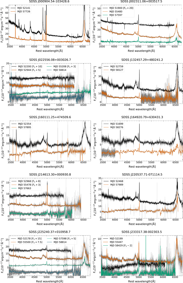
Figure 1. Original optical spectra of 10 changing-look quasars. See Table 1 for more details about the instruments and the transition directions. Noise is shown in gray. We apply a median filter to smooth the spectra for better visualization.
Download figure:
Standard image High-resolution imageTable 1. Optical Data of Changing-look Quasars
| Target Name | Redshift (z) | Instrument | Observation Date | Note | Transition |
|---|---|---|---|---|---|
| (1) | (2) | (3) | (4) | (5) | (6) |
| SDSS J000904.54-103428.6 | 0.2406 | SDSS | 52141 | Bright | Off |
| MMT | 57726 | Faint | |||
| SDSS J002311.06+003517.5 | 0.4221 | SDSS | 51900 | On/Off | |
| SDSS | 55480 | Bright | |||
| Magellan | 57597 | Faint | |||
| SDSS J022556.08+003026.7 | 0.5039 | SDSS | 52200 | On/Off/On | |
| SDSS | 52944 | Bright | |||
| SDSS | 55208 | Faint | |||
| ARC 3.5 m | 58814 | ||||
| SDSS J132457.29+480241.2 | 0.2716 | SDSS | 52759 | Bright | Off |
| HET | 58127 | Faint | |||
| SDSS J160111.25+474509.6 | 0.2970 | SDSS | 52354 | Bright | Off |
| MMT | 57895 | Faint | |||
| SDSS J164920.79+630431.3 | 0.3221 | SDSS | 51699 | Bright | Off |
| ARC 3.5 m | 58276 | Faint | |||
| SDSS J214613.30+000930.8 | 0.6220 | SDSS | 52968 | On/Off | |
| SDSS | 55478 | Bright | |||
| ARC 3.5 m | 57663 | Faint | |||
| SDSS J220537.71-071114.5 | 0.2950 | SDSS | 52468 | Bright | Off |
| MMT | 57989 | Faint | |||
| SDSS J225240.37+010958.7 | 0.5335 | SDSS | 52178 | On/Off | |
| SDSS | 55500 | Bright | |||
| Magellan | 57598 | ||||
| ARC 3.5 m | 58814 | Faint | |||
| SDSS J233317.38-002303.5 | 0.5130 | SDSS | 52199 | On/Off | |
| SDSS | 55447 | Bright | |||
| ARC 3.5m | 58429 | Faint |
Note. (1) Name of changing-look quasars in SDSS, in order of increasing R.A. (2) Spectroscopic redshift z, note that all 1σ uncertainties in spectroscopic redshifts are smaller than the last digit. (3) Instrument of observations. (4) Date of optical observations, in modified Julian date (MJD). (5) “Bright” denotes the brightest optical spectrum of the object, while “Faint” denotes the faintest optical spectrum of the object. (6) Transition direction(s) of changing-look quasars; “On” means that the changing-look quasar brightens (i.e., a “Turn-on” changing-look quasar), while “Off” means the changing-look quasar fades (i.e., a “Turn-off” changing-look quasar).
Download table as: ASCIITypeset image
To study the properties of the quasars while avoiding starlight contamination from their host galaxies, we use a Markov Chain Monte Carlo (MCMC) method to decompose every optical spectrum into a host galaxy spectrum and a quasar spectrum. We assume that these two spectra are linear combinations of galaxy/quasar eigenspectra. The galaxy and quasar eigenspectra are derived from principal component analysis based on 170,000 SDSS galaxy and 16,707 quasar spectra, respectively (Yip et al. 2004a, 2004b). We test selections of different numbers of galaxy and quasar eigenspectra used in the spectral decomposition, and find that seven galaxy eigenspectra and 18 quasar eigenspectra are sufficient to represent all the necessary features in our spectra. The second quasar eigenspectrum is not used in our decomposition, since it primarily represents a host galaxy component instead of a quasar spectrum (Yip et al. 2004b). We fit for the normalization factors of the first seven galaxy eigenspectra (Yip et al. 2004a), and 18 quasar eigenspectra (Yip et al. 2004b).
We perform Galactic extinction correction for all spectra before the decomposition (Cardelli et al. 1989; Schlegel et al. 1998). Due to the limited wavelength range of the eigenspectra, we only decompose spectra within the rest-frame wavelength range 3450–6800 Å.
To perform our fit, we use emcee v2.2.1 to run the MCMC (Foreman-Mackey et al. 2013), with a flat prior, and a logarithmic likelihood function:

where p is the likelihood, mi
is the fitted amplitude parameter for the i th eigenspectrum,  is the flux of ith eigenspectrum at the n th pixel in the spectrum, yn
is the flux of the observed spectrum at the nth pixel, and sn
2 is the variance of the observed spectrum at the nth pixel.
is the flux of ith eigenspectrum at the n th pixel in the spectrum, yn
is the flux of the observed spectrum at the nth pixel, and sn
2 is the variance of the observed spectrum at the nth pixel.
For the selected optical spectra of the same object (see Table 1), we decompose the two spectra together by assuming that their host galaxy spectra are the same shape. If more than two optical spectra are used in our analysis, for other optical spectra of that object, we subtract the best-fit host galaxy spectrum to derive their quasar spectrum. We present the decomposed spectra of SDSS J000904.54-103428.6 in Figure 2. We present decomposed spectra for our remaining targets in Appendix B.
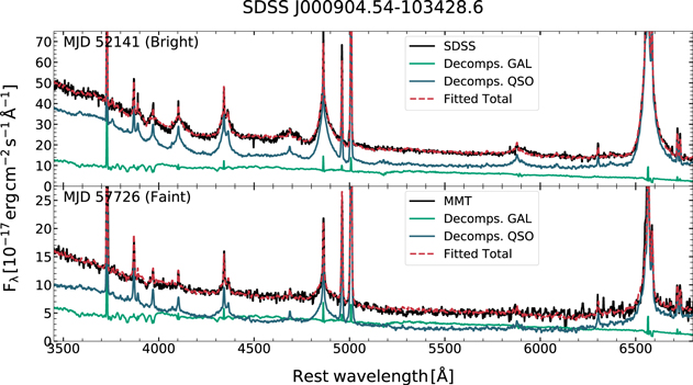
Figure 2. The decomposed spectra of SDSS J000904.54-103428.6. In each panel, we show the extinction-corrected observed spectrum in black. Noise is shown in gray. The decomposed host galaxy and the decomposed quasar spectrum are shown in green and blue, respectively. The red dashed line denotes the sum of the host galaxy and the quasar spectrum.
Download figure:
Standard image High-resolution imageFor every successful decomposition (i.e., the Markov Chain has converged), we subtract the derived host galaxy spectrum from the extinction-corrected, observed spectrum yielding the quasar spectrum used in the following analysis.
2.3. Quasar Spectrum Fitting
A quasar optical/UV spectrum can be represented by a power-law continuum and various emission lines (Vanden Berk et al. 2001). To investigate the properties of quasars, we need to measure the characteristic power-law index and the normalization of the continuum, as well as FWHMs of the broad emission lines. For the extracted quasar spectra, we use the MCMC (emcee v2.2.1 python package) method again (Foreman-Mackey et al. 2013), applying a flat prior, and a likelihood function:

where p is the likelihood,  is the flux of ith component at the nth pixel in the spectrum, yn
is the flux of the quasar spectrum at the nth pixel, and sn
2 is the variance of the observed spectrum at the nth pixel.
is the flux of ith component at the nth pixel in the spectrum, yn
is the flux of the quasar spectrum at the nth pixel, and sn
2 is the variance of the observed spectrum at the nth pixel.
We fit the quasar spectra with the following parameters:
- 1.Gaussian broad Balmer lines: heights, widths of
 -, and line centers of -. For most spectra in our analysis, their broad and can be fitted with one Gaussian function. However, there are some spectra showing more complex features in their broad and . The broad and lines of those quasars are fitted with two Gaussian functions, with heights, widths, and line centers as free parameters.
 - 2.Gaussian narrow emission lines: heights and widths of two Balmer lines and and forbidden lines [O iii] 4959, 5007, [N ii] 6548, 6584, and [S ii] 6717, 6731. We allow there to be a small wavelength offset () for all narrow emission lines due to uncertainties in spectroscopic redshifts or small wavelength shifts caused by imprecise wavelength calibration. We assume all the narrow lines have the same width ().
- 3.A Balmer continuum (Grandi 1982; Wills et al. 1985): The shape of the Balmer continuum depends sensitively on the optical depth but not on the electron temperature Te . Therefore, we assume Te = 15,000 K, and then calculate the Balmer continuum of optical depth from 0.1 to 2.0 with 0.1 spacing. The strength of the Balmer continuum is a parameter in our fit.
- 4.High-order Balmer lines: We adopt a high-order Balmer line model which includes energy levels from n = 8 to n = 50 in Storey & Hummer (1995) (Case B, electron temperature Te = 15,000 K, and electron density), and calculate a series of templates based on velocity from 1000 to 11,000 . We fit the normalization of the high-order Balmer line template.
- 5.Blended iron lines (Boroson & Green 1992): The contribution from Fe ii is also important for most quasars. We adopt the iron line template from Boroson & Green (1992) and fit its normalization. The width of the iron line template is associated with the FWHM of Hβ. During our analysis, we run a few test MCMCs to derive the FWHM of Hβ, and use the matched iron line template in the final MCMC (see below).
- 6.A power-law continuum: a power-law index and a normalization factor are fitted for the power-law continuum.
- 7.Some quasars have non-negligible broad helium emission lines, such as He ii λ4686 or/and He i λ5876. In this case, we also fit He ii λ4686 or/and He i λ5876 as broad Gaussian emission lines, and fit their strengths and widths with fixed line centers.





Since we do not correct telluric absorption for ARC 3.5 m spectra and MMT spectra, we mask some wavelength ranges in those spectra when performing the quasar spectral fitting, to avoid biases from telluric absorption. The masked wavelength ranges are shown as pink shaded regions in the figures of Appendix B.
We first run 20 separate test MCMCs for different optical depth Balmer continua from 0.1 to 2.0 by assuming the high-order Balmer line template and the iron line template associated with Hβ have an FWHM of 4500 km s−1. We find the lowest  among those 20 tests, and use the corresponding optical depth Balmer continuum in the final MCMC, and calculate the fitted
  FWHM. Then we find the high-order Balmer line and the iron line templates that most closely match that FWHM, and apply those high-order Balmer line and iron line templates in our final MCMC fit.
Since the high-order Balmer line model only includes energy levels to n = 50, there can be some discontinuity at ∼3600 Å between the Balmer continuum and high-order Balmer lines in our fitted spectra. A high-order Balmer line model with more energy levels can solve this issue (Kovačević et al. 2014; Kovačević-Dojčinović & Popović 2015). However, for the purposes of our work, a high-order Balmer line model with energy levels to n = 50 is adequate.
We obtain the best-fit power-law continuum luminosity at 2500 and 5100 Å (λ L2500 Å and λ L5100 Å), and their 1σ errors from the sample drawn from the MCMC. Based on the best-fit parameters and their 1σ errors, we use Monte Carlo resampling to generate 5000 profiles to calculate the uncertainties in the FWHM of broad Hβ, which is fitted with two Gaussian functions. For broad Hβ which can be fitted with a single Gaussian function, we directly use the best-fit width of broad Hβ to calculate its FWHM.
For each object, we choose a spectrum with a prominent broad Hβ emission line to measure its black hole mass, since broad Hβ is the best calibrated broad emission line from reverberation mapping (Peterson et al. 2004). We then measure the black hole mass based on the calculated FWHM of broad Hβ and λ L5100 Å, using the following equation (Greene et al. 2010):
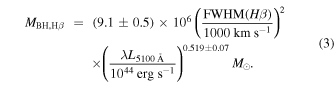
The errors of the black hole mass are calculated using propagation of errors in FWHM of Hβ and λ L5100 Å.
We present our best-fit power-law indices, best-fit power-law normalizations, λ
L2500 Å, λ
L5100
Å, FWHM of  , and black hole mass
  in Table 2. We also provide the fiducial black hole mass measurement from Shen et al. (2011) for comparison; the latter incorporates black hole mass prescriptions and measurements from previous works (McLure & Dunlop 2004; Vestergaard & Peterson 2006; Vestergaard & Osmer 2009; Shen et al. 2011). Our measured results are consistent with their measurements within 1σ errors or within 0.4 dex, the intrinsic scatter in mass scaling relationship of broad emission lines (Vestergaard & Peterson 2006), except for SDSS J233317.38-002303.5. For this object, we adopt a different SDSS spectrum than Shen et al. (2011) to measure its black hole mass, in which the broad Hβ emission is more prominent, and thus we adopt our measured black hole mass as the black hole mass of SDSS J233317.38-002303.5 in the following analysis.
Table 2. Best-fit Results of Optical Changing-look Quasar Spectra
| Target Name | Obs. Date | PL Index | PL Norm. |

|

| FWHM (H ) ) |

| Ref. 
|
|---|---|---|---|---|---|---|---|---|
| (SDSS) | (MJD) |

|

|

| ( ) ) | ( ) ) | ( ) ) | |
| (1) | (2) | (3) | (4) | (5) | (6) | (7) | (8) | (9) |
| J000904.54-103428.6 | 52141 |

|

|

|

|

|

|

|
| 57726 |

|

|

|

| ||||
| J002311.06+003517.5 | 51900 |

|

|

|

|

|

|

|
| 55480 |

|

|

|

| ||||
| 57597 |

|

|

|

| ||||
| J022556.08+003026.7 | 52200 |

|

|

|

| |||
| 52944 |

|

|

|

|

|

|

| |
| 55208 |

|

|

|

| ||||
| 58814 |

|

|

|

| ||||
| J132457.29+480241.2 | 52759 |

|

|

|

|

|

|

|
| 58127 |

|

|

|

| ||||
| J160111.25+474509.6 | 52354 |

|

|

|

|

|

|

|
| 57895 |

|

|

|

| ||||
| J164920.79+630431.3 | 51699 |

|

|

|

|

|

|

|
| 58276 |

|

|

|

| ||||
| J214613.30+000930.8 | 52968 |

|

|

|

|

| ||
| 55478 |

|

|

|

|

|

| ||
| 57663 |

|

|

|

| ||||
| J220537.71-071114.5 | 52468 |

|

|

|

|

|

|

|
| 57989 |

|

|

|

| ||||
| J225240.37+010958.7 | 52178 |

|

|

|

|

| ||
| 55500 |

|

|

|

|

|

| ||
| 57598 |

|

|

|

| ||||
| 58814 |

|

|

|

| ||||
| J233317.38-002303.5 | 52199 |

|

|

|

| |||
| 52525 | - | - | - | - | - | - |

| |
| 55447 |

|

|

|

|

|

| ||
| 58429 |

|

|

|

|
Note.(1) Name of CLQs in SDSS. (2) Date of optical observations in MJD. (3)–(4) The best-fit power-law index and normalization of the power-law continuum. (5) The monochromatic luminosity of the power-law continuum at 2500 Å. (6) The monochromatic luminosity of the power-law continuum at 5100 Å. (7) The FWHM of broad Hβ. (8) The measured black hole mass. (9) The referenced black hole mass is adopted from the fiducial black hole mass in Shen et al. (2011). All the errors represent 1σ confidence intervals.
Download table as: ASCIITypeset image
In Figure 3, we show our spectral fitting of SDSS J000904.54-103428.6. Spectral fittings of other objects are included in Appendix B.
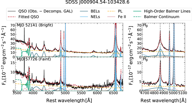
Figure 3. The spectral fitting of SDSS J000904.54-103428.6. The quasar spectrum is in black. The best-fit broad and narrow emission lines are shown in dark and light blue, respectively. The best-fit power-law continuum and blended iron lines are denoted by a yellow dashed line and a pink line. High-order Balmer lines and the Balmer continuum are in solid green and dashed green lines. The red dashed line represents the sum of the fitted models. Left: spectral fitting in 3,450−6,800 Å. Right: spectral fitting around  . Wavelength of fitted narrow
  , [O iii]
  4959,5007 emission lines are denoted by vertical dashed lines.
Download figure:
Standard image High-resolution image3. X-Ray Data
For our X-ray analysis of CLQs, we search the XMM-Newton data archive, and obtain new Chandra Cycle 19 observations. The new Chandra and archival XMM-Newton observations are close in time to our new optical spectra, and thus it is likely that they reflect the X-ray properties of the same states as the optical spectra. Further discussion about the uncertainties on  caused by the time difference between optical and X-ray observations can be found in Section 4.2.
We also used X-ray data from the ROSAT data archive to constrain the X-ray flux of changing-look quasars close in time to their first optical observations from SDSS. The ROSAT observations were obtained approximately 10 yr before the first SDSS observations; we use them only to loosely constrain the X-ray flux associated with the first SDSS observation of each CLQ. Of course, these CLQs could have changed their X-ray fluxes within these 10 yr. Therefore, we only tentatively connect ROSAT X-ray fluxes with the early optical data, and present our results in Appendix A.
3.1. Chandra Observations
We obtained new Chandra Cycle 19 ACIS-S observations (ObsID 20459−20468) to measure the X-ray properties of quasars associated with the new optical spectra (PI: Ruan; Program NO: 19700565). Each observation has an exposure time of at least 4 ks, up to ∼20 ks, and is in “VFAINT” mode to ensure the best sensitivity, with the targeted quasar located at the aim point of ACIS-S3 chip. We use Chandra Interactive Analysis of Observations (CIAO) v4.10 (CALDB v4.7.9) for data reduction (Fruscione et al. 2006). We reprocess level-1 data with the calibration files, following the standard data reduction procedure. We check each light curve, and find there was no significant particle flare during the observation. We produce a 0.3–8 keV counts map of each observation and use wavdetect to perform source detection. The targeted quasar is detected in every data set. Due to possible physical offsets between the optical and X-ray center or limited pointing accuracy, there can be some small offsets (≲2″) between the coordinates detected by SDSS and Chandra. For this reason, we use X-ray source coordinates detected by wavdetect as the source centers when extracting spectra with specextract. The source counts are extracted within 5″ of each source’s center, and the corresponding background counts are extracted from a 40″ to 50″ annulus. To avoid point-source contamination in the background region, we use a 20″–30″ annulus for SDSS J132457.29+480241.2 and SDSS J160111.25+474509.6 for the extraction of background counts.
For four sources that have sufficient 0.5–7.0 keV counts (≳150; Evans et al. 2010), we group the X-ray counts into 15 per bin and use Xspec v12.10.1 to perform spectral fits (Arnaud 1996), assuming an absorbed power law with a fixed Galactic absorption (wabs*powerlaw; Morrison & McCammon 1983). We present the best-fit results in Table 3, and we present the X-ray spectra in Figure 4, with the models superposed. We then calculate the 0.5–7.0 keV energy flux, based on the best-fit results. For the other six CLQs, their X-ray counts are not sufficient to perform X-ray spectral fitting. We instead measure their 0.5–7.0 keV count rate, and then convert the 0.5–7.0 keV count rate into the 0.5–7.0 keV energy flux by assuming a photon index of 1.8, which is the median X-ray power-law photon index from BAT AGN Spectroscopic Survey (BASS; Trakhtenbrot et al. 2017), and a fixed Galactic absorption. We calculate their rest-frame 2 keV flux density using the Chandra WebPIMMs
16
tool. We list our measured rest-frame 2 keV luminosity ( ) in Table 3.
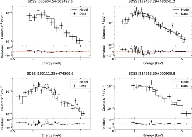
Figure 4. Chandra spectra of four changing-look quasars. Every upper panel shows the best-fit model and the observed X-ray spectrum, and each lower panel displays the residuals.
Download figure:
Standard image High-resolution imageTable 3. X-Ray Properties of Changing-look Quasars
| Target Name | Instrument | Observation Date | Exp. | Count Rate | Photon Index |

|
|---|---|---|---|---|---|---|
| (SDSS) | (MJD) | (ks) |

|

| ||
| (1) | (2) | (3) | (4) | (5) | (6) | (7) |
| J000904.54-103428.6 | Chandra | 58363 | 11.9 | 1.7 ± 0.1 | 1.7±0.2 a |

|
| J002311.06+003517.5 | Chandra | 58254 | 4.0 | 3.7 ± 0.3 | 1.8 | 140 ± 12 |
| J022556.08+003026.7 | Chandra | 58182 | 7.0 | 0.6 ± 0.1 | 1.8 | 39 ± 6 |
| J132457.29+480241.2 | Chandra | 58385 | 13.9 | 4.8 ± 0.2 |
 a
a
|

|
| J160111.25+474509.6 | Chandra | 58359 | 17.8 | 3.0 ± 0.1 | 1.8±0.1 a | 44 ± 2 |
| J164920.79+630431.3 | Chandra | 58213 | 22.8 | 0.47 ± 0.05 | 1.8 | 8.8 ± 0.9 |
| J214613.30+000930.8 | Chandra | 58230 | 11.9 | 2.0 ± 0.1 |
 a
a
|

|
| J220537.71-071114.5 | Chandra | 58023 | 18.8 | 0.65 ± 0.06 | 1.8 | 9.5 ± 0.9 |
| J225240.37+010958.7 | XMM-Newton | 57559 | 9.3 | 1.5 ± 0.2 |
 a
a
|

|
| Chandra | 58027 | 8.0 | 1.1 ± 0.1 | 1.8 | 77 ± 8 | |
| J233317.38-002303.5 | XMM-Newton | 56072 | 3.7 | 11.4 ± 0.6 | 2.1±0.1 a |

|
| Chandra | 58256 | 7.0 | 1.3 ± 0.1 | 1.8 | 87 ± 9 |
Note. (1) Name of CLQs in SDSS. (2) Instrument of X-ray observations. (3) Date of X-ray observations in MJD. (4) Exposure time in kiloseconds (ks). XMM-Newton observations only include the PN instrument exposure time. (5) 0.5–7 keV count rate in units of  . (6) Best-fit photon index. 1.8 is for the sources that do not have enough counts to perform X-ray spectral fitting. (7) Unabsorbed rest-frame 2 keV luminosity, in units of
  , calculated by Chandra WebPIMMs by assuming a fixed galactic absorption and a photon index in column (6). All the errors are 1σ.
Download table as: ASCIITypeset image
3.2. Archival XMM-Newton Data
We search for additional archival X-ray observations and find that SDSS J225240.37+010958.7 and SDSS J233317.38-002303.5 were previously observed with XMM-Newton. Due to the existence of nearly contemporaneous optical observations with the XMM-Newton observations, we include these two XMM-Newton observations in our analysis. To ensure the best spectral resolution, we only use the data from the PN instrument. We use the Science Analysis System (SAS) v17.0.0 to reduce the XMM-Newton PN observations with newly calibrated files, following the SAS Threads, and reprocess the observation data files with epproc. We then use evselect to filter the event lists for flaring particle background. We adopt a circular source region of 32″ radius, and use the same CCD chip to measure the background from a region of the same size without any discrete sources. We then use evselect to extract the corresponding spectrum. A redistribution matrix and an ancillary file are generated based on the extracted spectra by rmfgen and arfgen. We group the X-ray counts into 15 counts per bin and use Xspec v12.10.1 to perform X-ray spectral fitting. We fit an absorbed power law (wabs*powerlaw) to the extracted spectra, accounting for a fixed Galactic absorption. We present our fitted results in Table 3 and the fitted spectrum in Figure 5. The 0.5–7 keV energy flux is calculated based on the best-fit results, and then we calculate the rest-frame 2 keV flux density using the Chandra WebPIMMs tool, and present rest-frame 2 keV luminosity ( ) in Table 3.
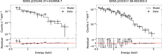
Figure 5. The XMM-Newton spectra of SDSS J225240.37+010958.7 and SDSS J233317.38-002303.5. The observed X-ray spectrum and the best-fit model are in every upper panel, and every lower panel displays the residuals.
Download figure:
Standard image High-resolution image4. Results and Discussion
4.1.

We use the Chandra and XMM-Newton X-ray data together with optical measurements that are close in time to analyze the optical/X-ray spectral shapes.
We also leverage the earliest optical measurements with X-ray flux constraints derived from the ROSAT PSPC all-sky survey. We emphasize that due to the large difference between the time of the earliest SDSS observations and ROSAT observations, these measurements should be regarded as crude constraints on  . We present these results using ROSAT observations in Appendix A.
We use the following definition to calculate the optical/X-ray spectral index  (Tananbaum et al. 1979):

where the monochromatic 2500 Å luminosity ( ) is calculated by extrapolating the best-fit power-law continuum to 2500 Å in the rest-frame (see Table 2), and the rest-frame 2 keV luminosity (
 ) is calculated as in Section 3 (see Table 3).
We then use the 2–10 keV luminosity and  to obtain the bolometric luminosity, with the following bolometric correction (Lusso et al. 2010):

where L[2–10]
keV is the rest-frame 2–10 keV luminosity. L[2–10]
keV is calculated based on the best-fit X-ray spectrum if there are enough X-ray counts in that observation, otherwise it is calculated by assuming an X-ray photon index of 1.8. We then calculate the Eddington ratio ( ) as the ratio of the bolometric luminosity to the Eddington luminosity, i.e.,
  , where
  . We present the measured
  values and Eddington ratios in Table 4.
Table 4. Measured  and
and  of Changing-look Quasars
| Target Name (SDSS) | Optical MJD | X-Ray MJD |

|

| Label |
|---|---|---|---|---|---|
| (1) | (2) | (3) | (4) | (5) | (6) |
| J000904.54-103428.6 | 57726 | 58363 |

|

| A |
| J002311.06+003517.5 | 57597 | 58254 |

|

| B |
| J022556.08+003026.7 | 58814 | 58182 |

|

| C |
| J132457.29+480241.2 | 58127 | 58385 |

|

| D |
| J160111.25+474509.6 | 57895 | 58359 |

|

| E |
| J164920.79+630431.3 | 58276 | 58213 |

|

| F |
| J214613.30+000930.8 | 57663 | 58230 |

|

| G |
| J220537.71-071114.5 | 57989 | 58023 |

|

| H |
| J225240.37+010958.7 | 57598 | 57559 |

|

| I1 |
| 58814 | 58027 |

|

| I2 | |
| J233317.38-002303.5 | 55447 | 56072 |

|

| J1 |
| 58429 | 58256 |

|

| J2 |
Note. (1) Name of CLQs in SDSS. (2) MJD of the optical data, see Table 1 for details. (3) MJD of the X-ray data, see Table 3 for details. (4) Optical/UV–X-ray spectral indices  (
( can be found in Table 2, and
  can be found in Table 3). (5) Logarithmic Eddington ratio
  , using a bolometric luminosity calculated with optical data and X-ray data (i.e., Equation (5)). (6) Label of green square data points presented in Figure 6. All error bars denote 1σerrors.
Download table as: ASCIITypeset image
Figure 6 presents our measurements of  and
and  . We include measurements of six “turn-off” CLQs from Ruan et al. (2019a) as well. We compare these measurements with results of simulations from Sobolewska et al. (2011). Sobolewska et al. (2011) use a multicolor blackbody model (DISKBB; Mitsuda et al. 1984) for the emission from the accretion disk and a Comptonization model (EQPAIR; Coppi 1999) for the coronal emission to fit the X-ray spectrum of the black hole X-ray binary GRO J1655-40 during its outburst in 2005. This analysis assumes the emission from the accretion disk and the corona can be directly scaled by black hole masses at the same Eddington ratio (for a Shakura–Sunyaev disk, the scaling relation between the accretion disk temperature and the black hole mass is
  ), and it scales the emission from this stellar mass black hole to the supermassive black hole case with a mass distribution from the zCOSMOS survey (Merloni et al. 2010). It predicts a positive correlation between
  and
and  at Eddington ratios ≳1%, a critical Eddington ratio 1%, following the critical Eddington ratio of X-ray binaries (Maccarone 2003), and an anticorrelation between
  and
and  at low Eddington ratios ≲1%.
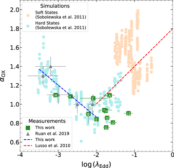
Figure 6. Measured  and
and  of changing-look quasars. Green squares are measurements of 10 changing-look quasars in this work (see Table 4 for more details). Labels of individual changing-look quasars can be found in column (6) of Table 4. Latest measurements of
  and
and  from Ruan et al. (2019a) are denoted by gray triangles. The blue dashed line displays the fitted
  relation (i.e., Equation (6)) at
  from this work and Ruan et al. (2019a). The
  relation of bright quasars derived from the XMM-COSMOS survey is shown by the red dashed line (Lusso et al. 2010). Peach and turquoise hexagons are simulated results from Sobolewska et al. (2011), based on RXTE observations of the black hole X-ray binary GRO J1655-40.
Download figure:
Standard image High-resolution imageOur measurements are generally consistent with the simulations of Sobolewska et al. (2011). At  , there is also an observed positive correlation between
  and
and  (Maoz 2007; Lusso et al. 2010; Grupe et al. 2010). This relation given by the XMM-COSMOS survey (Lusso et al. 2010) is
  . The null hypothesis is rejected at the ∼9σ confidential level. At
  ,
,  and
and  show an anticorrelation, and the Pearson correlation coefficient is −0.85. For 11 measurements at
  (in this work and Ruan et al. 2019a), we use linear regression analysis, considering measurement errors in both
  and
and  (i.e., the bivariate correlated errors and intrinsic scatter [BCES] method; see Akritas & Bershady 1996; Nemmen et al. 2012), to fit the relation between
  and
and  . Our fitted result (bisector) is:

This anticorrelation
17
again suggests similarities in the spectral indices below 1%  between CLQs and X-ray binaries undergoing accretion state transitions. Though the transition timescale of CLQs is not consistent with the expected accretion state transition timescale for AGN (∼105 yr), Noda & Done (2018) suggest that in AGN, radiation pressure and magnetic pressure can play more important roles than in X-ray binaries, which can dramatically reduce the variability timescale.
4.2. Sources of Uncertainty in

In Table 4, the uncertainties in  are from propagation of uncertainties in measured
  (reported in Table 2) and
  (reported in Table 3). However, there are additional sources of uncertainties in
  . We briefly discuss them here:
- 1.Selection of photon indices: For sources that do not have sufficient X-ray counts for spectral fitting, we assume a photon index 1.8 to calculate the rest-frame 2 keV luminosity. The assumption of different photon indices will result in different , and thus we investigate the possible uncertainty in . We adopt the photon index distribution from BASS, which has a mean value 1.8, and a standard deviation 0.27 (Trakhtenbrot et al. 2017). We thus use different photon indices (1.53, 1.8, and 2.07) to calculate , and we find they are consistent with 6%, which will change by only 0.01.
- 2.Time difference between optical and X-ray observations: The observation dates of X-ray (Chandra or XMM-Newton) and optical data are close but not exactly the same, which can also cause uncertainty in. The maximal time lag between optical and X-ray observation dates in the rest-frame is ∼500 days (∼1.4 yr). Since there are no existing studies of CLQ optical and X-ray variability over a yearly timescale, to investigate the uncertainty in , we instead use the structure function (SF) for quasar variability in 2000–3000 Å (MacLeod et al. 2012), and we find the corresponding average SF in mag is 0.2 for a rest-frame time lag of 500 days. For the uncertainty in , we use an X-ray structure function for quasar variability in 0.2–2 keV band (Middei et al. 2017), and we find the average SF for a rest-frame time lag of 1.4 yr is ∼0.23 in a base-10 log scale. Combining these two uncertainties and using the propagation of errors, we estimate that a rest-frame time lag of 500 days between the optical and X-ray observations can change up to 0.09.


Based on the estimation of these two uncertainties, we fit the  relation by including an extra uncertainty of 0.09 in
  , apart from the given uncertainties in
  in Table 4. The fitted result from BCES (bisector) is
  The slope is consistent with the slope in Equation (6) within 1σ errors. However, the fitted linear relation of only five data points below
  in this work becomes
  . Therefore, more measurements below
  are still required to derive a more robust
  relation in this regime.
4.3. Changes in the BLR Associated with Changes in

To study the changes in Eddington ratios of CLQs, associated with changes in their broad emission lines, we select the brightest and faintest optical spectra, and measure their Eddington ratios.
For every object, we define the brightest optical spectrum as the “bright” state, while the faintest optical spectrum as the “faint” state, as shown in Table 1. For nine bright states and for one faint state, contemporaneous X-ray observations are not directly available. To avoid systematic offsets, we calculate all the bolometric luminosity with only optical data, by adopting a linear bolometric correction (Runnoe et al. 2012):

The Eddington ratio is then calculated as the ratio of the bolometric luminosity to the Eddington luminosity.
We present all the measured Eddington ratios in Table 5. To study distributions of Eddington ratios in the bright and faint states, we use extreme deconvolution to derive the underlying distributions that are convolved with the statistical uncertainties to produce the observed Eddington ratio values (Bovy et al. 2011). To obtain a larger data sample of CLQs, we include the measurements of six “turn-off” CLQs in Ruan et al. (2019a) to derive a more robust result. They adopt a different bolometric correction than our work, so we recalculate Eddington ratios of these six CLQs in both bright and faint states, based on their reported  . We assume the distribution in Eddington ratios of the bright and faint states can be described by Gaussian mixtures in a logarithmic scale of Eddington ratios. We then use the XDGMM (Holoien et al. 2017) package to calculate the Bayesian information criterion (BIC; Schwarz 1978) for the Gaussian mixtures with different numbers of Gaussian functions from 1 to 10. We find that fitting with a single Gaussian function has the lowest BIC for both bright and faint states, and thus we use a single Gaussian function to fit the Eddington ratio distributions of both states and resample these two distributions with corresponding errors.
Table 5. Measured  of Bright and Faint State Changing-look Quasars
| Target Name (SDSS) | State | Optical MJD |

|
|---|---|---|---|
| (1) | (2) | (3) | (4) |
| J000904.54-103428.6 | Bright | 52141 |

|
| Faint | 57726 |

| |
| J002311.06+003517.5 | Bright | 55480 |

|
| Faint | 57597 |

| |
| J022556.08+003026.7 | Bright | 52944 |

|
| Faint | 55208 |

| |
| J132457.29+480241.2 | Bright | 52759 |

|
| Faint | 58127 |

| |
| J160111.25+474509.6 | Bright | 52354 |

|
| Faint | 57895 |

| |
| J164920.79+630431.3 | Bright | 51699 |

|
| Faint | 58276 |

| |
| J214613.30+000930.8 | Bright | 55478 |

|
| Faint | 57663 |

| |
| J220537.71-071114.5 | Bright | 52468 |

|
| Faint | 57989 |

| |
| J225240.37+010958.7 | Bright | 55500 |

|
| Faint | 58814 |

| |
| J233317.38-002303.5 | Bright | 55447 |

|
| Faint | 58429 |

|
Note. (1) Name of CLQs in SDSS. (2) “Bright” denotes the brightest optical spectrum among all the optical spectra of the same object, while “Faint” denotes the faintest optical spectrum. (3) MJD of the optical data, see Table 1 for details. (4) Logarithmic Eddington ratio, using a bolometric luminosity calculated with only optical data (i.e., Equation (7),  and
and  can be found in Table 2). All error bars denote 1σ errors.
Download table as: ASCIITypeset image
Figure 7 displays the distributions of bright and faint state Eddington ratios. The original Eddington ratio distributions are in solid histograms. We also directly calculate the mean values and the standard deviations of bright and faint state Eddington ratios without uncertainties, and show them as dotted single Gaussian functions. The best-fit mean values of the two distributions from the XDGMM lay above and below the 1% Eddington ratio value, which is close to the critical Eddington ratios observed for many X-ray binaries undergoing accretion state transitions. Furthermore, from the bright state to the faint state, broad emission lines in the optical spectra significantly dim, and thus the best-fit mean Eddington ratios of the bright state to the faint state cross 1% Eddington ratio. The disk-wind model predicts dramatic fading of the broad emission lines below the 1% Eddington ratio (Elitzur & Netzer 2016). This is in good agreement with the measured Eddington ratios of CLQs from their bright state to their faint state, when their broad emission lines have dimmed significantly.
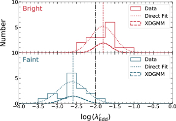
Figure 7. The distributions of Eddington ratios of bright and faint state changing-look quasars in this work and in Ruan et al. (2019a) are shown in the upper and lower panels, respectively. The original bright and faint state distributions are shown in the solid histograms. The means and widths of the dotted Gaussian functions are derived from average Eddington ratios and standard deviations of Eddington ratios, without any uncertainties. The normalized resampled distributions from the extreme deconvolution method (XDGMM) are shown in the thick dashed lines. Best-fit mean values from XDGMM are denoted by vertical thin dashed lines of corresponding color. The black dashed–dotted line denotes the critical Eddington ratio of 1%, predicted by the disk-wind model.
Download figure:
Standard image High-resolution imageWe further test whether this result will change when calculating Eddington ratios with a different bolometric correction. The linear bolometric correction (Equation (7)) is derived from bright quasars (Runnoe et al. 2012), and assumes the same SED shape for quasars at different Eddington ratios. This assumption should not be problematic for CLQs in the bright state, but might be biased for CLQs in the faint state, considering the SED shape changes at different Eddington ratios (Ho 1999; Vasudevan & Fabian 2007; Ho 2009; Vasudevan & Fabian 2009). We thus investigate nine faint state CLQs with sensitive X-ray data from Chandra, and calculate their Eddington ratios with both optical and X-ray data (Equation (5), see the column (5) in Table 4). We find this bolometric correction results in higher Eddington ratios for the nine faint states by 0.5 dex on average. Applying this shift to the best-fit mean value of the faint state, we find the mean value of the faint state is still below the 1% Eddington ratio. Thus, even when using a different bolometric correction, the mean of the Eddington ratio distributions in the bright and faint states still crosses the 1% value in Eddington ratio.
Apart from the critical 1% Eddington ratio, the disk-wind model also suggests that emission line profiles characteristic of a disk origin (flat-topped, red-asymmetric, and/or double-peaked) are expected for intermediate type AGN (Chiang & Murray 1996; Murray & Chiang 1997; Flohic et al. 2012; Chajet & Hall 2013; Elitzur et al. 2014). Two of our 10 CLQs (SDSS J022556.08+003026.7 and J225240.37+010958.7) in this study show a weak double-peaked feature in their broad Hβ emission line (see Appendix B), which may support the disk-wind model as the origin of broad emission lines. For the other eight CLQs, we do not detect a double-peaked broad emission line. This might be attributed to the low signal-to-noise ratio spectra or lack of spectroscopy when those CLQs faded. Multiepoch, high-quality spectra of CLQs are still needed to study the transformation in their emission line profiles in detail, and to further investigate the connection with the disk-wind model.
5. Conclusion
In this paper, we present optical and X-ray measurements of 10 CLQs. By comparing their  and
and  with simulated results from Sobolewska et al. (2011), based on RXTE observations of a black hole X-ray binary, we find similar trends in spectral index changes between X-ray binaries in accretion state transitions in low/hard states and CLQs below 1% Eddington ratios. This result bolsters the idea that quasars have analogous flows with those in X-ray binaries. This
  and
and  anticorrelation below 1%
  is also found by multiepoch Swift observations of the changing-look AGN NGC 2617 (Ruan et al. 2019b). Furthermore, by measuring the Eddington ratios of CLQs before/after they show changes in broad emission lines, we find that CLQs appear to cross the 1% Eddington ratio value when the strength of their broad emission lines changes drastically. Future multiepoch observations and spectroscopy on individual CLQs may be able to investigate the disk-wind model in more detail, and shed more light on the origin of broad emission lines.
We thank the anonymous reviewer for helpful and informative comments that improved and clarified this manuscript. X.J., J.J.R., and D.H. acknowledge support from an NSERC Discovery Grant, a FRQNT Nouveaux Chercheurs Grant, and support from the Canadian Institute for Advanced Research (CIFAR). J.J.R, S.F.A., A.D., and M.E. are supported by Chandra Award Number GO7-18033X and GO8-19090A, issued by the Chandra X-ray Observatory center, which is operated by the Smithsonian Astrophysical Observatory for and on behalf of the National Aeronautics Space Administration (NASA) under contract NAS8-03060. C.L.M, P.J.G., S.F.A., and J.J.R. are supported by the National Science Foundation under Grants No. AST-1715763 and AST-1715121. J.J.R. acknowledges funding from the McGill Trottier Chair in Astrophysics and Cosmology, the McGill Space Institute, and the Dan David Foundation.
The scientific results reported in this article are based to a significant degree on observations made by the Chandra X-ray Observatory, and the Chandra Data Archive.
This work uses the ROSAT Data Archive of the Max-Planck-Institut für extraterrestrische Physik (MPE) at Garching, Germany. This work also uses observations obtained with XMM-Newton, an ESA science mission with instruments and contributions directly funded by ESA member states and NASA.
This work uses observations obtained with the Apache Point Observatory 3.5 m telescope, which is owned and operated by the Astrophysical Research Consortium.
This work uses observations obtained at the MMT Observatory, a joint facility of the Smithsonian Institution and the University of Arizona.
This paper includes data gathered with the 6.5 meter Magellan Telescopes located at Las Campanas Observatory, Chile.
This work uses observations obtained with the Hobby–Eberly Telescope and The Low Resolution Spectrograph 2. The Hobby–Eberly Telescope (HET) is a joint project of the University of Texas at Austin, the Pennsylvania State University, Stanford University, Ludwig-Maximillians-Universität Munchen, and Georg-August-Universität Göttingen. The HET is named in honor of its principal benefactors, William P. Hobby and Robert E. Eberly.
The Low Resolution Spectrograph 2 (LRS2) was developed and funded by the University of Texas at Austin McDonald Observatory and Department of Astronomy and by The Pennsylvania State University. We thank the Leibniz-Institut für Astrophysik Potsdam (AIP) and the Institut für Astrophysik Göttingen (IAG) for their contributions to the construction of the integral field units.
Funding for the Sloan Digital Sky Survey IV has been provided by the Alfred P. Sloan Foundation, the U.S. Department of Energy Office of Science, and the Participating Institutions. The SDSS-IV acknowledges support and resources from the center for High-Performance Computing at the University of Utah. The SDSS website is www.sdss.org.
The SDSS-IV is managed by the Astrophysical Research Consortium for the Participating Institutions of the SDSS Collaboration, including the Brazilian Participation Group, the Carnegie Institution for Science, Carnegie Mellon University, the Chilean Participation Group, the French Participation Group, the Harvard-Smithsonian Center for Astrophysics, Instituto de Astrofísica de Canarias, The Johns Hopkins University, the Kavli Institute for the Physics and Mathematics of the Universe (IPMU)/University of Tokyo, the Korean Participation Group, Lawrence Berkeley National Laboratory, Leibniz Institut für Astrophysik Potsdam (AIP), Max-Planck-Institut für Astronomie (MPIA Heidelberg), Max-Planck-Institut für Astrophysik (MPA Garching), Max-Planck-Institut für Extraterrestrische Physik (MPE), National Astronomical Observatories of China, New Mexico State University, New York University, the University of Notre Dame, Observatório Nacional/MCTI, The Ohio State University, Pennsylvania State University, the Shanghai Astronomical Observatory, the United Kingdom Participation Group, Universidad Nacional Autónoma de México, the University of Arizona, the University of Colorado Boulder, the University of Oxford, the University of Portsmouth, the University of Utah, the University of Virginia, the University of Washington, the University of Wisconsin, Vanderbilt University, and Yale University.
IRAF is distributed by the National Optical Astronomy Observatory, which is operated by the Association of Universities for Research in Astronomy (AURA) under a cooperative agreement with the National Science Foundation.
Facilities: SDSS - , MMT - , Magellan Telescope - , ARC 3.5m - , HET - , ROSAT - , XMM (PN) - , CXO (ACIS-S). -
Software: CIAO (Fruscione et al. 2006), SAS (https://www.cosmos.esa.int/web/xmm-newton/what-is-sas), XIMAGE (https://heasarc.gsfc.nasa.gov/docs/xanadu/ximage), XSPEC (Arnaud 1996), Chandra WebPIMMs (https://cxc.harvard.edu/toolkit/pimms.jsp), IRAF (Tody 1986, 1993), emcee (Foreman-Mackey et al. 2013), XDGMM (Holoien et al. 2017), Astropy (Astropy Collaboration et al. 2013, 2018), Matplotlib (Hunter 2007), BCES (Akritas & Bershady 1996; Nemmen et al. 2012).
Appendix A: Early X-Ray Constraints from ROSAT
We obtain constraints in X-ray fluxes from ROSAT, and connect them with the earliest SDSS observations to measure  . Note that the time lag between optical and ROSAT X-ray observations is around 10 yr, which is comparable to the timescale on which CLQs have been observed to change spectral types. Therefore, those
  measurements should be viewed as crude constraints. In the following part of this section, we summarize the ROSAT observations and present
  from the ROSAT observations and the earliest optical observations.
We first search the coordinates of CLQs with a default 1′ matching radius in the second ROSAT all-sky survey source catalog (2RXS; Boller et al. 2016), which is the newest public source catalog derived from ROSAT position-sensitive proportional counter (PSPC) all-sky survey. The typical observation date of ROSAT PSPC observations is around 1990/1991, which is ∼10 yr before the first SDSS spectra of our CLQs. Three sources (SDSS J000904.54-103428.6, SDSS J002311.06+003517.5 and SDSS J132457.29+480241.2) were detected by the 2RXS catalog. We adopt their 0.1–2.4 keV count rate reported in the 2RXS catalog in our analysis.
For the remaining sources, we acquire 0.1–2.4 keV photon images and exposure maps from the ROSAT PSPC all-sky survey, and use the SOSTA tool in XIMAGE
18
to extract the 0.1–2.4 keV count rate. We convert the 0.1–2.4 keV count rate into the rest-frame 2 keV flux density using the Chandra WebPIMMs tool with an assumed photon index of 1.8. For the sources that were not detected by ROSAT (i.e., signal-to-noise ratio  ), we instead calculate their 3σupper limit on the 0.1–2.4 keV count rate, and set a 3σupper limit on the rest-frame 2 keV luminosity
  . We present our measurements in Table 6.
Table 6. X-Ray Properties of Changing-look Quasars from ROSAT
| Target Name | Observation Date | Exp. | Count Rate | Ref. |

|
|---|---|---|---|---|---|
| (SDSS) | (MJD) | (ks) | (10−2 cts s−1) | (1042 erg s−1) | |
| (1) | (2) | (3) | (4) | (5) | (6) |
| J000904.54-103428.6 | 48225 | 0.4 | 9 ± 2 | 2RXS | 140 ± 30 |
| J002311.06+003517.5 | 48083 | 0.4 | 4 ± 1 | 2RXS | 260 ± 70 |
| J022556.08+003026.7 | 48266 | 0.2 | <10 | <1000 | |
| J132457.29+480241.2 | 48214 | 0.6 | 14 ± 2 | 2RXS | 200 ± 30 |
| J160111.25+474509.6 | 48083 | 0.5 | 41 ± 14 | 800 ± 300 | |
| J164920.79+630431.3 | 48083 | 2.7 | <13 | <400 | |
| J214613.30+000930.8 | 48193 | 0.3 | <28 | <6600 | |
| J220537.71-071114.5 | 48197 | 0.1 | <64 | <1900 | |
| J225240.37+010958.7 | 48292 | 0.3 | <32 | <4900 | |
| J233317.38-002303.5 | 48224 | 0.3 | <18 | <2300 |
Note. (1) Name of CLQs in SDSS. (2) Date of X-ray observations in MJD. (3) Exposure time in kiloseconds (ks). ROSAT observations are from the PSPC all-sky survey; therefore, they have relatively shallow exposure. (4) 0.1–2.4 keV count rate in units of 10−2 cts s−1. (5) Reference for count rates in (4). 2RXS represents the “Second ROSAT all-sky Survey Source Catalogue” (Boller et al. 2016). If it is not specified, the count rate is measured from our work. (6) Unabsorbed rest-frame 2 keV luminosity, in units of 1042 erg s−1, calculated by Chandra WebPIMMs by assuming a fixed galactic absorption and a photon index of 1.8. All the errors are 1σ, and all the upper limits are 3σ.
Download table as: ASCIITypeset image
We connect the ROSAT observations with the earliest optical observations from SDSS. We then calculate  based on Equation (4). For those measurements, the ROSAT observations predate the optical spectra by ≳10 yr. Thus, we can only measure the bolometric luminosity from the optical data, by adopting a linear bolometric correction in Equation (7). We present our measured
  and
and  in Table 7 and in Figure 8. The measurements using the earliest optical spectra and the ROSAT observations are referred to as the “early” measurements, denoted by orange squares in Figure 8, because they are prior in time than the measurements shown in Section 4.1. The measurements presented in Section 4.1, using late optical spectra and Chandra or XMM-Newton observations, are referred to as the “late” measurements. Note that “early/late” measurements are different than “bright/faint” states mentioned in Section 4.3.
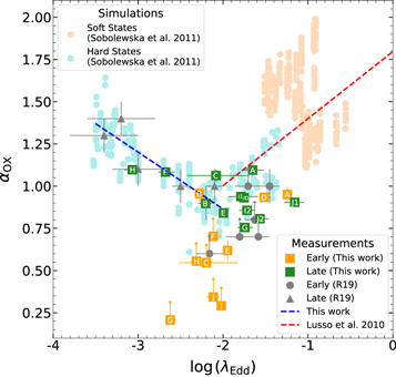
Figure 8. Measured  and
and  of changing-look quasars, including X-ray constraints from ROSAT observations. Orange squares are measurements from ROSAT observations and earliest optical observations (see Table 7). Labels of individual changing-look quasars can be found in column (6) of Table 4 and Table 7. Early measurements of
  and
and  from Ruan et al. (2019a) are denoted by gray circles. Other symbols and lines have the same definitions with Figure 6.
Download figure:
Standard image High-resolution imageTable 7. Measured  and
and  of Changing-look Quasars from ROSAT and SDSS
| Target Name (SDSS) | Optical MJD | X-Ray MJD |

|

| Label |
|---|---|---|---|---|---|
| (1) | (2) | (3) | (4) | (5) | (6) |
| J000904.54-103428.6 | 52141 | 48225 |

|

| A |
| J002311.06+003517.5 | 51900 | 48083 |

|

| B |
| J022556.08+003026.7 | 52200 | 48266 | >0.55 |

| C |
| J132457.29+480241.2 | 52759 | 48214 |

|

| D |
| J160111.25+474509.6 | 52354 | 48083 |

|

| E |
| J164920.79+630431.3 | 51699 | 48083 | >0.70 |

| F |
| J214613.30+000930.8 | 52968 | 48193 | >0.21 |

| G |
| J220537.71-071114.5 | 52468 | 48197 | >0.56 |

| H |
| J225240.37+010958.7 | 52178 | 48292 | >0.29 |

| I |
| J233317.38-002303.5 | 52199 | 48224 | >0.34 |

| J |
Note. (1) Name of CLQs in SDSS. (2) MJD of the optical data, see Table 1 for details. (3) MJD of the X-ray data, see Table 3 for details. (4) Optical/UV–X-ray spectral indices  (
( can be found in Table 2, and
  can be found in Table 6). (5) Logarithmic Eddington ratio, using a bolometric luminosity calculated with only optical data (i.e., Equation (7),
  and
and  can be found in Table 2). (6) Label of orange square data points presented in Figure 8. All error bars denote 1σerrors, and all the lower limits are 3σ.
Download table as: ASCIITypeset image
We also include  and
and  from Ruan et al. (2019a). That work adopts a different bolometric correction in the “early” measurements than our work. To ensure consistency, we recalculate the Eddington ratios of these six “early” measurements, based on their reported
  . These early measurements should be viewed as crude constraints on
  , because the ROSAT and SDSS observations may be separated by up to 13 yr.
Appendix B: Optical Spectra
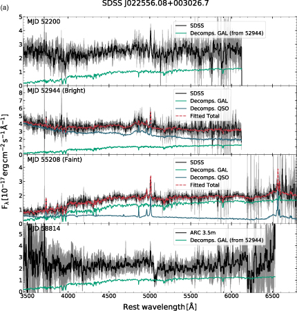
We present spectral decomposition and quasar spectral fitting of other nine CLQs in Figure 9, as described in Section 2.2 and 2.3.
Download figure:
Standard image High-resolution image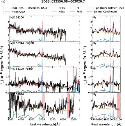
Download figure:
Standard image High-resolution image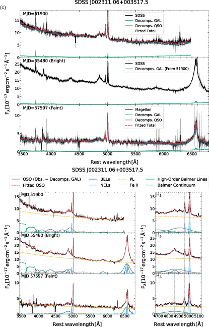
Download figure:
Standard image High-resolution image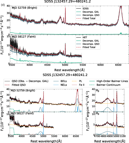
Download figure:
Standard image High-resolution image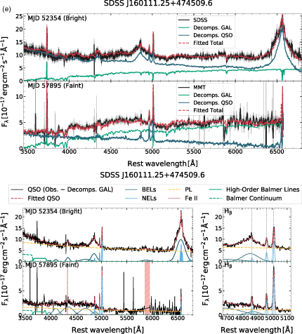
Download figure:
Standard image High-resolution image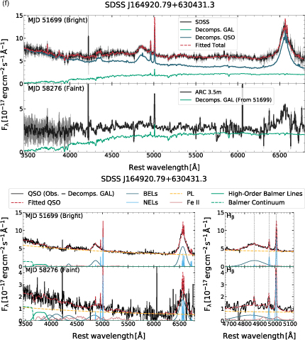
Download figure:
Standard image High-resolution image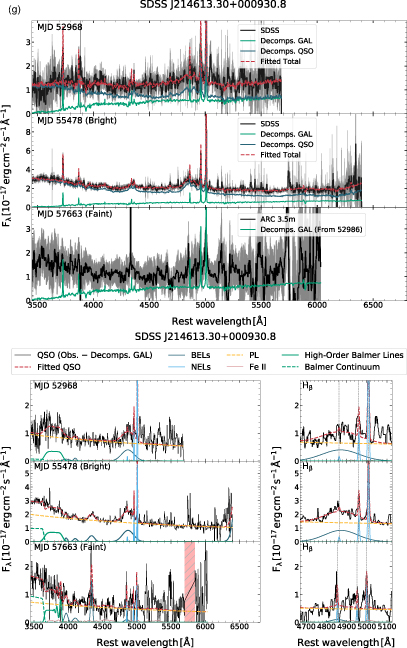
Download figure:
Standard image High-resolution image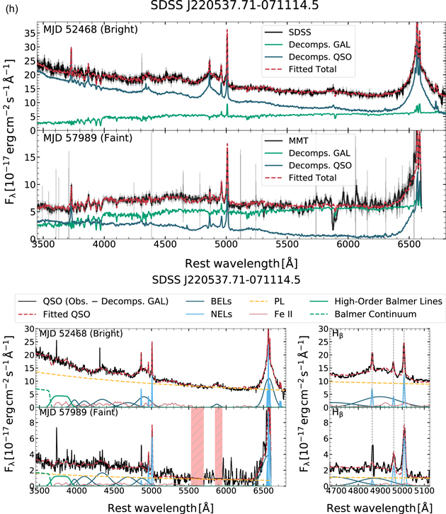
Download figure:
Standard image High-resolution image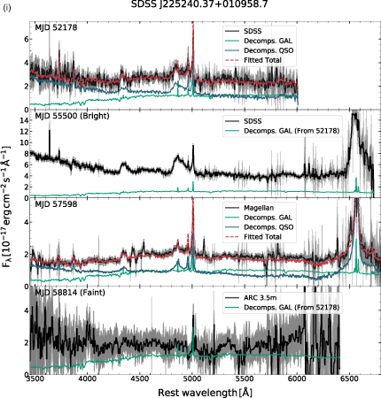
Download figure:
Standard image High-resolution image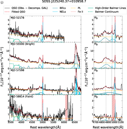
Download figure:
Standard image High-resolution image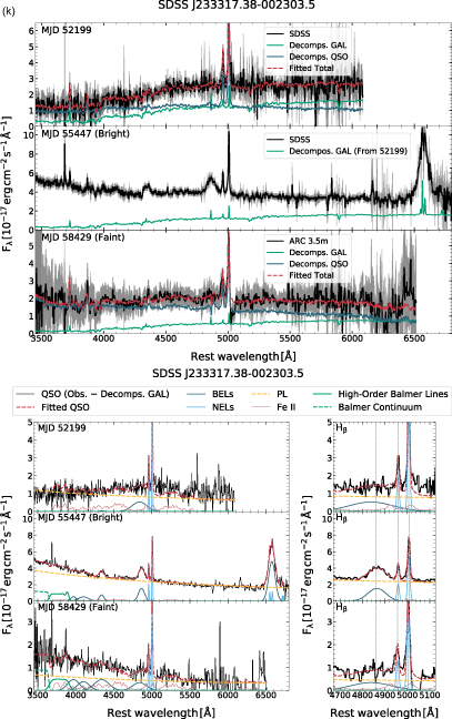
Figure 9. (a) Spectral decomposition for SDSS J022556.08+003026.7. (b) Quasar spectral fitting for SDSS J022556.08+003026.7. (c) Spectral decomposition and the quasar spectral fitting for SDSS J002311.06+003517.5. (d) Spectral decomposition and the quasar spectral fitting for SDSS J132457.29+480241.2. (e) Spectral decomposition and the quasar spectral fitting for SDSS J160111.25+474509.6. (f) Spectral decomposition and the quasar spectral fitting for SDSS J164920.79+630431.3. (g) Spectral decomposition and the quasar spectral fitting for SDSS J214613.30+000930.8. (h) Spectral decomposition and the quasar spectral fitting for SDSS J220537.71-071114.5. (i) Spectral decomposition for SDSS J225240.37+010958.7. (j) Quasar spectral fitting for SDSS J225240.37+010958.7. (k) Spectral decomposition and the quasar spectral fitting for SDSS J233317.38-002303.5. Pink shaded regions are masked when we perform the quasar spectrum fitting.
Download figure:
Standard image High-resolution imageFootnotes
- 11
Though “changing-look” AGN were first introduced to describe AGN that show variable absorption in their X-ray spectra (see Matt et al. 2003), in this work, “changing-look” AGN are only referred to as those AGN that have changed their spectral type based on optical spectroscopy.
- 12
- 13
- 14
- 15
- 16
- 17
We also try fitting the
and relation by using only five data points at in this work, the fitted result (bisector) from BCES is . - 18


