Abstract
Analyses of pulsar timing data have provided evidence for a stochastic gravitational wave background in the nanohertz frequency band. The most plausible source of this background is the superposition of signals from millions of supermassive black hole binaries. The standard statistical techniques used to search for this background and assess its significance make several simplifying assumptions, namely (i) Gaussianity, (ii) isotropy, and most often, (iii) a power-law spectrum. However, a stochastic background from a finite collection of binaries does not exactly satisfy any of these assumptions. To understand the effect of these assumptions, we test standard analysis techniques on a large collection of realistic simulated data sets. The data-set length, observing schedule, and noise levels were chosen to emulate the NANOGrav 15 yr data set. Simulated signals from millions of binaries drawn from models based on the Illustris cosmological hydrodynamical simulation were added to the data. We find that the standard statistical methods perform remarkably well on these simulated data sets, even though their fundamental assumptions are not strictly met. They are able to achieve a confident detection of the background. However, even for a fixed set of astrophysical parameters, different realizations of the universe result in a large variance in the significance and recovered parameters of the background. We also find that the presence of loud individual binaries can bias the spectral recovery of the background if we do not account for them.
Original content from this work may be used under the terms of the Creative Commons Attribution 4.0 licence. Any further distribution of this work must maintain attribution to the author(s) and the title of the work, journal citation and DOI.
1. Introduction
Pulsar timing arrays (PTAs) monitor millisecond pulsars over a timespan of decades. The times of arrival of these radio pulses are sensitive to various physical processes, including variations in the proper distance between the pulsars and the observer due to passing gravitational waves (GWs). PTAs recently reported evidence for a nanohertz stochastic GW background (GWB) in their most recent data sets (Agazie et al. 2023a; Antoniadis et al. 2023a; Reardon et al. 2023; Xu et al. 2023), and their results were shown to be consistent with each other (The International Pulsar Timing Array Collaboration et al. 2023). The most plausible source of this background is a large collection of supermassive black hole binaries (SMBHBs; Agazie et al. 2023b), but other more exotic phenomena can also explain the signal (Afzal et al. 2023).
Several methods have been developed to search for a GWB in PTA data sets. While the GWB is expected to first appear as a common uncorrelated red-noise (CURN) process, the definitive signature of a GWB is considered to be the characteristic Hellings–Downs (HD; Hellings & Downs 1983) angular correlation pattern between pulsars. The most notable frequentist method is the so-called optimal statistic (OS; Chamberlin et al. 2015), which is an unbiased maximum-likelihood estimator of the GWB amplitude based on the cross-correlations between pulsars and the theoretical correlation pattern. It also allows one to define a signal-to-noise ratio (S/N), which is used as a detection statistic. Bayesian methods, on the other hand, marginalize over the parameters of a Fourier-basis Gaussian process that describes the GWB (Lentati et al. 2013; van Haasteren & Vallisneri 2014). This can be constructed either with (HD model) or without (CURN model) HD correlations between pulsars. One can calculate the Bayes factor (BF) between these two models, which is the most important quantity in quantifying the level of Bayesian evidence for a GWB.
As with any statistical data analysis, one needs to make various assumptions when calculating either the OS S/N or the HD versus CURN BF. Most commonly, one assumes that the GWB is (i) Gaussian, (ii) isotropic, or (iii) described by a power-law spectrum 73 . However, if the GWB is produced by a finite number of SMBHBs, none of these assumptions holds exactly (see, e.g., Bécsy et al. 2022). Methods have been developed that relax some of these assumptions. Assumption (iii) is the most often relaxed assumption. It is relaxed either by modeling the spectrum as a two-component so-called broken power-law model, or by allowing the amplitudes of different frequency components to vary freely (see, e.g., Sampson et al. 2015; Taylor et al. 2017; Agazie et al. 2023a, 2023c, K. Gersbach et al. 2023, in preparation, Lamb et al. 2023; Meyers et al. 2023). Some specific searches were also conducted for an anisotropic GWB (Mingarelli et al. 2013; Taylor & Gair 2013; Gair et al. 2015; Romano et al. 2015; Ali-Haï et al. 2020; Taylor et al. 2020; Pol et al. 2022; Agazie et al. 2023d), thus relaxing assumption (ii). One way of relaxing the assumption of Gaussianity is to model the background as a t-process, where the GWB power at each frequency follows a Student t-distribution instead of a Gaussian distribution, thus allowing more flexibility (see Appendix D in Agazie et al. 2023a). While generalized search algorithms like these are available, the flagship results in most GWB searches continue to rely upon these assumptions (see, e.g., Agazie et al. 2023a; Antoniadis et al. 2023a; Reardon et al. 2023). This is in part due to their simplicity, which makes them easier to compute. In addition, it is widely expected that their assumptions are good enough to make them strong and robust methods.
The expectation that models employing these assumptions are capable of detecting GWBs even when these assumptions are broken is based largely on Cornish & Sesana (2013) and Cornish & Sampson (2016). Cornish & Sesana (2013) showed that even a single SMBHB produces HD correlations in an array of isotropically distributed pulsars—showing that we can trade the isotropy of the background for the isotropy of the pulsar array. In Cornish & Sampson (2016), the authors studied both realistic GWBs based on SMBHB population models and also idealized Gaussian isotropic GWBs with a power-law spectrum. They found that the significance with which one can detect these is similar, except for cases with an unrealistically low number of binaries. In this paper, we carry out a similar analysis with a number of improvements.
- 1.We use a more up-to-date SMBHB population model.
- 2.Instead of pulsars with evenly sampled data, we use the actual observation times from the NANOGrav 15 yr data set (Agazie et al. 2023e).
- 3.In addition to white noise, we include pulsar red noise, and we set the level of this noise based on the noise properties found in the NANOGrav 15 yr data set (Agazie et al. 2023c);
- 4.Instead of a simple frequency-domain analysis, we use the actual software used in Agazie et al. (2023a), which works in the time domain and takes covariances with the timing model into account.
Our analysis can also be considered as an extension of the consistency checks carried out in Johnson et al. (2023). There, these analysis pipelines were extensively stress-tested to ensure that they performed properly under the assumption that the data analyzed conform to the models used. We extend the scope to see how these pipelines perform if their assumptions are not met perfectly, as is expected to be the case when analyzing real data. This is a special kind of model mis-specification, where our signal model does not match the data. Understanding the effects of signal model mis-specification, along with noise model mis-specification (Goncharov et al. 2021) and developing consistency checks for our models (Meyers et al. 2023), will be increasingly important as PTAs become progressively more sensitive.
The rest of the paper is organized as follows. In Section 2 we describe our realistic population-based simulated data sets and give more details about the statistical methods employed on them. In Section 3 we present our results, and in Section 4 we provide a brief conclusion and discuss future work.
2. Methods
2.1. Realistic Simulated Data Sets
Our simulated data sets are based on the pulsars and their measured noise properties in the NANOGrav 15 yr data set (Agazie et al. 2023e), following the simulation framework of Pol et al. (2021). We use the libstempo software package, and we simulate data sets with the actual observing times from the real data set. To reduce the data volume, however, we only keep one observation per epoch. We simulate data with the white- and red-noise properties fixed to the maximum a posteriori values inferred from the NANOGrav 15 yr data set (Agazie et al. 2023c).
To simulate the contribution of a realistic GWB, we use an SMBHB population model implemented in the holodeck software package (L. Z. Kelley et al. 2023, in preparation), based on the Illustris cosmological hydrodynamical simulation (Vogelsberger et al. 2014). This model applies a post-processing step to account for small-scale physics not captured by Illustris, uses a phenomenological model to describe binary evolution (for details, see Agazie et al. 2023b), and produces a simulated list of binaries in the universe (Kelley et al. 2017a, 2017b, 2018). To add the contribution of these binaries, we model the brightest 1000 binaries in each frequency bin individually and add the rest as a stochastic background. This was shown to produce results equivalent to a full simulation, but with drastically reduced runtimes (Bécsy et al. 2022). We produce hundreds of realizations of these simulations by drawing new binary populations to account for cosmic variance, and randomizing their extrinsic parameters (sky location, inclination, polarization angle, and phases). We then analyze them with both Bayesian and frequentist statistical methods, which are described in the next sections.
2.2. Bayesian Methods
To carry out a Bayesian statistical analysis of our data sets, we use the following likelihood function (for more details, see, e.g., Equation (7.35) in Taylor 2021):

where δ t are the timing residuals, and C is the noise covariance matrix that includes the effects of both white and red noise and the linearized timing model. The matrix C depends on the parameters describing the noise. In our analysis, we fix the white-noise parameters to their true values. We model the spectrum of the intrinsic pulsar red noise with a power-law model, so that its power spectral density (PSD) in the ith pulsar is
where Ai and γi are the amplitude and the spectral slope of the red noise in the ith pulsar, respectively, and fyr = (yr)−1 is the frequency corresponding to a period of a year. We marginalize over Ai and γi in our analysis. Similarly, we model the timing residuals induced by the GWB as a red-noise process with a power-law spectrum, such that its cross-power spectral density between the ith and jth pulsar is
where Γij is the overlap reduction function (ORF) between the two pulsars. For a GWB, the ORF is given by the HD curve (Hellings & Downs 1983), which introduces correlations between pulsars depending on their angular separation on the sky. Another useful model is the CURN, which assumes Γij = δij , that is, no correlation between pulsars. This model is much more efficient to calculate because C is block diagonal. In practice, the posteriors on AGWB and γGWB are similar between the CURN and HD models. This allows one to sample the simpler CURN model and reweight the posterior samples to obtain fair draws from the HD posterior (for details, see Hourihane et al. 2022). The mean of the weights also serves as a measurement of the BF between the HD and CURN models, which is the primary quantity one needs to measure to claim a detection of the GWB. The variance of the weights can be used to approximate the number of effectively independent samples after reweighting. The ratio of this to the total number of samples defines the reweighting efficiency, which needs to be sufficiently high to obtain reliable results. Only 17 of the 773 realizations we analyzed showed a reweighting efficiency lower than 5%, most of which resulted in only a modest error of the measured BFs, altough the efficiency is low. Thus, the use of the reweighting technique should not have a significant effect on our results.
2.3. Frequentist Methods
While GWB searches usually focus on Bayesian methods, frequentist methods can also be useful, particularly because their computational speed is significantly faster. The most common frequentist method used in searches for a GWB is the so-called OS (Chamberlin et al. 2015), which is an unbiased estimator of the GWB amplitude. It is constructed by maximizing the likelihood of the measured cross-correlation values under the assumption of an ORF and a (typically power-law) PSD model. This results in the estimated GWB amplitude ( ) and the standard deviation of that estimate (σA
). The ratio of these gives the S/N, which can be used as a detection statistic for the presence of a GWB.
) and the standard deviation of that estimate (σA
). The ratio of these gives the S/N, which can be used as a detection statistic for the presence of a GWB.
One disadvantage of the OS is that one needs to know the PSD describing the GWB and the intrinsic red noise of each pulsar, which is not known a priori in a real data set. One can measure the PSD using Bayesian methods, and a point estimate (usually the maximum a posteriori) can be used to calculate the OS. However, this does not take the uncertainty of the measured spectrum into account. To do this, Vigeland et al. (2018) developed the so-called noise-marginalized OS, which calculates the OS for random draws of the spectrum from a Bayesian posterior, thus producing a distribution of OS values. Subsequently, Vallisneri et al. (2023) have also proposed a related method for interpreting the OS in the context of posterior predictive checking.
The OS can also be used to calculate the S/N of processes described by different ORFs. Two commonly calculated ORFs are the monopole and dipole, which could arise, e.g., from systematic clock errors and ephemeris errors, respectively. One limitation of the standard OS is that because these ORFs are usually not orthogonal, processes with less preferred ORFs can still produce high S/N values. To alleviate this problem, Sardesai & Vigeland (2023) developed the so-called multicomponent OS, which can allow multiple processes with different ORFs to fit the data simultaneously. As a result, different processes can be better decoupled. In this study, we calculate S/N values with the noise-marginalized multicomponent OS method to assess the frequentist significance of the GWB, along with monopole- or dipole-correlated processes.
3. Results
To produce robust results, we analyzed 773 different realizations of our simulated 15 yr data set. The median (thick lines) and mean (thin lines) GWB spectra over these realizations are shown in Figure 1, both for all the binaries (solid red lines) and for all except the brightest binaries in each bin (dashed green lines). The shaded region represents amplitudes between the 5th and 95th percentile in each bin. We also show a spectrum with γ = 13/3 as a reference. Note that this has a slope between the median and mean lines for all sources, which give γ = 4.6 and γ = 4.2 in a linear fit to the first five frequency bins, respectively. We can also see that the median spectrum is similar to the mean spectrum when the brightest binary is removed. However, for the total spectrum, the mean spectrum is shallower and follows the expected 13/3 spectral slope better. This is due to the fact that the median is insensitive to outliers, and thus we lose the information about the bright sources.
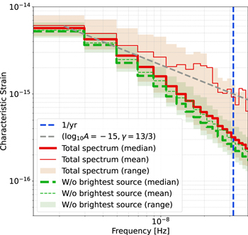
Figure 1. Mean and median GWB spectra over 773 realizations. Also shown is the spectrum after removing the contribution of the brightest binary in each frequency bin. The shaded regions show the range of spectra between the 5th and 95th percentile. We also show a power-law spectrum with a canonical 13/3 slope as a reference.
Download figure:
Standard image High-resolution image3.1. Stochastic Background
We carry out a Bayesian search for a 14-frequency CURN process in each realization, resulting in posterior distributions of the power-law parameters. Based on these, we calculate the median AGWB and γGWB values for each realization. Their distribution is shown in Figure 2 (blue), along with AGWB and γGWB values estimated by a simple least-squares fit to the theoretical spectrum using either the first five (orange) or the first 14 (green) frequency bins. Interestingly, fitting to the first five frequencies gives very similar values to the actual Bayesian CURN analysis, even though that uses the first 14 frequencies. This is due to the fact that the Bayesian analysis is dominated by the first few frequencies, where the signal is strongest. Conversely, a 14-frequency fit to the spectra provides unrealistically accurate measurements, as it does not take the effect of red and white noise into account, the latter of which dominates the GWB signal at higher frequencies. Note that all of these distributions center roughly around the theoretically expected γGWB = 13/3 value and the amplitude to which this population was calibrated. However, they show a significant spread, indicating that the lower γGWB value and higher amplitude found in the NANOGrav 15 yr GWB search (posterior distribution and median values shown by the red contour and dot on Figure 2) is compatible with the binary population in our simulations. Note that this is consistent with the findings of Agazie et al. (2023a), who reported that the NANOGrav results are compatible with an SMBHB interpretation based on a comparison between the recovered AGWB and γGWB values and fits to SMBHB population models. 74 As we can see, the Bayesian spectral analysis of population-based simulated data sets yields similar conclusions. This is not surprising given that we see that a simple fit to the spectrum gives results that are very similar to those of a full analysis.
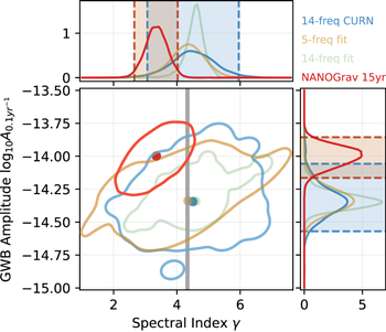
Figure 2. Distribution of recovered median  and γGWB values from a 14-frequency CURN analysis of 773 realizations (blue). Also shown are the values we obtain from a simple least-squares fit to the first five (orange) and first 14 (green) frequency bins of the simulated spectra, and the parameters reported in Agazie et al. (2023a) based on the NANOGrav 15 yr data set (red). The contours represent 99.7% levels (3σ), and the dots show the medians. The one-dimensional marginal distributions are also shown, and the 95.4% intervals (2σ) are highlighted for some of the distributions. While the NANOGrav results show a γGWB value lower than the 13/3 value expected from circular GW-driven GWB (gray), it is well within the spread of γGWB values found in our simulated data sets.
Download figure:
Standard image High-resolution imageFor each realization, we also produce HD posteriors using the reweighting method (Hourihane et al. 2022). We calculate the BF between the HD and CURN models, which are shown as the blue histogram in Figure 3. Note the large variance of the BF, even though we fixed the astrophysical parameters of the simulation (more than eight orders of magnitude between the lowest and highest BF). To understand the source of this variance, it is worth looking at the recovered BFs as a function of the amplitude of the GWB. Figure 4 shows the BFs as a function of  , i.e., the amplitude of the GWB referenced at a frequency of 0.1yr−1 instead of the usual 1yr−1. We use this reference point because the amplitude there is less covariant with γGWB. We can see that while the BF is correlated with the amplitude, we see significant scatter in it even at a given fixed amplitude. Thus, even for universes described by the same astrophysics and a GWB with the same amplitude, the recovered BF shows a significant variance. This is consistent with previous findings on both astrophysical and simple power-law backgrounds (Cornish & Sampson 2016; Hourihane et al. 2022). Thus, this is a generic property of any stochastic background and is not specific for astrophysical backgrounds.
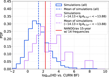
Figure 3. Distribution of HD vs. CURN BFs for all 773 realizations (blue) and for 14 realizations with a recovered amplitude consistent with the amplitude recovered in the NANOGrav 15 yr analysis at the 90% confidence level (purple). Also shown are the means of these distributions (dashed vertical lines) and the BF reported in Agazie et al. (2023a) based on the NANOGrav 15 yr data set (red). While this particular astrophysical model predicts amplitudes and BFs that tend to be lower than the one found in the NANOGrav 15 yr data set, if we select a subset of these that produce a consistent amplitude, they also show good consistency in terms of BF.
Download figure:
Standard image High-resolution image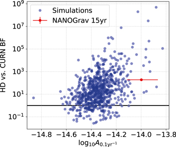
Figure 4. HD vs. CURN BFs as a function of the recovered GWB amplitude referenced at f = 0.1yr−1 (blue dots). While there is a correlation between the amplitude and the BF, the BFs show significant variance even at a given amplitude. Also shown is the BF and amplitude reported in Agazie et al. (2023a) based on the NANOGrav 15 yr data set (red).
Download figure:
Standard image High-resolution imageFigure 3 also shows the histogram of BFs for realizations that show an amplitude that is consistent at the 90% level with that reported in the NANOGrav 15 yr GWB search (Agazie et al. 2023a), along with the actual measured BF in that search. We can see that the simulations show a scatter of about four orders of magnitude even in this narrow amplitude range, but they predict BFs that are roughly consistent with the real data. Note that this is not a rigorous consistency check of the 15 yr results with the astrophysical predictions because our astrophysical models tend to produce a lower amplitude than that found in the 15 yr data set. Thus, the mean of our simulations produces a lower amplitude and lower BF than found in the 15 yr data. However, when we filter out only the realizations that produce an amplitude close to the one found in the real data, we find that the BFs are consistent with that measured on real data. This shows that our simplified analysis methods are capable of detecting the GWB with the significance reported in (Agazie et al. 2023a), even if the GWB comes from a finite number of binaries.
We also calculate the noise-marginalized multicomponent optimal statistic for all realizations. Figure 5 shows the distribution of the mean monopole, dipole, and HD S/Ns, along with the HD versus CURN BFs and  . We also indicate the values found in the NANOGrav 15 yr data set in Figure 5 (red markers). Note that these are all roughly consistent with our simulations. The black lines represent zero S/Ns and BFs. Note that, as expected, both monopole and dipole S/N values are centered around zero, while the HD S/N distribution is offset toward positive values.
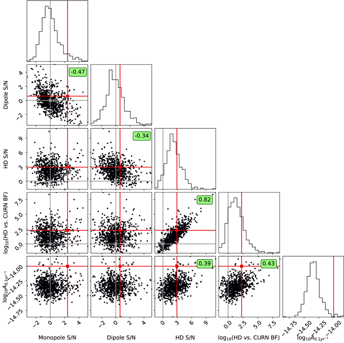
Figure 5. Distribution of mean OS S/Ns, HD vs. CURN BFs, and recovered GWB amplitude referenced at f = 0.1yr−1. The gray lines represent zero S/Ns and unit BFs, and the red lines represent the values reported in Agazie et al. (2023a) based on the NANOGrav 15 yr data set. We also indicate the Pearson correlation coefficient for every pair where the associated p-value is below 10−3.
Download figure:
Standard image High-resolution imageWe can see some interesting correlations between the values shown in Figure 5. To quantify them, we calculate the Pearson correlation coefficient (r) for each parameter pair and show them in the figure where the correlation is significant (p-value <10−3). The strongest correlation of r = 0.82 can be observed between HD S/N and HD versus CURN BF. This is reassuring because they are both meant to quantify the significance of the presence of HD cross-correlations in the data. In fact, both Pol et al. (2021) and Vallisneri et al. (2023) presented an approximate mapping between these two quantities. Both the HD S/N and HD versus CURN BF values are also correlated with  , with r = 0.39 and r = 0.43, respectively. These relatively low correlation values are in line with our finding above that a large variation remains in the detection statistics even at a fixed amplitude. The fact that the amplitude is more strongly correlated with the BF than with the HD S/N can potentially be explained by the fact that the Bayesian analysis uses both autocorrelation and cross-correlation information, while the OS solely relies on cross-correlations. Additionally, both monopole and HD S/N are anticorrelated with the dipole S/N. However, there seems to be no correlation between the HD and monopole S/N.
3.2. Individual Binaries
We investigate the detection prospects of individual binaries (also called continuous waves; CW) and how they relate to background properties by following Bécsy et al. (2022): We calculate the expected S/N of binaries defined as  , where s is the simulated CW signal, i.e., we calculate the inner product of the waveform with itself. We do so for each binary with randomly assigned extrinsic parameters (sky location, inclination angle, polarization angle, and phases), and we find the binary with the highest S/N in each realization. Figure 6 shows the S/N and GW frequency of that best binary in each realization, along with the
  and γGWB values we find in our CURN analysis. Similarly to Bécsy et al. (2022), we find that the highest-S/N sources tend to be found at moderate frequencies around 2–10 nHz. We find a higher mean S/N, which is not surprising given the inclusion of additional pulsars and updated noise models of NANOGrav 15 yr pulsars.
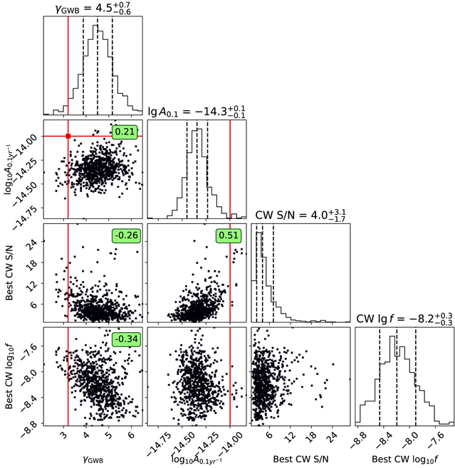
Figure 6. Distribution of GWB spectrum parameters (γGWB,  ) based on a CURN analysis, and S/N and
  of the highest-S/N CW source in each realization. The red lines represent the values reported in Agazie et al. (2023a) based on the NANOGrav 15 yr data set. We also indicate the Pearson correlation coefficient for every pair where the associated p-value is below 10−3.
Download figure:
Standard image High-resolution imageWe calculate the Pearson correlation coefficient (r) for each parameter pair and show it in Figure 6 where the correlation is significant (p-value <10−3). The most significant correlation is shown between the CW S/N and  , with r = 0.51. This can be attributed to the fact that the CURN analysis does not include a CW model, so that if a CW is present, the recovered amplitude is expected to be biased high. We also find a significant anticorrelation between the CW S/N and γGWB (r = − 0.26). This is probably due to the fact that γGWB can be biased low by a significant individual binary at moderate frequencies, as we show below. Finally, the only parameter that correlates with the frequency of the loudest binary is γGWB, showing a negative correlation with r = − 0.34. This can be understood by the fact that the higher the binary frequency, the stronger its potential to bias the GWB slope low.
To further investigate the covariance between individual binaries and the GWB, we analyzed a single realization with the model of an individual binary and CURN (CURN+CW). For this analysis, we used QuickCW (Bécsy et al. 2022, 2023), a software package that builds on the enterprise (Ellis et al. 2019) and enterprise extensions (Taylor et al. 2021) libraries, but uses a custom likelihood calculation and a Markov chain Monte Carlo sampler tailored to the search for individual binaries. We selected this realization randomly under the constraints that it has a CW S/N > 5 and a monopole S/N > 1.5. The former ensured that there is a detectable individual binary in the data, while the latter was motivated by the subdominant monopolar signature found around 4 nHz in the NANOGrav 15 yr data set (Agazie et al. 2023a), which was also identified by the individual binary search carried out using that data set (Agazie et al. 2023f). The selected realization has a monopole S/N of 1.8, a dipole S/N of −1.33, an HD S/N of 2.29, an HD versus CURN BF of 77, a  , a CW S/N of 6.2, and a CW frequency of 9 nHz.
Analyzing this data set with the CURN+CW model, we found that the CW signal was clearly detected, with a CURN+CW versus CURN BF of ∼25. Moreover, the parameter recovery of the CURN process was significantly affected by the inclusion of the CW model. Figure 7 shows the distribution of γGWB and  under the CURN (red), HD (orange), CURN+CW (black), and HD+CW (blue) models. Posteriors with models including HD were produced by reweighting (Hourihane et al. 2022). We can see that in the case of the CURN-only and HD-only models, the unmodeled binary biases the γGWB recovery low compared to the canonical 13/3 value, while the CURN+CW and HD+CW models produce γGWB posteriors centered on values close to 13/3. This is understandable because the CURN model can partially model the CW signal by introducing more power at higher frequencies where the CW is present. This is also consistent with the correlation between γGWB and CW properties we found in Figure 6. While we cannot draw definitive conclusions from a single realization, this result suggests that modeling individual binaries along with the GWB may be crucial for an unbiased spectral characterization of the GWB. We leave a detailed investigation of this problem to a future study.
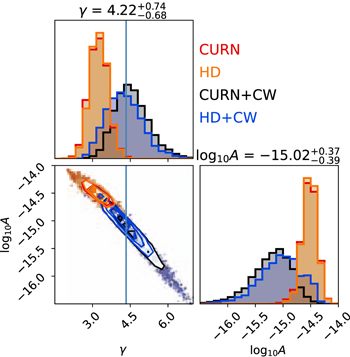
Figure 7. Distribution of GWB parameters under the CURN (red), HD (orange), CURN+CW (black), and HD+CW (blue) models for a particular realization with a clearly detectable binary (S/N = 6.2). Not modeling the CW signal biases the spectral slope low while, when we include it, we recover the expected γ = 13/3 value. Note that in this particular example, the CURN and HD models show very similar posteriors, while the spectral recovery is slightly different between the CURN+CW and HD+CW models.
Download figure:
Standard image High-resolution imageIt is important to note that while the NANOGrav 15 yr analysis recovers a γGWB value lower than 13/3, this does not significantly change with the inclusion of an individual binary model (Agazie et al. 2023f), and the γGWB recovery is instead more affected by the particular noise models employed (Agazie et al. 2023a). This is different from the EPTA DR2 analysis, where the inclusion of an individual binary completely changes the GWB recovery (Antoniadis et al. 2023b). This highlights that both a mis-specified signal model and a noise model can have adverse effects on the parameter estimation.
Note that in this particular realization, the recovered spectra under the CURN and HD models are practically identical (red and orange in Figure 7). This is not particularly surprising because this forms the basis of the reweighting technique (Hourihane et al. 2022). In the presence of an individual binary, the inclusion of correlations does have a small effect on the recovered spectrum (compare the black and blue lines in Figure 7), but the difference is small enough for the reweighting technique to be effective.
In addition, the significance of the individual binary does not change significantly after reweighting. We show the distribution of some individual binary model parameters in Figure 8. The black lines show posteriors from the CURN+CW run, and the blue lines show those that were reweighted to HD+CW. The red lines indicate the true parameters of the signal. In both cases, the binary is clearly detected. The reweighted posterior distributions are similar to the original ones, but are less strongly constrained. We can also see that the recovery of some parameters shows nonnegligible bias. This run is well converged, and QuickCW has been shown to produce unbiased parameter estimates (Agazie et al. 2023f) in CURN+CW simulations. Thus, we suspect that this bias is due to some model mis-specification, e.g., because the background is modeled with a power-law spectrum, or because we assume that only one significant binary is present. In particular, the unmodeled contributions of subdominant binaries at similar frequencies could potentially result in strong biases in some parameters because the sampler tries to adjust the model to fit contributions from more than one binary. In these particular realizations, there are three binaries with frequencies within 1/(2Tobs) ≃ 2 nHz and amplitudes within a factor of three of the loudest binary. This effect is being investigated in a follow-up systematic injection study, where we analyze a large number of realizations under the CURN+CW model. If this bias is indeed the result of the single-binary assumption, an analysis modeling multiple binaries simultaneously could alleviate the problem. An efficient implementation of such an analysis is under development based on an existing multibinary pipeline (BayesHopper; Bécsy & Cornish 2020) and techniques from the efficient single-binary QuickCW algorithm (Bécsy et al. 2022).
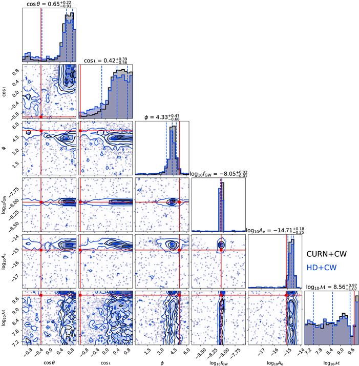
Figure 8. Distribution of the CW parameters for a particular realization from a CURN+CW analysis (black) and those that were reweighted to HD+CW (blue). The red lines represent the true parameter values.
Download figure:
Standard image High-resolution image4. Conclusion and Future Work
We used state-of-the art statistical data analysis techniques to search for a stochastic GW background in realistic simulated data sets. We employed both Bayesian and frequentist techniques to estimate the parameters of the background and assess its significance. Our simulated data sets were produced based on an astrophysical population of SMBHs, and as such, the resulting stochastic backgrounds were anisotropic, non-Gaussian, and had non-power-law spectra. We found that standard analysis techniques were able to detect the characteristic HD correlations in these backgrounds even though they assume isotropic Gaussian power-law backgrounds.
These analyses were also able to correctly characterize the spectrum of these backgrounds most of the time. However, we found that the presence of a strong individual binary can bias the recovered amplitude high and the recovered spectral slope low. We calculated the S/N of the loudest individual binary in each realization and examined how it relates to the background properties.
The fact that standard statistical analysis techniques used by the PTA community can indeed detect the signals from a realistic SMBHB population is reassuring. On the other hand, the possibility that individual binaries can bias the spectral recovery is cause for concern and suggests that joint analyses of individual binaries and the background might become necessary to avoid a biased inference. Future studies investigating the interplay between these two source types will be crucial in ensuring that any astrophysical interpretation is robust. In addition, it will be important to assess the importance of modeling multiple binaries simultaneously. We also plan to investigate the expected level of anisotropy in the stochastic background based on these realistic simulations using methods described, e.g., in Agazie et al. (2023d) and Gardiner et al. (2023). While the results presented in this paper are based on a fixed astrophysical model, investigating the effect of astrophysical parameters on the resulting background and individual binary prospects is also being investigated (Gardiner et al. 2023).
Note that a similar independent analysis was reported concurrently in Valtolina et al. (2023), with results consistent with ours. The analysis was based on simulated data sets resembling the latest data set of the European Pulsar Timing Array. This highlights that our results are robust against the choice of the specific data set on which we base our simulations. One difference between the results is that Valtolina et al. (2023) find that their spectral index recovery is biased high, while we see an unbiased recovery of the spectral index on average (see Figure 2). This is potentially due to the fact that the data set we consider is significantly longer, which allows access to lower frequencies, where the spectrum is less affected by finite-number effects.
Acknowledgments
We appreciate the support of the NSF Physics Frontiers Center Award PFC-1430284 and the NSF Physics Frontiers Center Award PFC-2020265. L.B. acknowledges support from the National Science Foundation under award AST-1909933 and from the Research Corporation for Science Advancement under Cottrell Scholar Award No. 27553. P.R.B. is supported by the Science and Technology Facilities Council, grant No. ST/W000946/1. S.B. gratefully acknowledges the support of a Sloan Fellowship and the support of NSF under award #1815664. M.C. and S.R.T. acknowledge support from NSF AST-2007993. M.C. and N.S.P. were supported by the Vanderbilt Initiative in Data Intensive Astrophysics (VIDA) Fellowship. K.Ch., A.D.J., and M.V. acknowledge support from the Caltech and Jet Propulsion Laboratory President’s and Director’s Research and Development Fund. K.Ch. and A.D.J. acknowledge support from the Sloan Foundation. Support for this work was provided by the NSF through the Grote Reber Fellowship Program administered by Associated Universities, Inc./National Radio Astronomy Observatory. Support for H.T.C. is provided by NASA through the NASA Hubble Fellowship Program grant #HST-HF2-51453.001 awarded by the Space Telescope Science Institute, which is operated by the Association of Universities for Research in Astronomy, Inc., for NASA, under contract NAS5-26555. Pulsar research at UBC is supported by an NSERC Discovery Grant and by CIFAR. K.Cr. is supported by a UBC Four Year Fellowship (6456). M.E.D. acknowledges support from the Naval Research Laboratory by NASA under contract S-15633Y. T.D. and M.T.L. are supported by an NSF Astronomy and Astrophysics Grant (AAG) award number 2009468. E.C.F. is supported by NASA under award number 80GSFC21M0002. G.E.F., S.C.S., and S.J.V. are supported by NSF award PHY-2011772. The Flatiron Institute is supported by the Simons Foundation. S.H. is supported by the National Science Foundation Graduate Research Fellowship under grant No. DGE-1745301. The work of N.La. and X.S. is partly supported by the George and Hannah Bolinger Memorial Fund in the College of Science at Oregon State University. N.La. acknowledges the support from Larry W. Martin and Joyce B. O’Neill Endowed Fellowship in the College of Science at Oregon State University. Part of this research was carried out at the Jet Propulsion Laboratory, California Institute of Technology, under a contract with the National Aeronautics and Space Administration (80NM0018D0004). D.R.L. and M.A.M. are supported by NSF #1458952. M.A.M. is supported by NSF #2009425. C.M.F.M. was supported in part by the National Science Foundation under grant Nos. NSF PHY-1748958 and AST-2106552. A.Mi. is supported by the Deutsche Forschungsgemeinschaft under Germany’s Excellence Strategy—EXC 2121 Quantum Universe—390833306. The Dunlap Institute is funded by an endowment established by the David Dunlap family and the University of Toronto. K.D.O. was supported in part by NSF grant No. 2207267. T.T.P. acknowledges support from the Extragalactic Astrophysics Research Group at Eötvös Loránd University, funded by the Eötvös Loránd Research Network (ELKH), which was used during the development of this research. S.M.R. and I.H.S. are CIFAR Fellows. Portions of this work performed at NRL were supported by ONR 6.1 basic research funding. J.D.R. also acknowledges support from start-up funds from Texas Tech University. J.S. is supported by an NSF Astronomy and Astrophysics Postdoctoral Fellowship under award AST-2202388, and acknowledges previous support by the NSF under award 1847938. S.R.T. acknowledges support from an NSF CAREER award #2146016. C.U. acknowledges support from BGU (Kreitman fellowship), and the Council for Higher Education and Israel Academy of Sciences and Humanities (Excellence fellowship). C.A.W. acknowledges support from CIERA, the Adler Planetarium, and the Brinson Foundation through a CIERA-Adler postdoctoral fellowship. O.Y. is supported by the National Science Foundation Graduate Research Fellowship under grant No. DGE-2139292.
Software: enterprise (Ellis et al. 2019), enterprise_extensions (Taylor et al. 2021), QuickCW (Bécsy et al. 2023), corner (Foreman-Mackey 2016), libstempo (Vallisneri 2020), tempo (Nice et al. 2015), tempo2 (Hobbs et al. 2006), PINT (Luo et al. 2019), matplotlib (Hunter 2007), astropy (Astropy Collaboration et al. 2013; Price-Whelan et al. 2018).
Footnotes
- 73
This also means that we implicitly assume that the signal is stationary.
- 74
Note that Agazie et al. (2023b) carried out much more rigorous analyses that also showed that the GWB is consistent with an SMBHB interpretation.