Abstract
We report the result of our independent image reconstruction of the M87 from the public data of the Event Horizon Telescope Collaborators (EHTC). Our result is different from the image published by the EHTC. Our analysis shows that (a) the structure at 230 GHz is consistent with those of lower-frequency very long baseline interferometry observations, (b) the jet structure is evident at 230 GHz extending from the core to a few milliarcsecond, although the intensity rapidly decreases along the axis, and (c) the “unresolved core” is resolved into three bright features presumably showing an initial jet with a wide opening angle of ∼70°. The ring-like structures of the EHTC can be created not only from the public data but also from the simulated data of a point image. Also, the rings are very sensitive to the field-of-view (FOV) size. The u−v coverage of the Event Horizon Telescope (EHT) lacks ∼ 40 μas fringe spacings. Combining with a very narrow FOV, it created the ∼40 μas ring structure. We conclude that the absence of the jet and the presence of the ring in the EHTC result are both artifacts owing to the narrow FOV setting and the u−v data sampling bias effect of the EHT array. Because the EHTC's simulations only take into account the reproduction of the input image models, and not those of the input noise models, their optimal parameters can enhance the effects of sampling bias and produce artifacts such as the ∼40 μas ring structure, rather than reproducing the correct image.
Original content from this work may be used under the terms of the Creative Commons Attribution 4.0 licence. Any further distribution of this work must maintain attribution to the author(s) and the title of the work, journal citation and DOI.
1. Introduction
Supermassive black holes (SMBHs) at the centers of galaxies often have spectacular jets sharply collimated and extended to intergalactic scale. However, the mechanism of the generation of such jets by the black holes has been an enigma for over a century (Blandford et al. 2019).
The SMBH of the elliptical galaxy M87, the first object of the astrophysical jet discovery (Curtis 1918), is the best place to study the origin of the jet because it has the largest apparent angular size for black holes with strong jets, due to the relatively small distance (16.7 Mpc; Mei et al. 2007) and large mass (6.1 ± 0.4 × 10⁹ M⊙; Gebhardt et al. 2011), which implies that 1 RS = 7 μas. The black hole with the largest apparent angular size, Sgr A*, is present in our galaxy, but unfortunately, it has no jet and its activity is very low in comparison to that of a typical active galactic nucleus (AGN). In addition, it is difficult to obtain high-resolution images of Sgr A* owing to its rapid time variability during very long baseline interferometry (VLBI) observations (Iwata et al. 2020; Miyoshi et al. 2021).
Observations of the core and jet of M87 have been performed in multiple wavelengths, from X-ray to radio (Biretta et al. 1995; Sparks et al. 1996; Biretta et al. 1999; Perlman et al. 1999, 2001; Marshall et al. 2002; Wilson & Yang 2002; Lister & Homan 2005; Perlman & Wilson 2005; Harris et al. 2006; Madrid et al. 2007; Wang & Zhou 2009). Also, high spatial resolution observations using VLBI of the SMBH of M87 have been performed in multiple frequencies up to 86 GHz (Reid et al. 1989; Junor et al. 1999; Lobanov et al. 2003; Ly et al. 2004; Cheung et al. 2007; Kovalev et al. 2007; Ly et al. 2007; Walker et al. 2008; Hada et al. 2011; Hardee & Eilek 2011; Asada & Nakamura 2012; Giroletti et al. 2012; Hada et al. 2013; Nakamura & Asada 2013; Asada et al. 2014; Hada et al. 2016; Mertens et al. 2016; Walker et al. 2016; Britzen et al. 2017; Hada et al. 2017; Kim et al. 2018). Using the “core shift” technique, the distance between the brightness peak of the core and the actual location of the SMBH has been estimated to be from 14 to 23 RS (Hada et al. 2011). Observations with higher spatial resolution at 230 GHz should allow further exploration of the core and jet. Pioneering observations of the Event Horizon Telescope (EHT) 4 were started in 2008 (Doeleman et al. 2008).
In 2017, the Event Horizon Telescope (EHT) attained sufficient sensitivity by including the phased Atacama Large Millimeter/submillimeter Array (ALMA) in the array and equipping all stations with 32 Gbps recording systems. The EHTC reported their findings of a ring-shaped black hole shadow from the observational data (The Event Horizon Telescope Collaboration et al. 2019a, 2019b, 2019c, 2019d, 2019e, 2019f). The ring diameter was approximately 42 μas, which is consistent with that expected from the mass of M87 SMBH (6 × 10⁹ M⊙) obtained using stellar dynamics (Gebhardt et al. 2011). 5 Three research groups have followed up with analyses using EHTC’s open data (Arras et al 2022; Carilli & Thyagarajan 2022; Lockhart & Gralla 2022).
We found three problems in the EHTC imaging results. First, although the EHT’s intrinsic field of view (FOV) is large enough to cover both the core and the jet structure together, no jet structure has been reported by the EHTC. The M87 jet is powerful and has been detected in lower-frequency VLBI observations.
There was no detailed description of the investigation of the jet structure in The Event Horizon Telescope Collaboration et al. (2019a, 2019b, 2019c, 2019d, 2019e, 2019f); in 2017, the EHT array achieved unprecedented sensitivity, so it is not surprising to have strong expectations for detecting new jet structures of M87.
Second, the ring diameter of the EHTC imaging (d = 42 ± 3 μas; The Event Horizon Telescope Collaboration et al. 2019a) coincides with the separation between the main beam and the first sidelobe in the dirty beam (identical to the point-spread function (PSF)) of the EHT u−v coverage for the M87 observations. In the EHTC paper, there is no description of the structure of the dirty beam, such as sidelobes. Misidentification of sidelobes as real images is a common mistake in radio interferometer observations with a small number of stations such as the EHT array. The EHTC do not seem to take such a risk into account (at least it is not clearly mentioned in their paper). There is a possibility that the EHTC ring is a mixture of the real image and the residual sidelobes.
The last problem is the brightness temperature of the ring reported by the EHTC (Tb = 6 × 10⁹ K at most from Figure 3 in The Event Horizon Telescope Collaboration et al. 2019a 6 ), which is significantly lower than that of their previous M87 observations (Tb from 1.23 to 1.42 × 10¹⁰ K; Akiyama et al. 2015) despite having higher spatial resolutions. 7 The 86 GHz Very Long Baseline Array (VLBA; Napier et al. 1993) observations have shown that the core brightness temperature is Tb = 1.8 × 10¹⁰ K (Hada et al. 2016). Kim et al. (2018) also reported the brightness temperature is Tb ∼ (1 − 3) × 1010 K at 86 GHz. The spatial resolutions of both observations are lower than that of EHT (θBEAM > 100 μas), but they show higher brightness temperatures. In any case, it is quite unusual to observe a brightness temperature of less than 1010 K for the M 87 core by VLBI.
In observations of very compact objects, if the spatial resolution is low, the measured brightness temperature could be underestimated because the solid angle of the emission region tends to be overestimated. If the spatial resolution is higher, the measured brightness temperature can be expected to be higher because the solid angle of the emission region can be more accurately identified. The measured brightness temperature increases until the spatial resolution becomes sufficient to resolve the actual structure of the compact object. However, the measured brightness temperature may surely decrease when sufficient spatial resolution is achieved and the fine structure is recognized. The EHTC observations show a ring diameter of about 40 μas, almost the same as the estimated source size in Akiyama et al. (2015). However, since it is a ring structure, the center of the image is darker, so assuming that the flux density is the same, 8 the highest-brightness part in the ring image should show a higher brightness temperature than that indicated by Akiyama et al. (2015).
The lower brightness temperatures and/or flux densities in the images obtained by the EHTC could be the results of insufficient recovery of the data coherence by improper calibrations.
Because of these three problems, we decided to reanalyze the data released by the EHTC. 9 Using the public data released by the EHTC, we succeeded in reconstructing the core and jet structure in M87.
We have resolved the region containing the SMBH in M87 for the first time and found the structure of the core and knot separated by ∼33 μas (550 au or 4.7 RS) on the sky, which shows time variation. This could be the scene of the initial ejection of the jet from the core. We also found a feature to the west, ∼83 μas away from the core. These facts are important for identifying the jet formation mechanism from SMBHs. We need further observations to determine the nature of the features.
We also found emissions along the axis of the jet up to a point a few milliarcsecond from the core, showing that the edges of the jet are brighter, similar to what was observed at low frequencies.
We first describe the observational data released by the EHTC in Section 2, our data calibration and imaging process in Section 3, and our imaging results in Section 4. Then, we investigate how the EHTC ring was created in Section 5. In Appendix A, we show that the EHT array cannot detect any feature whose size is larger than 30 μas. As a supplement to Section 5.2, Appendix B shows the dirty beam (PSF) shapes of the EHT array for the M87 observations in two different types: natural weighting and uniform weighting. Both show the substructure with a scale of ∼40 μas. In Appendix C, we show that the missing spatial Fourier components of ∼40 μas also affect the structure in our CLEAN map.
2. Observational Data
The observational data were recorded on 2017 April 5, 6, 10, and 11. The EHT array consists of seven submillimeter radio telescopes located at five places across the globe, yielding the longest baseline length over 10,000 km (The Event Horizon Telescope Collaboration et al. 2019a). The observational details and the instruments in the series of the EHTC papers (The Event Horizon Telescope Collaboration et al. 2019a, 2019b, 2019c, 2019d, 2019e, 2019f). The raw data archives have not been released by the EHTC yet, but they released the calibrated visibility data with their recipe of the data reduction procedure. We first analyzed the released EHT data sets of M87 using the standard VLBI data calibration procedure and imaging methods without referring to their data procedure. The data are time-averaged into 10 sec bins and are stored into 2 Intermediate Frequency (IF) channels. According to the header of the public FITS data, the Frequency bandwidth is 1.856 GHz in each IF. Because of the removal of data of the strong calibrator source (3C 279), we could not perform the fringe search to correct the errors of station positions, clock parameters, and the receiving band-path calibration by ourselves. Therefore, our independent calibration was limited to the self-calibration method.
We checked the details of the data and noticed that the visibility values of the RR-channel and LL-channel are exactly the same. The headers of the EHTC open FITS data files contain two data columns labeled “RR” and “LL,” respectively; the FITS format data does indeed contain data columns labeled RR and LL. We checked all the original public FITS data sets (there are 8 sets) and confirmed that the data in the RR and LL columns are the same in all the data sets; there are a total of 51119 pairs of RR and LL, and all the pairs have exactly the same real, imaginary, and weight values.
We found in a document of the EHTC the following description 10 : The data are time-averaged over 10 s and frequency averaged over all 32 intermediate frequencies (IFs). All polarization information is explicitly removed. To make the resulting “uvfits” files compatible with popular VLBI software packages, the circularly polarized cross-hand visibilities “RL” and “LR” are set to zero along with their errors, while parallel-hands “RR” and “LL” are both set to an estimated Stokes *I* value. Measurement errors for “RR” and “LL” are each set to sqrt(2) times the statistical errors for Stokes *I*. In other words, the open data in the EHTC FITS format are not the visibility of either polarization, but the Stokes I, Vij,I = (Vij,RR + Vij,LL )/2, (The Event Horizon Telescope Collaboration et al. 2019c), and the above-calculated values are stored in the columns of RR and LL. This information is not included in the attached tables or files of the FITS data. For this, the FITS format for intensity data should have been used instead of the dual polarization data. Also, it means that the corrections made between the correlator output and the open data cannot be independently verified.
EHTC’s open data integrates the wide frequency band of 1.86 GHz into a single channel. Such wideband integration is extremely rare and unsuitable for public data because it results in loss of information over a wide field in the data due to the bandwidth smearing effect. The effect is similar to the peripheral light fall-off of optical camera lenses. Visibility data integrated in the frequency direction reduces the sensitivity in peripheral vision. This phenomenon occurs because originally independent (u, v) points are integrated in frequency domain. The farther away from the center of the FOV (phase center), the larger the size of the PSF and lower the peak; the detection sensitivity in the peripheral vision becomes worse (Thompson et al. 2017 ; Bridle & Schwab 1989; Bridle et al. 1999).
Due to the bandwidth smearing effect, the peak of the PFS away from the phase center has suffered attenuation as shown in Figure 1. In the case of the EHTC open data, the ratios of peak heights relative to that at the phase center are ∼50% at a radius of 5 mas, and ∼27% at a radius of 10 mas. Even at a radius of 20 mas from the center, the ratio is ∼14%. If a component of sufficient intensity is present at even a far away position from the center, it will be detected. We did not abandon such a possibility and set a wide field for imaging as explained in Section 3.
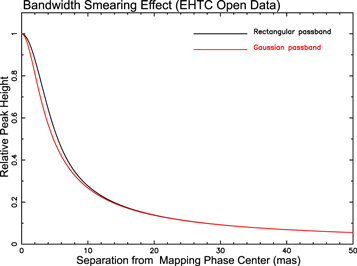
Figure 1. The bandwidth smearing effect calculated explicitly for the EHTC open data by following Equations (75) and (76) of Section 6 in Thompson et al. (2017). Adapted synthesized beam size is θb = 21.06 μas, which is the geometric mean of major and minor axes of the beam shapes of the four observing days shown in Table 1 of The Event Horizon Telescope Collaboration et al. (2019d). We substituted Δν = 1.856 GHz for the bandwidth and ν0 = 229.071 GHz for the observing frequency.
Download figure:
Standard image High-resolution imageThe coherence time of the obtained data has a significant impact on the data analysis and imaging results; the EHTC shows the atmospheric coherence time for all observations in the 2017 campaign (The Event Horizon Telescope Collaboration et al. 2019b), but not for those limited to the M87 observations only. Therefore, we used the AIPS task COHER to check the coherence time of the visibility data. Here, the coherence time is defined as the time when the amplitude becomes 1/e ∼ 0.36 by vector averaging. The task COHER cannot identify the reasons for the coherence loss. In any case, the calculated coherence time represents the total amount of coherence loss that the data has suffered. The coherence time Tcor = 0.45 ± 0.7 minutes was obtained from the entire data set (average of all baselines). However, the coherence time was not constant; the data from the first two days showed Tcor = 0.54 ± 0.91 minutes, and the data from the last two days showed Tcor = 0.35 ± 0.36 minutes. We took it as significant that 39% of the total data showed Tcor ∼0.167 minutes (∼10 s). Without any kind of correct calibrations, we do not expect to improve the signal-to-noise ratio (S/N) by long time integration. We decided that no meaningful solution could be obtained by increasing the integration time (solution interval, hereafter SOLINT) in self-calibration. Therefore, we always set SOLINT to 0.15 minutes when performing self-calibration.
We used both data channels in their original form. We found that our calibrations of the EHT data sets can be significantly improved and also obtained an improved solution for calibrations using the hybrid mapping method (Pearson & Readhead 1984; Readhead & Wilkinson 1978; Schwab 1980). The observations were performed over four days. We succeeded in increasing the sensitivity by integrating two days’ data or all of them.
3. Our Data Calibration and Imaging
In this section, we report on the procedures and results of data calibration and imaging. We used standard methods of VLBI data analysis for sources with unknown structures. In Section 3.1, we describe the hybrid mapping procedures used in this study. Section 3.2 describes how we identified the second feature from the first map, and Section 3.3 describes the process that followed. In Section 3.4, we present our final images. In Section 3.5, we present a solution for self-calibration of both amplitude and phase, using the final image as a model to determine the quality of the EHT public data.
3.1. Hybrid Mapping Process
In the analysis of VLBI data, the hybrid mapping method is widely used to obtain a calibration solution for the data and to reconstruct the brightness distribution. Hybrid mapping, which consists of repeatedly assuming one image model, performing self-calibration, obtaining a trial solution for calibration, and improving the image model for the next self-calibration, is the only method that is reliable for the precise calibration of VLBI data (Pearson & Readhead 1984; Readhead & Wilkinson 1978; Schwab 1980). VLBI systems are not so stable in phase and amplitude as compared to those of connected radio interferometers. In addition, millimeter- and submillimeter-wave observations are strongly affected by atmospheric variations. Therefore, the hybrid mapping method is becoming more and more important in the calibration of high-frequency VLBI data such as the EHT observations. We performed a standard hybrid mapping process using the tasks CALIB and IMAGR in AIPS (the NRAO Astronomical Image Processing System, 11 Greisen 2003).
3.2. The First Step in Hybrid Mapping Process
3.2.1. Solutions of Self-calibration Using a Point-source Model
As a first step in this process, a single point source (located at the origin) was used as the first image model to obtain a solution for the visibility phase calibration from the self-calibration. The parameters used for the task CALIB are listed in Table 1.
Table 1. Parameters of CALIB for the First Self-calibration
| Parameters | |
|---|---|
| SOLTYPE | “L1” |
| SOLMODE | “P” (phase only) |
| SMODEL | 1,0 (1 Jy single point) |
| REFANT | 1 (ALMA) |
| SOLINT (solution interval) | 0.15 (minute) |
| APARM(1) | 1 |
| APARM(7) (S/N cutoff) | 3 |
Download table as: ASCIITypeset image
As mentioned in Section 2, the coherence time of EHT public data is very short. The solution interval (SOLINT) was set to 0.15 minutes. We set the S/N cutoff = 3 for safety. This S/N cutoff value is larger than what many researchers use in the end. Solutions that did not meet the criteria (S/N cutoff) were flagged and abandoned.
Figure 2 shows the phase solution for the first step. Because phase is a relative quantity, the phase of the ALMA station (AA) is used here as a reference. For all stations, the nonzero and time-varying phase values were calculated by self-calibration. The four stations, APEX (AP), The Submillimeter Telescope at the Arizona Radio Observatory (SMT, hereafter AZ), Large Millimeter Telescope in México (LM), and Pico Veleta (PV), always show the same respective trends over the four days of observations, suggesting that there are errors in station positions (a sinusoidal curve with a period of one sidereal day is observed at all stations when there is an error in the position of the observed object).
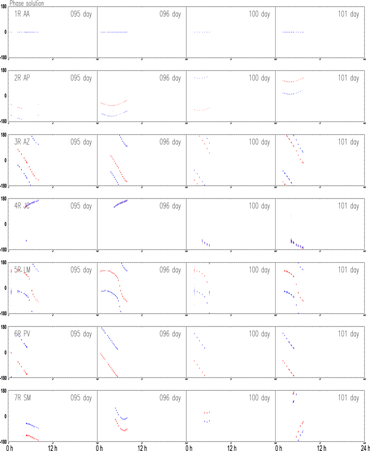
Figure 2. Initial phase (only) solutions obtained by self-calibration using one-point model. The red dots are the solutions for IF 1 data, and the blue dots are those for IF 2 data. The solution for L (left-handed circular) polarization is not plotted here; the visibility data for LL is exactly the same as for RR, so the solution for L is the same as the solution for R in the figure.
Download figure:
Standard image High-resolution imageAnother feature is the phase difference that occurs between IF1 and IF2, which is almost fixed for all stations except James Clerk Maxwell telescope (JCMT, hereafter JC) and AA (phase reference station), respectively.
If the EHT public data were sufficiently calibrated, the above two phenomena should not appear. In conclusion, the “calibrated” data published by the EHTC is not yet sufficiently calibrated. In order to obtain reliable images, the EHT’s public data needs to be further calibrated.
3.2.2. The First CLEAN Map
Figure 3 shows the CLEAN (Clark 1980; Högbom 1974) image obtained from the data after applying the first phase calibration solution shown in Figure 2. The parameters of the imaging of IMAGR are shown in Table 2. (In all figures showing the imaging results, the x-axis indicates relative R.A. and the y-axis relative decl.) The purpose of this imaging is to find the second brightest component following the central brightest peak. As will be explained in Section 5.1, despite the fact that the EHTC has utilized a large number of stations, the u−v coverage of the EHT array is formed by only 7 stations, or actually 5 stations if we exclude the very short baselines. The synthesized beam (dirty beam) of the EHT is not so sharp as those of multielement interferometers such as ALMA and Very Large Array (VLA). It is not easy to find the complex brightness distribution of the observed sources from a tentative map composed of such a scattered dirty beam (PSF). (We show the dirty beam and dirty map in Figures 20 and 21.) Therefore, we performed CLEAN, specified by the parameters shown in Table 2. This method is effective when the structure of the observed source is not point symmetric. We set the loop gain (GAIN) to 1.0 and extracted all of the brightest peak from the dirty map in the first CLEAN subtraction. Next, this component was replaced by a sharp Gaussian restoring beam and combined with the brightness distribution of the remaining dirty map. The image in Figure 3 was created in this way.
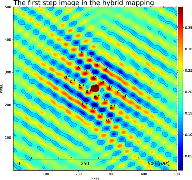
Figure 3. First step image of our hybrid mapping process. The restored beam size is about 20 μas, and the center 600 μas square of the map is magnified. Contour lines are drawn at every 20% level of the peak brightness of 3.981 × 10⁻¹ (arbitrary units are used in the figure, not Jy beam−1). One pixel corresponds to 1.22011 μas.
Download figure:
Standard image High-resolution imageTable 2. Parameters of IMAGR for the First Trial Imaging
| Parameters | |
|---|---|
| DOCALIB | 2 |
| CELLSIZE | 1.22011 × 10⁻⁶, 1.22011 × 10⁻⁶ (arcsec) |
| FLDSIZE | 8192, 8192 (pix) |
| ROBUST | 0 |
| NITER | 1 |
| GAIN | 1.0 |
Download table as: ASCIITypeset image
This has the effect of removing the bright but scattered PSF shape of the brightest point that dominates the dirty map, and clarifying the presence of the second brightest component in the image. Note that if the data is not properly calibrated and the actual PSF corresponding to a point source differs from the theoretically calculated PSF shape, the brightness distribution caused by the brightest point may remain in the afterimage. However, such remaining brightness distribution also shows a point-symmetric structure with respect to the location of the brightest point (practically the same location as the center of the map), and does not contribute to the asymmetric structure of the image. Therefore, if there is an asymmetric structure in the image, it is not related to the brightest component, but is due to another bright point source. So, by searching for the asymmetric structure, we can find the second component of the observed source.
This image (Figure 3 shows its central 600 μas square) has a nearly point-symmetric structure with respect to the center of the map. The overall feature is a series of multiple ridges in the PA = 55° direction. This structure is due to the nonuniformity of the u−v coverage. In addition to the central P, there are several other bright features. The peak brightness of these features is shown in Table 3. Features a, b, c, d, e, f, g, h, i, j, and k have corresponding features located at their symmetry points (denoted as a*, b*, c*, d*, e*, f*, g*, h*, i*, j*, and k*). Curiously, the features located in the upper right from the center are always brighter than their counterparts located in the lower left, i.e., the brightness ratio is greater than one. This may indicate the existence of a large-scale asymmetric brightness distribution in the observed object, extending from the center to the upper right. This is roughly consistent with the M87 jet propagation direction PA = −72° (Walker et al. 2018). Examining the brightness ratio of each pair, we find that the pair c & c* (ratio = 1.146) is the largest, followed by the pair a & a* (ratio = 1.122). Regarding the absolute value of brightness, the brightness of a (2.396 × 10⁻² Jy Beam−1) is larger than that of c (1.982 × 10⁻² Jy Beam−1). In addition, there is a ridge extending from the central bright point (P) toward feature a. The direction of this ridge (PA = −45°) is completely different from the direction of multiple ridges seen in the entire image, and no other ridge shows the same direction. Based on these characteristics, we decided to continue the hybrid mapping by adopting two points for the next image model. In other words, we chose to use a model with a point at each of the two locations, the center and the location of feature a.
Table 3. Peak Brightness of the Features That Appeared in the First Step Image
| Name | Brightness (Jy beam−1) | Name | Brightness (Jy beam−1) | Ratio | Order |
|---|---|---|---|---|---|
| P | 8.736 × 10⁻² | ||||
| a | 2.396 × 10⁻² | a* | 2.136 × 10⁻² | 1.122 | 2 |
| b | 2.438 × 10⁻² | b* | 2.187 × 10⁻² | 1.115 | 3 |
| c | 1.982 × 10⁻² | c* | 1.729 × 10⁻² | 1.146 | 1 |
| d | 2.099 × 10⁻² | d* | 1.889 × 10⁻² | 1.111 | 4 |
| e | 2.780 × 10⁻² | e* | 2.534 × 10⁻² | 1.097 | 5 |
| f | 2.420 × 10⁻² | f* | 2.257 × 10⁻² | 1.072 | 7 |
| g | 2.368 × 10⁻² | g* | 2.205 × 10⁻² | 1.074 | 6 |
| h | 2.334 × 10⁻² | h* | 2.282 × 10⁻² | 1.023 | 9 |
| i | 2.364 × 10⁻² | i* | 2.337 × 10⁻² | 1.012 | 10 |
| j | 2.475 × 10⁻² | j* | 2.404 × 10⁻² | 1.030 | 8 |
| k | 2.328 × 10⁻² | k* | 2.319 × 10⁻² | 1.004 | 11 |
Note. The 11 features near the center are shown. P is the peak in the center that was replaced by the restoring beam. Features other than P are as shown in the brightness distribution of the residual dirty map.
Download table as: ASCIITypeset image
3.3. Our Hybrid Mapping Process
After obtaining the image models for the two points, more than 100 iterations, including trials and errors, were performed in the hybrid mapping process. Most of the CLEAN images were run with the parameters listed in Table 4.
Table 4. Typical Parameters of IMAGR for Our Hybrid Mapping Process
| Parameters | |
|---|---|
| ANTENNAS | 0 (all) |
| DOCALIB | 2 |
| CELLSIZE | 1.5 × 10⁻⁶, 1.5 × 10⁻⁶ (arcsec) |
| UVRANGE | 0, 0 (no limit) |
| FLDSIZE | 16384, 16384 (pix) |
| ROBUST | 0 |
| NITER | 40000 |
| GAIN | 0.05 or 0.005 |
| FLUX | −1.0 (Jy) |
| BMAJ, BMIN | 0.00002, 0.0002, and 0 (arcsec) |
| BPA | 0 (°) |
| RASHIFT | −9.25 × 10⁻³ (arcsec) |
| DECSHIFT | 8.15 × 10⁻³ (arcsec) |
| NBOXES | 8 |
| BOX(1) | −1, 912, 1329, 2185 (pix) |
| BOX(2) | −1, 820, 2049, 2729 (pix) |
| BOX(3) | −1, 912, 3105, 3129 (pix) |
| BOX(4) | −1, 1184, 4481, 3689 (pix) |
| BOX(5) | −1, 1792, 6321, 4473 (pix) |
| BOX(6) | −1, 2448, 8753, 5673 (pix) |
| BOX(7) | −1, 2848, 11537, 7001 (pix) |
| BOX(8) | −1, 2800, 13377, 7833 (pix) |
Note. The imaging area is 24.576 mas square, but it is limited by the BOX setting. “Flux = −1.0” means that the terminating condition of CLEAN subtraction is the first occurrence of a negative maximum value.
Download table as: ASCIITypeset image
As described in The Event Horizon Telescope Collaboration et al. (2019d), care must be taken in the choice of FOV, as incorrect restrictions will result in incorrect image structures. Considering the well-known structure of M87, we restricted the imaging region by eight BOXes where emission could be detected. For the self-calibration, the selected CLEAN components were used as the next imaging model, and the parameters in Table 1 were used. By repeating the phase-only self-calibration in this way, we were able to find better images and calibration solutions. This is because the method of simultaneously solving the amplitude solution with hybrid mapping has the risk of going in the wrong direction. Self-calibration of phase-only can be done with a certain degree of safety. Even if the wrong model is used and a completely wrong solution is obtained, the closed phase is automatically preserved, and convergence to a completely wrong image can usually be avoided. On the other hand, the amplitude solution from self-calibration can be infinitely large or small for a wrong image model. It is safe to try the self-calibration of the amplitude solution after a correct image model is obtained from the phase self-calibration.
3.4. Our Final Image
In the latter half of the imaging process, we selected several candidates for the final image by comparing the difference in the closure phase between the image and the real data. Furthermore, we created several image models using the CLEAN components of the candidate images to find the best image with the minimum closure residuals. Since we found that the source structure shows time variation, we divided the data into the data of the first two days and the data of the last two days. As a result, we obtained the best images as shown in Figure 4. The data from the first two days was a composite of seven raw CLEAN maps, and the data from the last two days was a composite of nine raw CLEAN maps. Both consist of CLEAN components only. In the images of the first two days, adjacent CLEAN components within 2 μas are merged into one component. In the images of the last two days, adjacent CLEAN components within 5 μas are merged into one component.
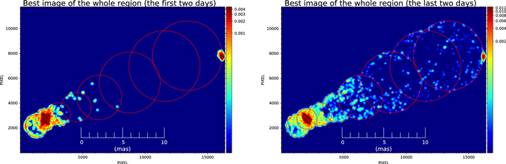
Figure 4. The best images obtained from the analysis. The left panel shows the best image for the data of the first two days. The right panel shows the best image for the data of the last two days. In both images, the grouped-CLEAN components are convolved with a circular Gaussian restoring beam of HPBW = 200 μas. A logarithmic pseudo-color is used to express the large differences in brightness distribution (arbitrary unit). The eight red circles indicate the BOX area used. The bright spot seen on the right (west) edge is not the real brightness distributions (see the content in Section 3.4).
Download figure:
Standard image High-resolution imageSince the eight BOXes cover a large area, the resulting CLEAN component contains three types of emission: real emission, associated diffraction (sidelobes), and false acquisitions. For example, the bright emission on the right edge is not real. Such unreal bright spots often appear when the VLBI data is analyzed and imaged. When such unreal brightness appears, there may actually be strong emissions outside the BOXes. We produced a large image (30 arcsec FOV) using very short baseline (SM-JC and AA-AP) visibility data, but could not detect any new strong features.
To get a more complete image, we need to select only the real ones from these CLEAN components and perform CLEAN imaging again with each narrow BOX to cover the selected ones. However, since our data did not have enough u−v coverage and quality to select the correct ones among the CLEAN components, we gave up the task of extracting the CLEAN components this time. Nevertheless, the quality of the final image does not seem to be too bad. The closure residuals of the resulting image show a small variance comparable to the EHTC ring image. The residual of our map for the first two days of data is −4°.90 ± 37°.93 (the residual of the EHTC ring is −0°.73 ± 45°.33), and the residual of our map for the last two days of data is 1°.79 ± 42°.11 (the residual of the EHTC ring is 4°.22 ± 45°.74). Here, we integrated the 5 minutes data points and calculated the closure phase of all triangles. For more information on closure phase residuals, see Section 4.3.3.
The EHTC ring images for comparison were generated using the EHTC-DIFMAP pipeline. It should be emphasized that the final image clearly contains an unrealistic CLEAN component, but still shows the same level of closure phase residuals as the image of the EHTC ring.
We also used this final image model to attempt self-calibration of the amplitude and phase for the solution, performed CLEAN, and obtained new images. However, the residuals of the closure phase in the new image were not improved. Therefore, we terminated the hybrid mapping without amplitude calibration. The images shown in Figure 4 are our best final images. The two upper panels in Figure 7 and the panels in Figure 10 are partial extracts from the final images. Figure 8 shows the full image of the last two days of data.
3.5. Solutions of Self-calibration Both Amplitude and Phase Using a Final Image Model
Here we show the solutions of the self-calibration for both amplitude and phase using one of the final images, although we did not apply it to the data calibration. The reason we dare to show the unused solutions here is that we believe this study provides insight into the quality of EHT public data and the reliability of our images. We performed our self-calibration using CALIB in the AIPS task in “A&P” mode with the image (CLEAN components). Other parameters of CALIB are the same as in the first self-calibration (Table 1). Figures 5 and 6 show the self-calibration solutions (the total amount of solutions to be applied for data calibration).
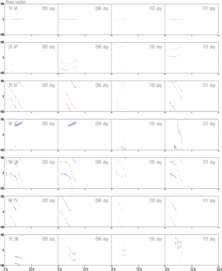
Figure 5. Phase solutions obtained from self-calibration with A&P mode using CALIB in AIPS. As the image model, all of the grouped-CLEAN components of the last two days’ image were used. The red points show the solutions for IF 1 data; the blue ones show those for IF 2 data.
Download figure:
Standard image High-resolution imageFigure 5 shows the phase solution. Compared to the initial phase solution shown in Figure 2, there is no significant change in the overall structure. This can be attributed to the fact that the brightness distribution of the observed source is concentrated in the center and does not deviate significantly from the self-calibration solution assuming a single point source. However, there are offsets in the phase changes of JC, LM, PV, and the Submillimeter Array in Hawaii (SM) stations. In addition, the phases of the two stations in Hawaii, JC and SM, show a larger phase dispersion than the solution of self-calibration assuming a point source on the 100 and 101 days’ data. Although small in comparison, the phases of JC and SM on 95 and 96 days’ data also show phase scatters on the same hours.
The amplitude solution is shown in Figure 6. In general, the errors in amplitude are due to noise in the atmosphere and in the receiving system. In addition, the changes in aperture efficiency depending on the elevation angle of antenna often cause systematic errors in amplitude. These effects can be measured by an auxiliary method.
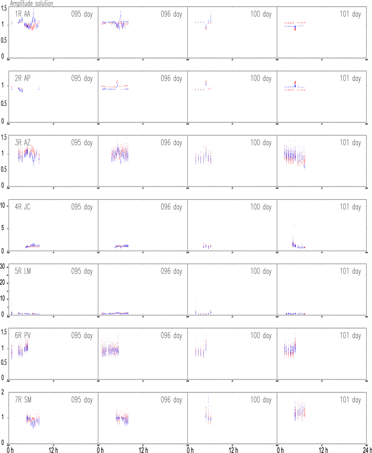
Figure 6. Amplitude solutions obtained from self-calibration with A&P mode using CALIB in AIPS. As the image model, all of the grouped-CLEAN components of the last two days’ image were used. The red points show the solutions for IF 1 data; the blue ones show those for IF 2 data.
Download figure:
Standard image High-resolution imageFor the large aperture antennas, gain loss due to offset tracking of the target source from the narrow main beam angle may occur, which is difficult to calibrate.
Furthermore, coherency (phase stability) loss is observed due to the variations in station clocks and atmospheric variations, which are more difficult to measure correctly than other error factors.
Amplitude solutions for AA, AP, PV, and SM stations are within 50% fluctuation (∼1.0 ± 0.5). Such values are often found in amplitude solutions of most of the self-calibrations of VLBI data. On the other hand, JC and LM stations occasionally show large amplitude solutions reaching 10 and 30, respectively. The JC station shows a large amplitude value at T ∼ 4.25 hr on the last observation day (101 days). On the other hand, for the LMT station, the amplitude is large for several times as follows:
(a) T ∼ 1 hr and T ∼ 2.6 hr on the first observing day (095 days),
(b) T ∼ 1 hr on the second observing day (096 days),
(c) T ∼ 2.25 hr and T ∼ 6.25 hr on the third observing day (100 days).
The EHTC did not show the overall calibrations to be applied, but noticed the sudden large amplitude errors at the LMT station (Figure 21 in The Event Horizon Telescope Collaboration et al. 2019d).
These large amplitude solutions might suggest that the resultant image is seriously wrong. For comparisons, we examined the solutions of self-calibration in the case of the EHTC ring image. Consequently, we found that the self-calibration solutions by the EHTC ring image also demonstrate large amplitudes occasionally, similar to those of our image (Section 5.6). Therefore, if such large amplitudes found in self-calibration solutions are negative signs for the resultant image quality, the results obtained by both the EHTC and our work should be rejected. The EHTC considered the fact that some stations require large-amplitude corrections during data analysis. EHTC then analyzed the data from 3C 279, which was observed with M87, and obtained consistent imaging results from all imaging methods. At the same time, the EHTC found that the amplitude correction was consistent with that obtained with M87 (The Event Horizon Telescope Collaboration et al. 2019d). The amplitude corrections they found are also consistent with those we showed above. In other words, it is natural to consider that such a large amount of amplitude variation actually occurred. Additionally, the fact that the EHTC obtained a nonring structure from the 3C 279 data, and that the amount of error corrections the EHTC obtained at that time were consistent with those obtained from the M87 data, does not mean that the ring image of the EHTC is the correct image of M87.
The large amplitude solutions from the self-calibrations indicate that the “calibrated” data released by the EHTC are not of high quality with respect to the amplitude.
4. Imaging Results
In this section, we describe the brightness distribution obtained in our final image models. Unlike the EHTC result, we could not detect any ring structure but found that the emissions at 230 GHz come not only from the narrow central region less than 128 μas in diameter (the EHTC’s FOV) but also from the jet region. We found a core-knot structure at the center and weak spot-like features along the M87 jet stream; though the reliability of these features must be discussed.
In Section 4.1, we show the structure of the central region. In Section 4.2, the features which belong to jet are presented. In Section 4.3, we investigate the reliability of our final image from three points of view: the attainable sensitivity (Section 4.3.1), the robustness of the main features (Section 4.3.2), and the self-consistency of our imaging (Section 4.3.3), where we compare with those of the EHTC.
4.1. The Core
In the central core region, we could not find the ring structure reported by the EHTC, but found a core-knot structure. Figure 7 shows the images of the central region (300 μas square). As noted in Section 3.4, since the data calibration is not yet complete, our final images show the sidelobe structures around actual features. This is a common phenomenon in synthesis imaging with radio interferometers with only a small number of stations. The images in Figure 7 show that “the unresolved VLBI core” in M87 has finally resolved into substructures.
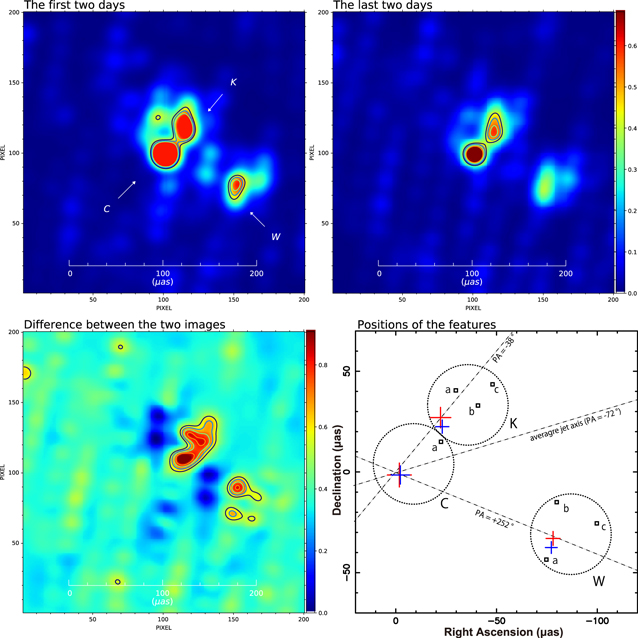
Figure 7. Images of the central core region: the top left panel is the image obtained from the data of the first two days. The upper right panel is that obtained from the data of the last two days. In both images, the CLEAN components are grouped and convolved with the restoring beam of a circular Gaussian with HPBW of 20 μas. The brightness distribution is shown in pseudo-color (arbitrary unit). As shown in the upper left panel, three features, C (core), K (knot), and W (west component), were detected. The lower left panel shows the difference between the last image and the first image, i.e., the time variation of the brightness distribution during 5 days. The lower right panel shows the positions of the C, K, and W peaks. The red crosses are for the first two days, and the blue crosses are for the last two days. The size of the crosses is ten times the size of the error bars in position. The small squares also indicate the location of the large increase in intensity.
Download figure:
Standard image High-resolution imageThe high spatial resolution of the EHT array clearly shows the presence of two bright peaks, i.e., the core and knot structure. The core is indicated by “C” and the knot by “K” in the upper left panel of Figure 7. In addition, we found a feature, “W”, located west about 83 μas apart from the core C. The flux densities from the obtained CLEAN components are FC ∼ 60 mJy for the core (C), FK ∼ 40 mJy for the knot (K), and FW ∼ 25 mJy for the west feature (W). In this observation, the solid angle of features was not so clear. Here, we assume that the solid angle of the emission is 15 μas in diameter, and calculate the brightness temperatures (lower limit). The average brightness of feature C is Tb = 1.1 × 10¹⁰ K. Feature K has a brightness of Tb = 7.1 × 10⁹ K. Feature W is Tb = 4.7 × 10⁹ K. Thus, we have detected the central features with brightness temperatures higher than the EHTC ring (up to Tb ∼ 6 × 10⁹ K). The solid angle assumed here is the maximum size of a single, smoothed object that the EHT array can detect in the 230 GHz (Appendix A). Therefore, the actual brightness temperature is likely to be much higher. If the solid angle of the emission is 5 μas in diameter, the brightness temperature of core C reaches 1011 K. If this is the case, the brightness temperature is an order of magnitude higher than the previous measurement cases (Akiyama et al. 2015; Hada et al. 2016; Kim et al. 2018). This is mainly because the size of the emitting region has been identified as smaller due to the higher spatial resolution.
High brightness temperatures were often detected from some AGNs (Horiuchi et al. 2004; Homan et al. 2006), and can be explained by the Doppler boosting effect of relativistic motion of jet approaching toward us. Previous observations found no high-velocity movement in the M87 central core. Therefore, the brightness temperatures are not due to such Doppler boosting effects. If they actually reflect the physical temperatures, they can be explained easily by the simple radiatively inefficient accretion flow (RIAF) disks (Kato et al. 2008; Nakamura et al. 1997). Our observational results are consistent with those of previous studies, supporting the existence of the RIAF disk in the M87 core (Di Matteo et al. 2003).
There is a clear difference between the two images observed over the five days. According to The Event Horizon Telescope Collaboration et al. (2019c), they found a change in the closure phase between data sets from the first two days and the last two days. In other words, there was a clear time variation. However, the EHTC could not clearly identify from the structure of that ring where that change occurred (The Event Horizon Telescope Collaboration et al. 2019d). We identified the change in the closure phase as due to a change in the core-knot structure (features C and K). In particular, the change in the position of feature K was also seen in the trial images during the hybrid mapping process.
Assuming that the features are single components, we fitted a Gaussian brightness distribution to each feature and measured the central position and displacement over five days. Relative to the position of feature C, the change in position of feature K is Δα = −0.4 μas, Δδ = −4.5 μas in 5 days, and the proper motion is 0.33 mas yr−1 (v ∼ 0.1c). Feature K appears to be approaching feature C as if showing an inflow motion. However, if we look at the differences in the brightness distributions shown in the lower left of Figure 7, we can see that the changes in the brightness distribution of feature K occur in three places, all at the north end of feature K. In the latter measurement of the position of feature K, feature K appears to be moving south because the brightness distribution of feature C affects the measurement; K is moving north on the line of PA = −38° as a whole. The position of feature C has hardly changed, except for the location of “a” where the intensity increased is at the northwest side of feature C. In other words, the structure of features C and K and their time variation can be interpreted as an outflow emanating in the direction of PA = −38° from the origin. There has never been a measurement of the motion of a knot so close to the central core.
In comparison, it is difficult to interpret what feature W is. Three hypotheses are presented below.
- 1.Gravitational lensing image. Feature W is morphologically similar to feature K, and the pattern of brightness variation is also similar. This can be attributed to the formation of the gravitational lens image of feature K due to the strong gravitational field of the SMBH in M87. Assuming that the position of SMBH is approximately equal to the position of feature C (the distance between the core of M87 and SMBH is 41 μas or 6 RS; Hada et al. 2011), feature W would be located (or at least projected) at 12 RS from the SMBH. There is a possibility that the radio waves emitting from feature K to the far side, orbiting in the strong gravity field of the SMBH, and being changed the propagation direction, come toward us (black hole echo; Saida 2017; Virbhadra 2009; Virbhadra & Ellis 2000). If feature W is such a lensing image caused by the strong gravity field of the SMBH, it should be the image of the backside of feature K, so it is most likely a mirror image of feature K. However, the shape of feature W does not look like such an image. Needless to say, there are many possibilities for a gravitational lensing due to a strong gravity field, so detailed calculations are required to deny it completely; however, the possibility that feature W is a gravitational lensing image is not very high.
- 2.Another central black hole. Feature C is the primary SMBH of M87, and feature W is a secondary SMBH orbiting the primary SMBH. If there is a binary SMBH in M87, it can be permanently observed with the EHT array. Based on these observations, we calculated two possible orbits.
- (a)The proper motion of feature W (μ = 0.34 mas/yr, v ∼ 0.09 c ) is assumed to be due to a circular orbit motion, and its orbital radius is assumed to be the separation R = 83 μas from feature C. In this case, the orbital period T is ∼1.5 yr, If the real radius is R = 1.4 × 10³ au, the mass of central object Mc is only 1.2 × 10⁶ M⊙. Since the estimated mass is too small as compared to those of the previous M87 studies, this assumption must be rejected.
- (b)We assume that the observed proper motions and structure change of feature W are only due to the changes in surrounding matters, and that the measured proper motions of feature W have nothing to do with its orbital motion. In other words, we assume here that no change in the position of the center of gravity of feature W is observed. Also, it is assumed that feature C has a SMBH with a mass of 6 × 10⁹ M⊙ and that the orbital radius of feature W is the distance between features C and W. The distance between them is 83 μas (1.4 × 10³ au or 11.9 RS). It is consistent with the 86 GHz core size of ∼80 μas at 86 GHz observed in 2014 (Hada et al. 2016), suggesting that the two features C and W are not transient. Also the sinusoidal oscillations of the position angle of the jet were observed with a period of roughly 8 to 10 yr (Walker et al. 2018). If the two features, C and W, compose a binary of black holes, its orbital motion can cause such jet oscillations. Certainly, the apparent separation of approximately 1.4 × 10³ au is too short to explain the observed period of the jet oscillation. However, if the real distance is longer by a factor of about 3.42, which is the correction factor of the viewing angle of the jet axis from us (∼17°), the orbital period of the binary can be ∼10 yr.
- 3.Unstable initial knot. Feature W is another knot moving toward a different direction. The jet of M87 is known to have a wide opening angle at scales well below 1 mas (Junor et al. 1999). Furthermore, Walker et al. (2018) found evidence from 43 GHz observations that the initial opening angle θapp is ∼70°. We found the angle ∠KCW is 70°, and further that the line of the average jet axis (PA = −72°) divides this angle almost evenly into 34°, and 36°. Furthermore, the lines CK and CW extend in the directions of PA = −38° and PA = 252°, respectively. These directions are very similar to those of the ridges observed at 43 GHz from where Walker et al. (2018) measured the initial opening angle. We guess that not only feature K but also feature W are initial knots that have just emerged from the core; and still, the shape is very unstable and shows large and rapid changes.
Adopting the most conservative hypothesis, feature W, like feature K, can be understood to be a knot that represents the initial jet structure.
As we will discuss in Section 4.3.2, the core-knot structure (features C and K) is robust in the sense that it can be obtained with different imaging parameters. On the other hand, the 40 μas ring of the EHTC is sensitive to BOX parameters and can be easily destroyed, even if it can be created as shown in Section 5.7. Due to the robustness of the core-knot structure, we consider it to be a real structure. On the other hand, the feature W is sensitive to the BOX size, so its detection is not as reliable as it could be. However, the structure corresponding to feature W had already appeared in the first imaging results (Section 3.2.2). That is, feature c in Table 3 is in a similar position to feature W and also shows the largest asymmetry. Also, if we run the EHTC-DIFMAP pipeline without its BOX setting, an emission feature appears at the position close to feature W (lower right panel of Figure 24). These suggest that the feature W is also a real structure.
4.2. The Jet
Here, we show the overall brightness distribution (Section 4.2.1) and that of the so-called jet launching region, which is a few milliarcseconds away from the core (Section 4.2.2).
4.2.1. The Overall Structure
Figure 8 shows the overall structure of the M87 we obtained. In order to make the emission obvious, we used a restoring beam of 200 μas circular Gaussian, 10 times larger than the default beam size. As already mentioned, it is found that the emission at 230 GHz comes not only from the central point source but also from other regions.
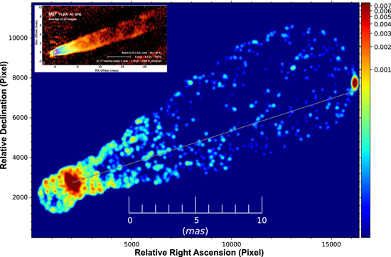
Figure 8. The overall structure of M87 we obtained (image from the data of the last two days). The gray line shows the average direction of the jet axis (PA = −72° from Walker et al. 2018). The restoring beam is 200 μas circular Gaussian, which is much larger than the default beam in order to make the emission obvious. The logarithmic pseudo-color (arbitrary unit) is used to enhance the darker parts of the image. The image consists only of the grouped-CLEAN components obtained. For comparison, the average image at 43 GHz from VLBA observations taken from Figure 1 in Walker et al. (2018) is shown in the inset. The bright spot seen on the right (west) edge is not the real brightness distribution (see Section 3.4).
Download figure:
Standard image High-resolution imageThe EHTC apparently assumed or concluded that there is no bright source outside the narrow region (128 μas in diameter) where the ring was found. However, we found that the emission was not from such a narrow range, but from a wide range of more than a few milliarcseconds. This is consistent with the results of VLBI observations at 43 GHz and 86 GHz.
Our final image shows a similar structure to the average image in the 43 GHz band (the inset of Figure 8). There are two main similarities.
First, as in the 43 GHz image, our image shows that the jet has an extended structure leading to the core. Then, up to a few milliarcseconds away from the core along the jet axis, both edges are bright, as in the previous observations.
Second, the brightness distribution of the jet in the 230 GHz is consistent with the trend of those obtained from lower-frequency observations. The core is vastly brighter than the jet structure. Within the radius of 0.25 mas (250 μas) from the center, 63% (the first two days’ image) and 75% (the last two days’ image) of all obtained flux densities are concentrated. However, features C, K, and W (several tens millijanskys at most, see Table 5) do not occupy them, rather the flux densities are distributed over a wider area. In contrast, the EHTC rings have a total of about 500 mJy that is contained entirely within a diameter of only a few tens of microarcseconds.
Table 5. Properties of Main Features: Positional Offsets from the Map Phase Center in μas, Flux Densities in mJy, and Minimum Brightness Temperatures in Kelvin Calculated with the Assumption That the Emission Area Is 15 μas in Diameter
| The First Two Days’ | The Last Two Days’ | |||
|---|---|---|---|---|
| Peak Position | R.A. (μas) | δ (μas) | R.A. (μas) | δ (μas) |
| Core | −1.8 ± 0.6 | −1.5 ± 0.6 | −2.3 ± 0.5 | −1.5 ± 0.5 |
| Knot | −22.2 ± 0.5 | 27.0 ± 0.5 | −23.1 ± 0.3 | 22.5 ± 0.3 |
| West | −78.1 ± 0.3 | −33.0 ± 0.3 | −77.2 ± 0.3 | −37.5 ± 0.3 |
| Δ R.A. (μas) | Δδ (μas) | |||
| Core | −0.5 | 0.0 | ||
| Knot | −0.9 | −4.5 | ||
| West | 0.9 | −4.5 | ||
| Position of intensity increase | R.A. (μas) | δ (μas) | ||
| Core area a | −22.4 ± 0.4 | 15.0 ± 0.4 | ||
| Knot area a | −29.8 ± 0.7 | 40.5 ± 0.7 | ||
| b | −40.8 ± 0.3 | 33.0 ± 0.3 | ||
| c | −48.0 ± 0.4 | 43.5 ± 0.4 | ||
| West area a | −74.7 ± 0.7 | −43.5 ± 0.7 | ||
| b | −79.9 ± 0.5 | −15.0 ± 0.5 | ||
| c | −99.8 ± 0.7 | −25.5 ± 0.7 | ||
| Integrated intensity | (mJy) | (mJy) | ||
| Core | 55.6 ± 5.2 | 66.1 ± 4.7 | ||
| Knot | 33.5 ± 2.7 | 44.9 ± 2.3 | ||
| West | 22.5 ± 1.2 | 30.2 ± 1.4 | ||
| Brightness temperature | (K) | (K) | ||
| Core | >1.0 × 10¹⁰ | >1.2 × 10¹⁰ | ||
| Knot | >6.0 × 10 9 | >8.1 × 10 9 | ||
| West | >4.0 × 10 9 | >5.4 × 10 9 | ||
| Grouped-CLEAN components | (mJy) | (mJy) | ||
| FGCC > 0.1 mJy | 707.4 (n = 1151) | 1032.6 (n = 1657) | ||
| All | 767.8 (n = 2824) | 1154.6 (n = 7844) | ||
Note. Positions of intensity increase in features are also shown. At the bottom, the sum-up intensities and the numbers of the grouped-CLEAN components in the whole images are shown.
Download table as: ASCIITypeset image
The results of this observation at 230 GHz show that the brightness in the jet region is orders of magnitude lower than that in the core region. In addition, the decay of the flux density along the jet is more rapid at 230 GHz than in the lower-frequency observations. Compared to the peak luminosity of the core, the relative intensities are 6.6 × 10⁻² at 0.25 mas from the core, 9.9 × 10⁻³ at 0.5 mas, and 2.3 × 10⁻³ at 1 mas (Figure 9). While, in the observation at 43 GHz, the decreases of intensity are 2.8 × 10⁻¹ at 0.25 mas from the core peak, 8.5 × 10⁻² at 0.5 mas, and 2.5 × 10⁻² at 1 mas (from the upper panel of Figure 6 in Walker et al. 2018). At 1 mas position, the intensity of the jet structure is 2.5% of the core peak at 43 GHz; however the intensity at 230 GHz is only 0.2% of the core peak, namely the intensity of the jet structure is greatly attenuated at 230 GHz. However, with respect to the structure of the brightness and intensity distribution of both edges, the trend is in good agreement with the previous results of the M87 jet.
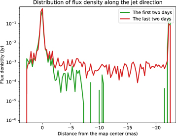
Figure 9. Flux density distribution corrected for the bandwidth smearing effects. Here we show the sum of the flux densities of the CLEAN components obtained in each small region. The horizontal axis shows the distance along the average direction of the jet axis (PA = −72° from Walker et al. 2018) from the map center (near the peak of the core). The binning intervals are 0.25 mas. The vertical axis shows the sum of the flux densities in Jy (logarithmic scale). The green line shows the flux density distribution for the image from data of the first two days, and the red line shows the flux density distribution for the image from data of the last two days. The peaks seen on the right edge are not real flux densities (see Section 3.4).
Download figure:
Standard image High-resolution imageThe total flux density measured by the EHTC (The Event Horizon Telescope Collaboration et al. 2019c) was 1.12 and 1.18 Jy, for the first two days and the last two days, respectively. In contrast, the total flux density of the CLEAN component in our analysis is 767.8 and 1154.6 mJy, respectively. That is, there are missing flux densities of 353 and 25.4 mJy, respectively. 12
The difference between the total flux density of our image and the single-dish flux density is most likely due to the presence of extended emission somewhere, which the present EHT array cannot detect. As shown in Appendix A, the EHT array cannot detect a smoothed emission feature (like Gaussian brightness distributions) with size larger than 30 μas.
4.2.2. The Jet Launching Region
In this section, we present the structure within a few milliarcseconds from the core. We have found emission belonging to the jet component that was not detected by the EHTC.
In Figure 10, the brightness distribution in this region is represented in three ways. The logarithmic pseudo-color (arbitrary unit) is used to represent the large differences in brightness distribution. The upper panels (a) and (b) are composed by restoring beams of a circular Gaussian with half-power beam width (HPBW) of 20 μas, which corresponds to the size of the spatial resolution of the EHT array for M87 observations. The middle panels (c) and (d) are composed by restoring beams of circular Gaussian with HPBW of 200 μas. In order to facilitate a comparison with previous results, the beam size is close to the spatial resolution of previous lower-frequency observations (43, 86 GHz). Panels (e) and (f) in the bottom row show the image by the large restoring beam overlaid with the 43 GHz averaged image by the VLBA (Walker et al. 2018). Note that the 43 GHz image is time-averaged over 17 yr, so the knot-like features have been averaged out. It can be seen that the brightness distribution at 230 GHz is consistent with that at 43 GHz. The left panels (a), (c), and (e) show images of the data from the first two days. Panels (b), (d), and (f) on the right show images of the data from the last two days. Obviously, they are different from each other. However, the differences seen in the regions of a few milliarcseconds cannot be attributed to the intrinsic variability of the source that occurred during the five days. Rather, it seems to be mainly dependent on the observational conditions.
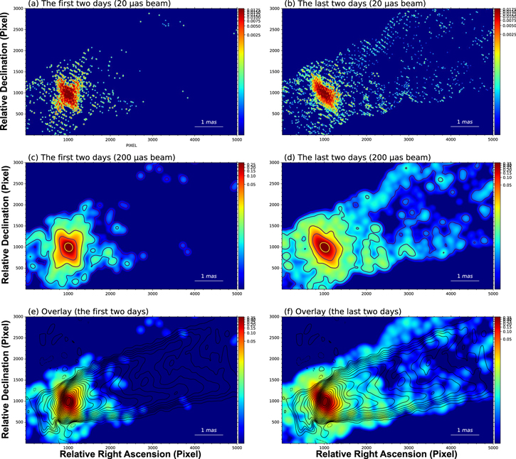
Figure 10. Images of the core and the jet launching region: panels (a), (c), and (e) on the left show images of data from the first two days. The right panels (b), (d), and (f) show the images of data from the last two days. The logarithmic pseudo-color (arbitrary unit) is used to represent the large differences in brightness distribution. The upper panels (a) and (b) are composed by a circular Gaussian restoring beam with HPBW of 20 μas. The middle panels (c) and (d) are composed by a circular Gaussian restoring beam with HPBW of 200 μas. The levels of contour lines in the panels (c) and (d) are 10−5, 10−4, 10−3, 10−2, and 10−1 of the peak brightness. The lower two panels, (e) and (f), show overlaid ones with the VLBA averaged image at 43 GHz. The contour lines show the VLBA averaged image at 43 GHz taken from Figure 3 in Walker et al. (2018), and the levels of contour lines are −0.3, 0.3, 0.6, 0.85, 1.2, 1.7 mJy beam−1. Their restoring beam shape is 0.43 × 0.21 mas with PA = −16°. Peak positions of the two images are used for the alignment of the two images.
Download figure:
Standard image High-resolution imageThe emission areas of our 230 GHz results are consistent with that of the 43 GHz average image. They also show that both edges of the jet are brightened, which have been observed in 43 and 86 GHz. Based on our data analysis, it seems that the detection of emissions in the range of several milliarcseconds from the core of the M87 has been successful to some extent.
4.3. Reliability of Our Final Images
As mentioned in Section 3, our calibration method was limited to self-calibration because the public the EHTC data do not contain raw data.
We also had to give up on the amplitude self-calibration because the closure phase residuals were not reduced as compared to the case when only phase calibration was performed. Therefore, the calibration is not yet fully complete. As clues to the reliability, we describe the properties of the final images from three aspects: detection limit (Section 4.3.1), robustness (Section 4.3.2), and the self-consistency of our imaging (Section 4.3.3), where our images show better self-consistency than those of the EHTC.
4.3.1. From Sensitivity
The Event Horizon Telescope Collaboration et al. (2019c) shows that the typical sensitivity of a baseline connected to ALMA is ∼ 1 mJy. We estimate that this sensitivity is for an integration of about 5 minutes. For an on-source time of 2 days, the attainable sensitivity reaches close to 0.1 mJy (ALMA-LMT baseline, S/N = 4, assuming a point source). It is difficult to estimate the practical sensitivity of the synthesized image of an interferometer composed of antennas with different performances, such as the EHT array. However, it is unlikely that the image sensitivity will not be worse than the baseline sensitivity noted above.
Here, we consider 0.1 mJy to be a reliable detection limit for our final images. Figure 11 shows the distribution of the grouped-CLEAN components with flux densities larger than 0.1 mJy. Almost all of the components are concentrated within a few milliarcseconds of the core. (The remaining components are located in a false bright spot created outside the range of this figure, about 20 mas west of the center.) The image from the core to a few milliarcseconds along the average jet axis seems to be reliable in terms of detection limits.
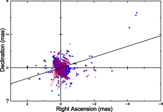
Figure 11. Distributions of the grouped-CLEAN components with flux densities larger than 0.1 mJy. Red dots are from the image of the first two days, blue dots are from the image of the last two days. The sloped line indicates the average direction of the jet axis (PA = −72° from Walker et al. (2018)).
Download figure:
Standard image High-resolution imageA large number of grouped-CLEAN components with flux densities larger than 0.1 mJy are found in our final images. The number of grouped-CLEAN components with flux densities larger than 0.1 mJy is 1151 from the images of the first two days (with a sum of flux density of 707.4 mJy), and 1657 from the images of the last two days (with a sum of flux density of 1032.6 mJy; Table 5).
4.3.2. The Robustness of Our Final Image
In this section, we discuss another property of our final images: the robustness of the image structure.
If the data is not yet completely calibrated, BOX technique is effective. As well as the EHTC, we also used the BOX technique to limit the imaging area (FOV). This technique has the potential to produce good images even if the calibration is incomplete. On the other hand, it may create structures that do not actually exist. In fact, the bright spot on the right-hand side of our final image (Figure 8) is such an example. Therefore, care must be taken when using the BOX technique, because a false structure will be created in the BOX area, and the real structure outside of the BOX area will be removed from the image.
We examine how the image is affected when we change the BOX parameters. In other words, we investigate the stability of the image. We compare the images obtained by changing the size of the BOX. The panels in Figure 12 show the four cases. The upper left panel (a) is the image without BOX (the FOV is 24.576 mas square). The top right panel (b) shows the image with the same 8 BOXes that we used to obtain our final images. The lower right panel (c) is the image with a small BOX (circle with diameter D = 5 mas is used). The lower right panel (d) is the image with a very narrow BOX (circle with diameter D = 128 μas that corresponds to the FOV the EHTC used). These four CLEAN images were produced using data of the entire four days.
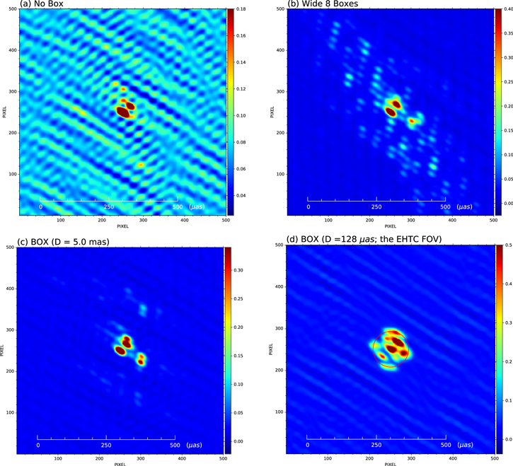
Figure 12. Comparison of images obtained by changing the size of Box. Panel (a) is the image without BOX (the FOV is 24.576 mas square). Panel (b) shows the image with the same 8 BOXes that we used to obtain our final images. Panel (c) is the image with a small BOX (circle with diameter D = 5 mas is used). Panel (d) is the image with a very narrow BOX (circle with diameter D = 128 μas that corresponds to the FOV the EHTC used). These four CLEAN images were produced using data of the entire four days.
Download figure:
Standard image High-resolution imageIn all panels, the emission can be seen at the positions of features C (core) and K (knots). On the other hand, feature W disappears in the case where the BOX setting is omitted (no BOX case). In the case of the EHTC FOV, no emission is seen at the position of feature W because the position of feature W is outside the BOX setting.
Without the BOX setting, the S/N of the image is degraded. From the comparison between panel (a) and the other panels, we can see that the BOX setting compensates for the lack of calibration and improves the image quality. Thus, the presence or absence of the BOX setting seems to have an effect on the image quality. Another noteworthy point is that, in the case of the very narrow BOX setting (panel (d)), several different bright spots newly appear in the BOX. Moreover, some of them are located at the boundaries of the BOX. In such a case, other actual brightness distributions could exist outside the BOX setting.
Since feature W disappears in the CLEAN image without the BOX setting, feature W is considered to be less reliable than features C and K. As mentioned at the end of Section 4.1, there are other reasons to consider that feature W has a real existence.
4.3.3. Self-consistency of Our Imaging as Compared to Those of the EHTC Images
At the end of this section on image reliability, we present the degree of matching between the visibility and the image model. Here, we compare the results with those of the EHTC ring.
- 1.Relations between the visibility amplitude and u−v distance (projected baseline length). The amplitude of visibility obtained by the inverse Fourier transform of the image model is compared with those of the observed visibility data. Figures 13, and 14 correspond to Figure 12 in The Event Horizon Telescope Collaboration et al. (2019d). This kind of comparison of visibilities is often performed to check the reliability of an image. However, here, the observed visibility data are calibrated by self-calibration solutions using the image model. Therefore, it is important to note that the amplitudes of the observed visibility data and those from the image model are no longer independent of each other. What can be safely determined from this comparison is the internal consistency of the imaging and calibration process. Figure 13 shows the data from the first two days, and Figure 14 shows the data from the last two days. The top row of each figure shows the variation of the visibility amplitude with respect to the projected baseline length. The red dots are those of the image model. The middle and bottom panels show the normalized residual amplitudes between the image model and the calibrated observation data. The plotted points are the calibrated raw data that have not been time-integrated, and we can see that the scatter is much larger than that in their Figure 12 (The Event Horizon Telescope Collaboration et al. 2019d), where the time-integrated points have been plotted. We can see that the average and standard deviation of the normalized residuals of our final image are much smaller than that of any of the EHTC ring images in Figure 15. As an example, we show the normalized residual values for t = 180 s integration.For the data of the first two days, our image shows NRours = 0.030 ± 0.539, while the EHTC images show NREHTC = 0.148 ± 0.933.For the data of the last two days, our image shows NRours = 0.127 ± 1.259, while the EHTC images show NREHTC = 0.589 ± 2.370. Here, in the case of EHTC, we used the simple averages of those values for the four EHTC images. One thing that interests us is the large discrepancy in amplitude of the EHTC ring image cases at the longest baseline lengths over 8 × 10⁹ λ. It is three times larger than those of our final image cases. Since the EHTC ring images are very compact, if the images are really correct, the amplitude residuals at the longer baseline should become small at least. Another thing that interests us is the amplitudes at the very shorter baselines that are nearly zero λ. They contain the components of the extended structure that are resolved by high spatial resolution by EHT, so it is not surprising if they do not match. Our images reproduce the amplitudes of the very short baselines well. The differences are more significant in the cases of the EHTC rings. In our cases, the normalized residuals are 4 at most, but in the cases of the EHTC rings, they are distributed widely in the range of 0–15, which is not surprising since the EHTC rings are compact and have no extended components. However, in Figure 12 in The Event Horizon Telescope Collaboration et al. (2019d), the maximum is 4, as if the result shows good self-consistency. The EHTC Figure also shows the same results for the normalized residuals at the longest baselines. This is not consistent with our own analysis. Perhaps a different integration time of the data may cause this apparent discrepancy. (There is no explanation for the integration time of the data points in Figure 12 in The Event Horizon Telescope Collaboration et al. (2019d). Since the scatter of data points is affected by thermal noise, its value changes depending on the integration time of the data. Therefore, we examined the amounts of normalized residuals by changing the integration time. Figure 15 shows the average and standard deviation of the obtained normalized residuals. It can be seen that, at any integration time, our final image always shows smaller values than that of the EHTC ring image. The averages of the 10 s integrations and integrations over 180 s differ by a factor of 3, which explains the discrepancy above.The diagram of the visibility amplitude and u−v distance shows that our final images, both the first and the last days, show a better consistency of imaging and calibration processing compared to the cases of the EHTC ring images. The diagrams indicate that our images, not those of EHTC, are supported by the data.
- 2.Closure phase variations. Following Figure 13 of The Event Horizon Telescope Collaboration et al. (2019d), we show the closure phases of the observed data and those derived from image models for some triangles in Figure 16. We added the closure phases of ALMA-LMT-SMA and LMT-PV-SMA to the three triangles (ALMA-LMT-PV, ALMA-SMT-LMT, SMT-LMT-SMA) shown by the EHTC. Closure phase is a quantity that is free from systematic phase errors and reflects the observed source structure. All panels in Figure 16 show large phase variations, which correspond not to time variation in the structure of the observed source, but to time variation of the shape of the triangle composed by the three stations as seen from the observed source. The green dots are the closure phase corresponding to the EHTC ring image, and the red dots correspond to our image. The dots of our image (green dots) appear to be better aligned with the observed data than those of the EHTC ring image. Our image is more complex than the EHTC ring, resulting in short-term small closure phase variations.The three panels from the top right toward the bottom correspond to the panels shown in Figure 13 of The Event Horizon Telescope Collaboration et al. (2019d). In the case of the two triangles ALMA-LMT-PV and SMT-LMT-SMA, our results are consistent with those of EHTC. However, our results for the closure phase in ALMA-SMT-LMT triangle differ from those of EHTC. In our case, the closure phase shows an increase from +25° to +85°, while that of the EHTC shows a decrease from −25° to −80°. Both the first and last values and the amount of change are opposite in positive and negative. All triangles were examined, but none were identical to the closure phase variation shown by the EHTC for the ALMA-SMT-LMT triangle. Our closure phase values are from the AIPS task, CLPLT. All triangles were examined, and none showed the variation similar to that the EHTC showed for the triangle. Also, there are no significant closure phase discrepancies between the real and model data. There seems nothing wrong with the CLPLT calculations. In our analysis, there is no clear difference in closure phase matching between our images and the EHTC rings. A notable difference is in the case of the LMT-PV-SMA triangle, where the closure phase in the EHTC rings is beyond ±3σ error bars, whereas in our final images, it manages to fall within it.The values of the closure phases also change depending on the integration time of the data; however, even when the integration time is changed, the residuals of either of them do not become overwhelmingly small. Figure 17 shows the statistics of the closure phase residuals for all triangles. As far as the closure phase residuals are concerned, between our images and the EHTC rings, there is no significant difference. Our image of the core-knot structure shows the same magnitude of closure phase residuals as those of the EHTC ring image. As an example, we show the standard deviations of the closure phase residuals at t = 180 s integration. For the data of the first two days, our image shows σours = 40°.5, while the EHTC image shows σEHTC = 38°.5. For the data of the last two days, our image shows σours = 43°.2, while the EHTC image shows σEHTC = 43°.7. As for closure phase residual, there is no significant difference between ours and the EHTC rings. If we claim that the EHTC ring image is correct due to the closure phase residual, then our images are also correct. 13 If these residuals are due to thermal noise, they should decrease inversely proportional to the root square of the integration time T, but as Figure 16 shows, they do not decrease in that way. It means that both images of ours and those of the EHTC still have differences from the true image.
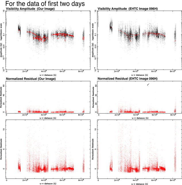
Figure 13. Relation between the visibility amplitude and u−v distance for the first two days of data. The left panels are for our image, and the right panels are for the EHTC ring image model with the EHTC DIFMAP pipeline using 096H data (April 6). Every dot is a raw visibility point for a 10 s integration. The top panels show the plots of visibility amplitude vs. u−v distance. The black dots in them show those calibrated by self-calibration solutions using the image model. The red dots are those from the Fourier-transformation of the image model. The middle and bottom panels show normalized amplitude residuals. The middle panel shows all data points. The vertical axis scale is very large due to data points with very large values, as indicated by black lines. The bottom panels show a magnified view of the range of normalized residuals from −5 to +15. In all cases, the minimum value of the normalized residuals is greater than −1.
Download figure:
Standard image High-resolution image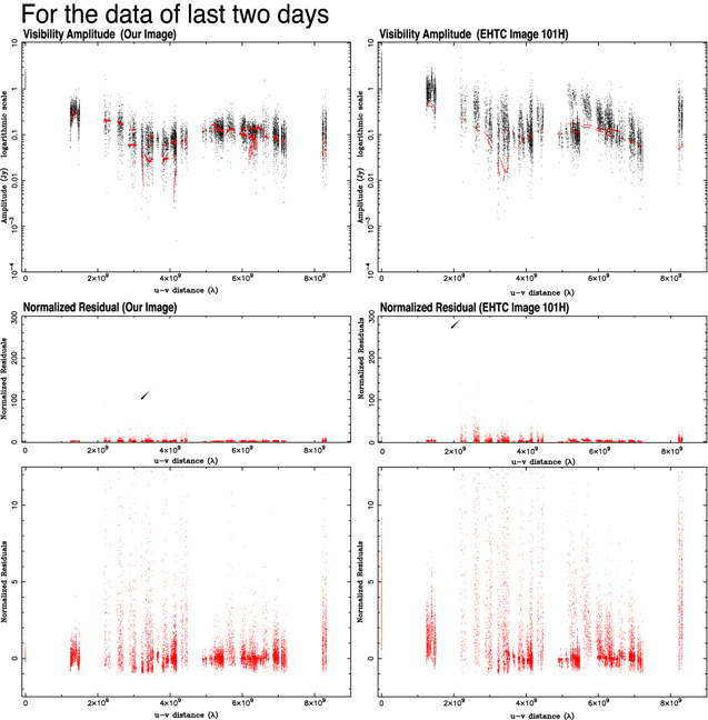
Figure 14. Relation between the visibility amplitude and u−v distance for the last two days of data. The left panels are for our image, and the right panels are for the EHTC ring image model with the EHTC DIFMAP pipeline using 101H data (April 11). Every dot is a raw visibility point for a 10 s integration. The top panels show the plots of visibility amplitude vs. u−v distance. The black dots in them show those calibrated by self-calibration solutions using the image model. The red dots are those from the Fourier-transformation of the image model. The middle and bottom panels show normalized amplitude residuals. The middle panel shows all data points. The vertical axis scale is very large due to data points with very large values, as indicated by black lines. The bottom panels show a magnified view of the range of normalized residuals from −5 to +15. In all cases, the minimum value of the normalized residuals is greater than −1.
Download figure:
Standard image High-resolution image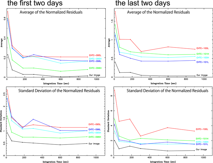
Figure 15. Statistics of normalized residuals. The upper panels show the average values of the normalized residuals. The lower panels show the standard deviations. The left panels are the data of the first two days, and the right ones are the data of the last two days. The black line shows the case of our final image, and other color lines show the cases of the EHTC images.
Download figure:
Standard image High-resolution image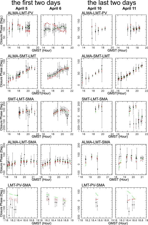
Figure 16. Closure phase variations of five triangles (ALMA-LMT-PV, ALMA-SMT-LMT, SMT-LMT-SMA, ALMA-LMT-SMA, and LMT-PV-SMA). Closure phases of the observed data are shown by black dots with ±3σ error bars, which are obtained from 5 minutes integration. Red dots show those from our image models. Green dots show those from EHTC ring image models (the EHTC 096H image for the first two days’ data, the EHTC 101H image for the last two days).
Download figure:
Standard image High-resolution image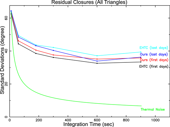
Figure 17. Standard deviations of the closure phase residuals from all triangles. The case of the EHTC image (for the first two days) is shown as a black line, and for the last two days as a cyan line. The cases of our final images are shown as a red line for the first days and blue line for the last days. The green line shows the case that the residuals are due from thermal noise.
Download figure:
Standard image High-resolution image5. Why the EHTC Found Their ∼40 μas Ring?
In Sections 3 and 4, we tried to reconstruct the image from the EHT public data using the hybrid mapping process. Our final images contain a core-knot structure at the center and features along the jet axis toward the outside. It is consistent with those obtained by 43 GHz or 86 GHz observations. On the other hand, three of the EHTC imaging analyses all obtained ∼40 μas rings similar to each other, but no jet structure. In this section, we show the evidences that the EHTC ring is an artifact.
The essential reason why the ring image was obtained by all the EHTC imaging analyses is the limited u−v coverage of the EHT array for M87, namely the data sampling bias; though the EHTC realized 230 GHz VLBI observations on a scale that has never been accomplished before. In addition, the very narrow FOV settings of the EHTC strongly help to create ∼40 μas ring shape from the EHT u−v data sampling bias.
First, in Section 5.1, we discuss the nature of the u−v coverage of EHT for the M87 observations. The spatial Fourier components for the fringe spacing of ∼40 μas are lacking. Second, in Section 5.2, we discuss how the dirty beam (PSF) of the M87 EHT observations is affected by this lack of the spatial Fourier components for the fringe spacing of ∼40 μas. Third, in Section 5.3, we show that the dirty map is greatly affected by the PSF shape in the case of the EHTC data. Fourth, in Section 5.4, we show that even from the simulated visibility data of a point source we can create ∼40 μas rings. This means that the u−v coverage of the EHT array for M87 can create the ∼40 μas ring regardless of the real structure of the observed object. In other words, the EHTC result is indistinguishable from an artifact. Fifth, in Section 5.5, we investigate one of their open procedures for imaging demonstration. The EHTC used three methods for their imaging. We investigated their DIFMAP (Shepherd 1997) pipeline, which is the closest to traditional procedures for VLBI, and found an improper point. In the EHTC-DIFMAP pipeline, they adopted a very narrow FOV setting by using the BOX technique. When we ran the EHTC-DIFMAP pipeline without the BOX, the 40 μas ring disappeared. Instead, a core-knot structure appeared. We also checked the output of the simulated data for other shape model images and found that the EHTC-DIFMAP pipeline did not reproduce the input model images correctly. In other words, the EHTC-DIFMAP pipeline does not prove the correctness of the EHTC ring image from the data. In addition, we estimate the amount of calibrations that the EHTC performed during their imaging process (by the DIFMAP method), and compare them with those we did in our analysis. We found that a large amount of additional “calibrations” are required to make the 40 μas ring (Section 5.6). Also, we discuss the robustness of the EHTC ∼40 μas ring structure in Section 5.7. The structure is sensitive to the imaging parameters. If we increase the BOX size, the ring image changes significantly.
Despite their “isolated image analysis” and surveys involving large-scale simulations, the EHTC have obtained artificial ring images. Finally, we explain in Section 5.8 why their objective survey has produced artifacts. They determined their optimal imaging parameters through large-scale simulations. However, they did not take into account the sampling bias that tends to produce the ∼40 μas structure. The EHTC focused only on the reproducibility of the input image models and not on the simultaneous reproducibility of the input error models. It cannot be ruled out that their optimal parameters may have had the property of creating the EHTC’s ∼40 μas ring not by performing proper calibration and imaging, but rather by enhancing the sampling bias effect. The facts shown in this section are strong evidences that the EHTC ∼ 40 μas ring image is an artifact. In Section 5.9, we summarize the reasons why the EHTC obtained the artifact image unintentionally.
5.1. u−v Coverage of the EHT Array for M87
We here investigate the u−v sampling of the EHT array for M87 observations. The u−v coverage itself is shown in the EHTC Paper I (The Event Horizon Telescope Collaboration et al. 2019a). It shows a good u−v coverage as an interferometer of practically 5 stations and 10 baselines. We looked at the number of data samples from another point of view. Figure 18 shows the distribution of spatial Fourier components (fringe spacings) sampled by EHT for M87 during the four observational days. The number of sampled data is plotted against the fringe spacings in μas unit. We can see that there are no samples for ranges d = 26–28 μas, d = 44 −46 μas, and d = 95–100 μas. 14 The number of sampled data for the size of the EHT ring (d = 42 ± 3 μas) is quite small, and for spacing between d = 44–46 μas, there are no sampled data.
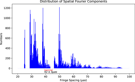
Figure 18. Distribution of the sampling data (all data of the four days from all baselines). The x-axis shows the fringe spacings of sampled visibility data in μas unit. The y-axis shows the number of sampled data. Here, samples larger than the fringe spacing of 100 μas are omitted. The red line segment indicates the range of the diameter of the ring measured by the EHTC (d = 42 ± 3 μas).
Download figure:
Standard image High-resolution imageThe few numbers of sampling around 42 μas fringe spacings should affect the imaging performance. In the following subsections, we investigate how this lack of spatial Fourier components can affect the imaging result.
5.2. Substructures in the Dirty Beam
The EHTC show no description of the dirty beam structure. We examine the dirty beam calculated from the u−v coverage. Dirty beam is the term used in the field of radio interferometry, and its meaning is the same as that of PSF in optics. In other words, it is the diffraction image of a single point when the data calibration is perfect. If we can obtain all spatial Fourier components, the dirty beam becomes a two-dimensional δ-function.
In practice, we can obtain only a limited sample of spatial Fourier components, and thus the dirty beam has a complex shape. Figure 19 shows the dirty beam of the EHT array on the first day observation of M87. The FWHM of the main beam is approximately 20 μas. We can see a point-symmetric pattern around the main beam. This pattern includes peaks lower than the main beam. Such peaks are often called sidelobes in radio astronomy. We can see that the distances between the main peak and the first peaks of sidelobes are about 45 μas. 15 The separation between them corresponds to the radial range for which the spatial Fourier components are missing, and is very close to the diameter of the EHTC ring (42 ± 3 μas). Thus, it is important to clarify whether or not this PSF structure has affected the ring image or not. In addition, in Appendix B we show other PSF shapes by different weightings of u−v points. Even in these PSF shapes, the separations between the main beam and adjacent sidelobes do not change much. They also show substructures with ∼40 μas spacings.
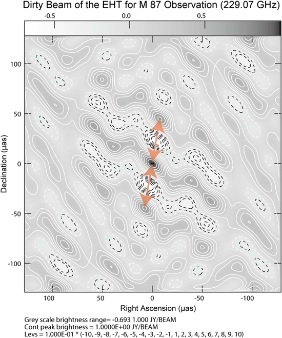
Figure 19. Point-spread function (dirty beam) of EHT on the first day of observation of M87. The contour levels are at every 10% points of the peak from −100% to 100%. Positive levels are shown by white lines, and negative levels by black dotted lines. The white dotted lines are for zero levels. The gray scale ranges from the minimum to the maximum brightness of the dirty beam image. The first sidelobe levels reach more than 70% of the height of the main beam. We put two red arrows with a length of 45 μas between the main beam and the first sidelobes. For the dirty beam image, we set the parameter ROBUST = 0 in IMAGR (its default setting).
Download figure:
Standard image High-resolution image5.3. The Relation between the Dirty Map Convolved by the PSF Shape and the Ring Structure
Here, we show what happens if we are not very careful in using the dirty map when applying the hybrid mapping process. A dirty map is an image created by simply performing an inverse Fourier transform on the obtained spatial Fourier components. Therefore, it is influenced by the data sampling bias, that is, the structure of PSF is convoluted into the dirty map. Furthermore, if the data calibration is insufficient, it will be reflected in the dirty map, and the obtained structure in such a dirty map can be far from the actual image. Therefore, it is dangerous to perform self-calibration using the dirty map as the image model.
It is clear that, in the case of multielement radio interferometers like ALMA, or VLA, the dirty beams have sharp main beams and very low sidelobes. Only in such cases, it is not so dangerous to estimate the true image by the dirty map. While, in the case of VLBI observations, the dirty beam is comparatively dirty, usually; we do not estimate the true image from them and do not use them as the model image for self-calibration.
We, however, try that here and show what happens. The left-side panels of Figure 20 show the dirty maps from the data of the first day of observations by EHT. To obtain these maps, we applied the phase-only calibration by the self-calibration technique using a point source as the image model. We can see a ring-like structure at the center, and many images that look like the ghosts of this central ring-like structure.
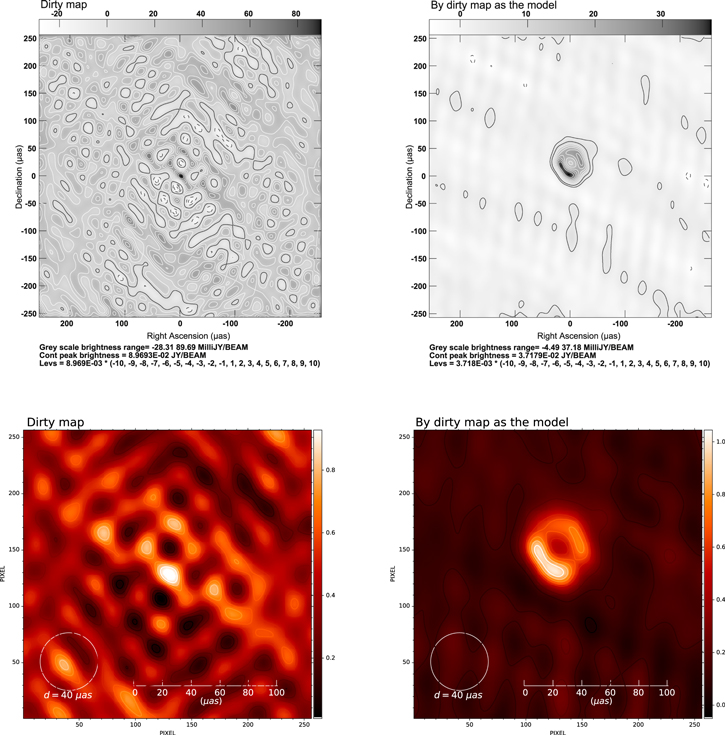
Figure 20. Ring image obtained using the dirty map. The left panels show the dirty map of the first day of data from the EHT observation. The right panels show the image resulting from self-calibration of the central part of the dirty map as an image model. The upper panels show a larger area of 500 μas width, and the lower panels show the enlargements of the central part of the images.
Download figure:
Standard image High-resolution imageThis is not a blurred intrinsic image of M87, but a strong reflection of the substructure in the dirty beam (PSF) of the EHT array. Figure 21 shows the dirty map and the dirty beam. Not surprisingly, they agree rather well, and that means the central ring-like structure we showed in Figure 21 is just the reflection of the shape of the dirty beam and not a physical reality. If we were to believe there should be a ring, it would be very natural to select the partial image from what looks like a ring in the dirty map. If we do so, what will happen? To answer this question, we tried the calibration of phase and amplitude using this ring-like structure at the center as the image model. We calculated the amount of calibration of the amplitude and phase by the self-calibration method. After the calibration is applied, we made an image using the CLEAN algorithm assuming that the source is single and compact. Here, the CLEAN subtraction area is limited by a circle with 30 μas radii centered at (+2 μas, +22 μas) from the map center, which is the BOX setting as used in the EHTC-DIFMAP pipeline (Section 5.5).
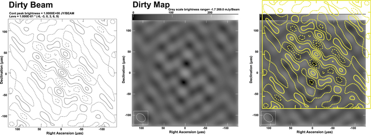
Figure 21. Comparison of the dirty beam (PSF) and the dirty map. The left panel shows the dirty beam (PSF), and the center panel shows the dirty map. The right panel shows a case where the two images were adjusted to fit well together and overlap. The yellow contours show the dirty beam, and the gray scale show the dirty map. The dirty beam (PSF) here is the same as shown in Figure 19, but the number of contours has been reduced. The dirty map here is the same as in the left panels of Figure 20, but the gray scale shows the intensity inversion image.
Download figure:
Standard image High-resolution imageThe obtained ring image is shown in the right panel of Figure 20. The size of the ring is close to that of the EHTC ring. What we would like to emphasize here is that in order to create a ring structure we need a narrow BOX setup. Without a narrow BOX, a ring structure cannot be created. If we change the position or size of the BOX, the ring deforms. When we use BOX offset setting of 22 μas from the center, we get a ring very similar to the EHTC ring. In other words, the shape strongly depends on the location of the imaging region. As we will show in Section 5.4, the EHTC BOX setting limits the FOV so narrowly that it can produce the EHTC ∼40 μas ring shape even from simulated data that does not contain the ring shape.
Close inspection reveals that the ring-like structure of the dirty map is at an offset position from the center. Since the structure of the PSF always shows central symmetry, one might think that the offset ring-like structure is not due to the PSF, but really exists at the offset position. However, the shape of Figure 3 shows that this is not the case. Figure 3 shows the structure of the CLEAN map after deconvolution from only the brightest point at the center of the dirty map. There is no ring-like structure here. We can see that the ring-like structure of the dirty map (Figure 20) is created by convolution of the dirty beam to the brightest point in the center. The ring-like structure is offset because the true source image inherent in the data does indeed exhibit noncenter symmetry it, however, is not an offset ring, but a core-knot structure as shown in Figure 7.
5.4. Ring from the Simulated Data of Different Structures
In this section, we demonstrate that, with the u−v coverage of EHT for M87, one could “observe” a ring even if the physical sources have different structures. As the physical source structure, we consider a single point with flux density of 1 Jy at the center. We made the simulated visibility data by applying the Fourier transformation to the single point image (We used UVMOD, a task in AIPS.). The u−v coverage is exactly the same as that of EHT for M87 observations. As for the noise, we consider two cases, one with relatively large noise (case 1) and the other with no noise (case 2). For case 1, we added thermal noise. The noise level is proportional to the weight of each data noted in original FITS public data. The S/N is 0.01 on average. We then perform experiments of calibration and imaging. For calibration, we obtain solutions from self-calibration with incorrect image models that are different from the true structures of the source, then apply the solutions to the data. We inspect what kinds of images appear from CLEAN imaging. For the self-calibration, we assume models of two incorrect images. One is the EHTC ring image (model A), and the other is a pair of two points separated by 45 μas (model B). Model B is a pair of points of 0.5 Jy located at (0 μas, 0 μas) and (0 μas, +45 μas) respectively. The locations of these two points roughly correspond to the positions of the main peak and the first sidelobe peak in dirty beam. We get calibration solutions of amplitude and phase from the self-calibrations (we used CALIB, a task in AIPS.).
By using IMAGR, a task in AIPS, we performed the CLEAN imagings. We limit the CLEAN subtraction area by a narrow BOX setting; a circle with 30 μas radii centered at (+2 μas, +22 μas) from the map center, which is a mimic BOX setting as used in the EHTC-DIFMAP pipeline (Section 5.5). The left panel in Figure 22 shows the ring image obtained from the large noise data (case 1). The obtained image from CLEAN is identical to the model image A used in self-calibration. When the S/N is very low, the CLEAN image after self-calibration can be identical to the model image used. Therefore, the result of case 1 does not tell much.
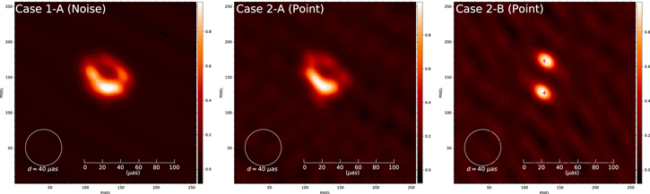
Figure 22. Resultant images from the simulated data sets. Case 1-A (left panel) shows the ring shape created from nearly noise data set, after applying the solution by self-calibration using the EHTC ring as the image model. Case 2-A (middle panel) shows the ring shape created from a single point data set with infinite S/N (no noise), after applying the solution by self-calibration using the EHTC ring as the image model. Case 2-B (right panel) is a two-point image created by applying the solution by self-calibration with two points as image models to a single point data (no noise data) with infinite S/N. The two red crosses indicate the positions of the points in the model image used in self-calibration.
Download figure:
Standard image High-resolution imageThe results of case 2 are surprising. The middle panel in Figure 22 shows the ring image obtained from no noise data. The obtained image from CLEAN is very close to the model image A used in self-calibration. Even when there is no noise, if we start with the assumption that there is a ring in the self-calibration image model, with the u−v coverage of EHT, we obtain a ring similar to that obtained by the EHTC.
The right panel in Figure 22 shows the result of using model image B for self-calibration. Though we used the data of a single point with no noise, we obtained a two-point image, which is very close to model B used in self-calibration. In addition, the two points appearing show small shifts from the positions in model B. The center point shifted toward the east, while the upper point shifted toward the west. These shifts seem to be the influence of the structure of the dirty beam. The shift of the center point is along the ridge elongated from the main beam in the dirty beam, while the shift of the upper point is toward the peak position of the first sidelobe.
The results of these experiments show that the reproduced images are very close to the image model used in the self-calibration. Such a result does not occur when the u−v coverage is sufficient, as in the case of VLA and ALMA. Unfortunately, the u−v coverage of EHT is not sufficient, and it has a special bias that makes it prone to producing shapes (including rings) with a size of ∼40 μas. We have shown that the shape of the PSF (essentially the effect of the sampling bias that makes it easy to create ∼40 μas structures) has the power to create ∼40 μas ring structures even from data with only one central point structure (centrosymmetry). However, the most powerful factor is not the data correction by self-calibration with wrong model images. Here and in Section 5.3, we showed that the very narrow FOV setting of the BOX has great power to create a ∼40 μas ring structure. In Section 5.5, we will discuss the setting of BOX in the EHT-DIFMAP pipeline.
5.5. What the EHTC Really Did in Their DIFMAP Imaging Process
In this section, we investigate the data processing pipeline that the EHTC used for imaging the EHTC ring with DIFMAP. 16 Among the three methods the EHTC used for the imaging, DIFMAP is the closest to the usual procedure 17 in the above web page. The other two are rather new, and difficult to study here. Since all three methods gave essentially the same image, we believe it is sufficient to analyze one of the three methods to find out why the ring structure was formed. The EHTC-DIFMAP imaging analysis used the hybrid mapping technique to calibrate the data and obtained the image. The hybrid mapping method is the standard method of VLBI calibration and imaging.
Let us first summarize the standard procedure of VLBI data calibration and imaging. The radio interferometer samples the spatial Fourier components of the brightness distribution of the observed source (often called visibility). Theoretically, the brightness distribution of the observed source can be obtained by collecting the samples and performing the inverse Fourier transform. However, there are actually two problems as follows. (a) The sampled visibility data contain errors, so they are not the correct spatial Fourier components. Therefore, it is necessary to calibrate them. Self-calibration is a method of obtaining calibration solutions by using an assumed image. If the assumed image is not correct, the correct calibration solution cannot be obtained. (b) The number of observed samples is limited. The inverse Fourier transform alone does not produce the correct image. The PSF does not become a point. Therefore, the PSF shape must be deconvolved. For this purpose, image processing is performed. As a method to obtain the correct calibration solutions and to attain clear imaging results, hybrid mapping, which alternates between the above two tasks, is usually used in VLBI imaging. We use self-calibration for calculating the calibration solution using a tentative image model, and CLEAN for performing deconvolution of the scattered PSF shape.
Hybrid mapping is the following algorithm. (a) Assume an image model for self-calibration. For the first one, a one-point model is usually used. (b) Calculate tentative calibration solutions from self-calibration using the image model. (c) Calibrate visibility data using the tentative calibration solutions. (d) Obtain the next tentative image using CLEAN from the calibrated visibility data. CLEAN image is composed of point sources (CLEAN components). (e) Make the next image model for self-calibration by picking up reliable CLEAN components from the image. (f) Go back to (b) and repeat the iteration from (b) to (e) until a satisfactory image is obtained.
The visibility (spatial Fourier component) is a complex quantity, and so it has amplitude and phase. It is safe first to repeat self-calibrations only for phase solutions until a nearly satisfactory image is obtained and to perform self-calibration for amplitude and phase by using that image. This is because self-calibration for amplitude tends to give a solution that is too close to the model image used in self-calibration (Cornwell & Fomalont 1999).
However, the repetition of amplitude self-calibration is often performed under the careful check of the practical quality of the data, and then, in many cases, good calibration solutions can be obtained.
In addition, the BOX technique is an auxiliary means used for imaging with CLEAN. (It is essentially unrelated to the hybrid mapping method.) We can limit the area of CLEAN subtraction intentionally by the BOX setting. This technique may give us a good image, even when the calibration is incomplete. As already mentioned, we used the BOX technique in our analysis. The EHTC-DIFMAP analysis did the same.
Now we investigate the EHTC-DIFMAP procedure. The EHTC-DIFMAP imaging analysis performed the self-calibration only for phase solutions with a single point-source model, following the general procedure of the hybrid mapping method. However, after the first phase self-calibration, they used the BOX technique with a very narrow BOX 18 in the first imaging trial. The CLEAN subtraction area was restricted to within the circle of 60 μas diameter specified by the BOX.
The BOX is roughly a circle of diameter 60 μas composed of 30 small rectangles. By comparing the BOX shape and the dirty beam, we found that the BOX covers the main beam and the first sidelobe, but leaves out the second and other sidelobes. The BOX is not located at the phase center but offset by +22 μas in the y-direction (δ direction). This offset of 22 μas coincides with the radius of the EHTC ring. Figure 23 shows the EHTC BOX position on the dirty beam (PSF) aligned by their phase centers. The area of the EHTC BOX covers (1) the main beam peak, (2) the ridge extending to the left (east) from the main beam peak, (3) a part of the first sidelobe located north of the main beam, and (4) an area of negative strength near the center of the box area. The structure of the dirty beam within the EHTC BOX is close to the shape of the EHTC ∼40 μas ring.
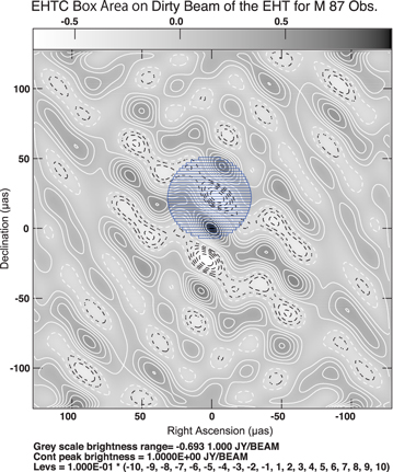
Figure 23. The size and position of the BOX used in their DIFMAP pipeline (blue shaded area). We overlaid the BOX on the dirty beam (PSF), which is already shown in Figure 19. We align the two figures at their phase centers.
Download figure:
Standard image High-resolution imageThe PSF structure within the BOX explains not only the diameter of the EHTC ring, which is ∼40 μas, but also the asymmetric structure of the EHTC ring. The EHTC ring has an asymmetric structure with a bright south side. The brighter south side corresponds to the main beam (the brightest in the box), while the darker north side of the ring corresponds to the first sidelobe in the north (the less bright peak in the box).
If such a narrow BOX with the offset is used from the beginning to the end of the hybrid mapping process, the effect of the dirty beam can be enhanced as we showed in Section 5.3. It is quite clear that the EHTC ∼40 μas ring is the result of such enhancement of ∼40 μas substructures in PSF.
We actually ran the EHTC-DIFMAP pipeline to investigate its behavior and performance. The left panel of Figure 24 shows the resultant ring image from running the EHTC-DIFMAP pipeline with the default parameter settings. On the other hand, the right panel of Figure 24 shows the image obtained by removing the BOX setting (Figure 23) from the EHTC-DIFMAP pipeline. The ring in the BOX setting region has been destroyed, and the brightness distribution has been extended to outside the BOX setting region. The new brightness distribution shows a core-knot structure in the center, similar to the results of our analysis. In addition, several emission peaks appear in the PA = 45° and PA = 225° directions from the center. These are probably sidelobes, but it is very interesting that one emission peak in the PA = 225° direction corresponds to the feature W we found in our analysis. This result implies that the very narrow BOX setting of the EHTC-DIFMAP pipeline is the main factor that creates the EHTC ring image.
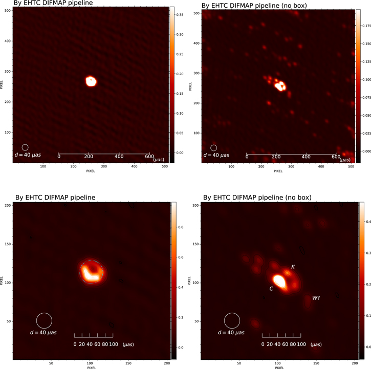
Figure 24. Resultant images from the EHTC-DIFMAP pipeline. The upper panels show the entire field of view with the default setting of the EHTC-DIFMAP pipeline (1 mas square). The lower panels show the enlargement of the central part of the upper images. The left panels show the result of running the EHTC-DIFMAP pipeline with the default parameter settings. The light blue circle shows the location and size of the BOX. The ring-shaped image appears in the BOX area. The right panels show the resulting image when the EHTC-DIFMAP pipeline is run without the BOX setting. In the enlarged image (bottom right), we can see the emission peaks corresponding to the three components we found: core (C), knots (K), and west component (W). Here, we used the data named SR1_M87_2017_095_hi_hops_netcal_StokesI.uvfits.
Download figure:
Standard image High-resolution imageWe also created simulated data and applied the EHTC-DIFMAP pipeline to it to investigate what kind of images are obtained. The purpose of this is to check if the EHTC-DIFMAP pipeline always calibrates the data correctly and reproduces the true picture of the data. We created simulated data with the task UVMOD in AIPS and acquired images with both the task IMAGR in AIPS and the EHTC-DIFMAP pipeline for comparison. Figure 25 shows examples of the simulation results. Three cases are shown: (1) a core-knot model aligned in about PA = −38°.7 direction (left panels), (2) a two-point model aligned in north–south direction (center panels), and (3) a 40 μas diameter ring, but the ring width is 2 μas, which is different from that of the EHTC ring (right panels).
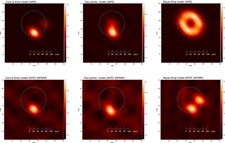
Figure 25. Resulting images of simulation data. The upper panels show the imaging results when using IMAGR in AIPS. The lower panels show the imaging results when using the EHTC-DIFMAP pipeline with default parameter settings. The same BOX setting is used for IMAGR as well as the EHTC-DIFMAP pipeline. The light blue circles show the position and size of the BOX setting. The three results are presented. A core-knot model (left panel), a two-point model (center panel), and a ∼40 μas ring model (right panel). The red crosses on the left and in the center indicate the positions of the emission points placed during the simulation data preparation.
Download figure:
Standard image High-resolution imageThe top panels show images obtained from data simulated using the AIPS IMAGR task with the same box settings as the EHTC-DIFMAP pipeline. The IMAGR produced the expected image.
The bottom panels of Figure 25 show the results of the EHTC-DIFMAP pipeline. The original images of the simulated data could not be reproduced. In the case of the core-knot model (lower left panel), the knot component is lost. Also, in the case of the two-point model (bottom center), the weak north point has disappeared. Even more surprisingly, in the case of the 40 μas diameter ring model (bottom right panel), the image quality is degraded and the ring structure is obscured.
Since these images are compact and fit within the BOX setting of the EHTC-DIFMAP pipeline, this phenomenon is not due to a narrow FOV caused by the BOX setting. This is probably because the performance of the hybrid mapping process of the EHTC-DIFMAP pipeline strongly depends on the image structure and noise structure of the input data.
Note that we have performed many simulations and what are shown in Figure 25 are selected samples. The summary of our simulations is as follows.
- 1.A single point-source model of 1 Jy with no noise. The image was reproduced from both IMAGR in AIPS and the EHTC-DIFMAP pipeline.
- 2.Complete noise model. No specific image was detected from the IMAGR in AIPS, but a single point was obtained from the EHTC-DIFMAP pipeline. This is probably due to the fact that the first self-calibration was performed using the image model of a single point source. This is a common phenomenon that occurs when self-calibration is applied to data sets with very low S/N.
- 3.Core-knot model. Two-points model consisting of a point of 1 Jy at the center (0 μas, 0 μas) and a point of 0.25 Jy at (−25 μas, +20 μas). The distance between them is about 32 μas, and they are located along a line in the direction PA = −38°.7. 12 simulation data with noise ranging from zero to 640 Jy/weight were generated. IMAGR in AIPS detected the core-knot structure as expected. In the EHTC-DIFMAP pipeline, the knot component disappeared in 11 of the 12 cases.
- 4.Ring images with diameters around 40 μas. The ring width is 2 μas, and the ring diameters are 30, 35, 40, and 45 μas. The flux density of the image is 1 Jy. No noise was added. Using IMAGR in AIPS, the hole in the center of the ring is obscured when the ring diameter is smaller than 30 μas. When the ring diameter is larger, the ring can be recognized. On the other hand, using the EHTC-DIFMAP pipeline, the structure of the ring became ambiguous in all images, like the example shown in Figure 25.
- 5.Two-point model (shift in the north–south direction). Place a point of 1 Jy at the center (0, 0 μas) and a point of 0.5 Jy north of it. There are 11 intervals: 0, 5, 10, 15, 20, 25, 30, 35, 40, 45, and 50 μas. Using IMAGR in AIPS, two points cannot be separated and resolved when the spacing is very narrow. At a separation of 10 μas, the image is elongated in the north–south direction. If the separation is larger than 25 μas, the two points are reproduced separately. Using the EHTC-DIFMAP pipeline, when the separation is larger than 45 μas, the two points are reproduced correctly, but otherwise the north point is not reproduced in the correct position.
- 6.Two-point model (east–west shift). A point of 1 Jy is placed at the center (0 μas, 0 μas), and a point 0.5 Jy is placed at δ = 42 μas. The R.A. position of the second point is shifted every 5 μas from −20 to 20 μas to create 9 simulation data. The positions of these two points are reproduced from IMAGR in AIPS. The EHTC-DIFMAP pipeline reproduces these two points in four cases. In the other four cases, the position of the north point deviated from the correct position by more than 10 μas.
Thus, in most cases, the EHTC-DIFMAP pipeline did not reproduce the intrinsic image of the simulation data. Figure 10 of The Event Horizon Telescope Collaboration et al. (2019d) shows that their procedure successfully reproduces images from simulated data (ring, crescent, disk, and double source), but their results are inconsistent with ours (at least for the EHT DIFMAP case). In our simulations, noise is either not added at all or, if added, it is thermal noise. IMAGR in AIPS reproduces the input model images reasonably well, while the EHTC-DIFMAP pipeline does not. The difference between the two methods is the hybrid mapping process. The EHTC-DIFMAP pipeline lacks the performance of the general calibration of the data described in Section 5.8.3.
5.6. The Amounts of Calibrations Performed in the EHTC Imaging Process
The EHTC papers give the detailed description of the data calibrations at the early stage process, but not much about the calibrations performed during the imaging process (through the self-calibration in the hybrid mapping process of the EHTC-DIFMAP imaging analysis case). This is an insufficient description of data calibrations because it is rare that only a-priori calbrations are sufficient for obtaining VLBI fine images. We, therefore, estimate and show the amounts of calibrations performed by the EHTC during their imaging process. We attempted to reconstruct them in the following procedure. First, following the EHTC open procedure, we reproduced the EHTC ring image of the first observing day (the left panel in Figure 26). Then, using the CLEAN components of the ring image as the model image, we performed self-calibration by the task CALIB in AIPS and got solutions for both the phase and amplitude. The parameters of CALIB are shown in Table 6. In Figures 27 and 28, we show the total amount of calibrations both of phase and amplitude in the case of the EHTC ring image model. Note that we performed CLEAN imaging to verify if the solutions from the self-calibrations are consistent with the original the EHTC ring image. First, we flagged out data points where the amplitude solutions were more than 4 by using the task SNCOR in AIPS. Here we followed the standard VLBI teaching, which states that “discarding bad data will make a better image than keeping them.” Then, we applied the solutions to the selected data and obtained an image using the task IMAGR in AIPS for CLEAN. The right panel of Figure 26 shows the resultant image whose quality is similar to that of the original EHTC ring. Thus, our solutions of self-calibrations successfully reproduced the EHTC ring image.
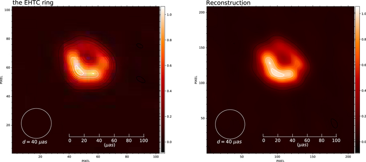
Figure 26. Left panel shows the EHTC ring image of the first day observations. We obtained this image by using their open procedure. The right panel shows our reconstruction image by applying the self-calibration solutions shown in Figures 27 and 28. The same BOX setting as that used in the EHTC-DIFMAP pipeline was used. Also the same restoring beam was applied (23.1 × 17.0 μas with PA = 44°.4).
Download figure:
Standard image High-resolution image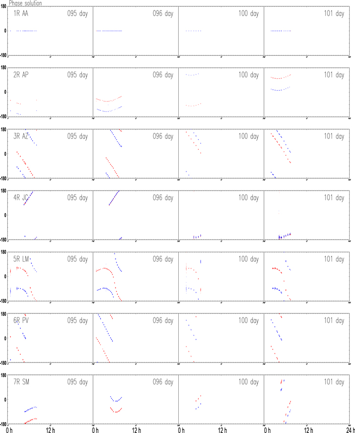
Figure 27. Phase solutions obtained from self-calibration using the EHTC ring image. The red points show the solutions for IF 1 data; the blue ones show those for IF 2 data.
Download figure:
Standard image High-resolution imageTable 6. Parameters of CALIB for the Amplitude and Phase Self-calibration
| SOLTYPE | “L1” |
| SOLMODE | “A&P” (both phase and amplitude) |
| REFANT | 1 (ALMA) |
| SOLINT (solution interval) | 0.15 (minute) |
| APARM(1) | 1 |
| APARM(7) (S/N cutoff) | 3 |
Download table as: ASCIITypeset image
The phase and amplitude solutions for the EHTC ring image are very similar to, or worse than our results in Figures 5 and 6. Therefore, if such large amplitudes and their rapid variations found in the self-calibration solutions are negative signs against the resultant image quality, both the results of our final images and the EHTC ring images should be rejected. This implies that the “calibrated” data released by the EHTC are not of high quality (as is often the case with VLBI archival data).
5.7. Sensitivity of the ∼40 μas Ring to BOX Size
In Section 5.6, we reproduced the ring structure obtained by the EHTC, by using the very narrow box used by the EHTC. If the ring image is definitely correct, it should only weakly depend on the BOX size. In fact, we studied the effect of changing the BOX in Section 4.3.2, and found that the main structure of our final image (features C & K) does not disappear. In this section, we investigate the sensitivity of the ring structure obtained by the EHTC to that from the BOX method they used.
We calibrated the data by applying the calibration solutions obtained from the self-calibration using the EHTC ring as the image model, which are shown in Figures 27 and 28. We performed CLEANs using BOXes of circles with diameters of (a) 60 μas, (b) 80 μas, (c) 100 μas, (d) 120 μas, (e) 240 μas, and (f) 450 μas. Their centers are located at the same position as that of the EHTC-DIFMAP pipeline case. Other parameters of the CLEANs are the same as those used for the right image in Figure 26.
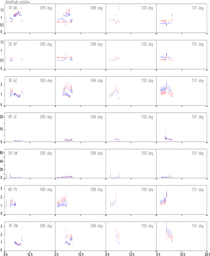
Figure 28. Amplitude solutions obtained from self-calibration using the EHTC ring image. The red points show the solutions for IF 1 data; the blue ones show those for IF 2 data.
Download figure:
Standard image High-resolution imageThe results are shown in Figures 29 and 30. Figure 29 shows views of the entire imaging area of 2 mas square, and Figure 30 shows enlarged views of the central 256 μas square. The BOXes used are indicated by blue circles. The ring structure in panel (a) (D = 60 μas) is the same as that in the right panel of Figure 26. Here, we can see the ring structure similar to that obtained by the EHTC. The ring extends beyond the BOX area. This is because the obtained CLEAN components are near the boundary of the BOX, and a 20 μas restoring beam is convolved to form the CLEAN map. In the cases of (b) D = 80 μas and (c) D = 100 μas, the ring is still recognizable. However, we can see CLEAN components not on the ring but near the boundary of the BOX when the BOX becomes larger. In the case of (d) D = 120 μas, there are several CLEAN components almost on the boundary of the BOX; though the ring structure is still recognizable. In the cases of (e) D = 240 μas and (f) D = 450 μas, there is no ring. Instead, one elongated bright spot appears. We also tried larger BOX cases, D = 900 μas, and D = 1300 μas, and the resulted image is similar to the case of D = 450 μas. They show a bright spot at the center of the map.
Figure 29. Stability of the EHTC ring structure against the BOX sizes: the whole 2 mas square images of the CLEAN results by IMAGR (AIPS). Panels (a)—(f) show the resultant images in cases of expanding the diameter of the BOX area with D = 60, 80, 100, 120, 240, and 450 μas respectively. The blue circle shows the respective BOX area. The center positions of the circles are (−2 μas, +22 μas) as following the BOX the EHTC-DIFMAP analysis.
Download figure:
Standard image High-resolution image
Figure 30. Stability of the EHTC ring structure against the BOX sizes: the enlarged views of the central 256 μas square from the resultant CLEAN images by IMAGR (AIPS). Panels (a)—(f) show the resultant images in cases of expanding the diameter of the BOX area with D = 60, 80, 100, 120, 240, and 450 μas respectively. The blue circle shows the respective BOX area. The center positions of the circles are (−2μas, +22 μas), as following the BOX the EHTC-DIFMAP analysis.
Download figure:
Standard image High-resolution imageIf the FOV is smaller than that for the case (d), a ring image will appear, and if FOV is larger than that, the ring image will be destroyed. In other words, the boundary FOV is around 120 μas. It is an odd coincidence that the EHTC imaging analysis set the FOV to be 128 μas (The Event Horizon Telescope Collaboration et al. 2019d), just around the boundary FOV. (It is 60 μas in the case of the EHTC-DIFMAP pipeline as already mentioned.) 19
Thus, we can conclude that the EHTC ring appears only when a very narrow BOX is applied.
5.8. Problems in the EHTC Analysis
Here we explain why the EHTC created the image of the ring. The EHTC described the details of their imaging process in The Event Horizon Telescope Collaboration et al. (2019d), in which we found some of the reasons why they created an artifact. The EHTC conducted various surveys, but their methods were not objective and were biased from the very beginning of their analysis.
5.8.1. Attention to Sampling Bias
It is well known that the sampling bias in data can seriously affect data analysis. For the sampling bias, two things should have been done.
First, PSF (dirty beam) structure should have been checked. In radio interferometer data analyses, checking the structure of the dirty beam usually provides insight into the effects of insufficient u−v coverage; in a sparse array configuration such as the EHT array, it is very important to check the shape of the dirty beam and utilize it to prevent false imaging. The Event Horizon Telescope Collaboration et al. (2019d) describes the size and shape of the main beam of the dirty beam and the corresponding CLEAN beam, but we do not find any discussion of the overall dirty beam structure in the EHTC paper. As already shown, the separations between the main beam and the first sidelobes of the dirty beam structure are ∼40 μas, which coincidentally is the same as the expected size of the black hole shadow in M87.
Second, performance of the new imaging method with respect to the sampling bias needs to be verified. The CLEAN algorithm, the well-known imaging method in radio interferometry, was originally designed to obtain correct images by deconvolving the false structures appearing in dirty beams (the origin of which is the sampling bias). However, in actual use, it is not easy to completely eliminate this effect; the CLEAN method’s performance against the sampling bias and residual structure due to the bias is known from its long history of use.
5.8.2. The EHTC Simulations
The EHTC conducted simulations to find the optimal parameters for imaging. According to The Event Horizon Telescope Collaboration et al. (2019d), “In the second stage [the EHTC] reconstructed synthetic data from a large survey of imaging parameters and then compared the results with the corresponding ground truth images. This stage allowed us to select parameters objectively to use when reconstructing images of M87.” However, there are two major problems with this simulation.
First, it seems that the idea of what to be obtained from the simulation was not well considered: the EHTC created synthetic data from the model images and searched for optimal parameters to reproduce the input model images. But what the EHTC should be obtaining here is a parameter that can correctly calibrate the data and then reconstruct the image correctly. In their simulations, it seems that no attention was paid to the reproducibility of the input error model. Optimal parameters are those that need to be satisfied not only for the reproduction of the input image model but also for the reproduction of the input error model. As mentioned before, the reproduction of the input image model can be due to the sampling bias. In order to reject this possibility, it is useful to check whether the input error model is also reproduced simultaneously.
We tested the performance of the EHTC-DIFMAP with images of similar size to the EHTC image model and found that most of the images were not reproduced correctly (Section 5.5). The EHTC-DIFMAP parameter settings are of serious concern for the imaging performance of general images other than the EHTC’s four image models. We put thermal noise and/or no noise into our simulated visibility. From simple CLEAN by IMAGR in AIPS the input images are reproduced, while from the EHTC-DIFMAP pipeline, they are not reproduced correctly. It means that the EHTC optimal parameters have problems in their calibration performances. We could not find description of the reproducibility of the input model errors in the EHTC papers. The EHTC conducted vast amount of simulations to search for the optimal imaging parameters, but we worry that what was optimized was only the reproducibility of the input image model, not the input error model. They should have searched for a parameter that could reproduce not only the input model images but also the input model errors at the same time.
Second, the large-scale simulation of the EHTC was not so vast as to provide for optimal imaging of M87. The number of selected image models and the range of FOV settings are not sufficient for the purpose of the simulation. Therefore, the imaging method using their optimal parameters does not have the general performance of producing correct images. The following are some of the insufficient aspects of their parameter search.
- 1.The selected model images (geometric models). The following four central compact model images have been adopted (The Event Horizon Telescope Collaboration et al. 2019d): (1) ring: a delta-function ring with radius r0 = 22 μas, convolved with a circular Gaussian with FWHM of 10 μas; (2) crescent: crescent composed of a delta-function ring with radius r0 = 22 μas and a dipolar angular intensity profile; (3) disk: a uniform disk with radius r = 35 μas, convolved with a circular Gaussian with FWHM of 10 μas; (4) double: two circular Gaussian components, each with a FWHM of 20 μas. The first component is located at the origin and has a total flux density of 0.27 Jy, while the second is located at ΔR.A. = 30 μas and Δdecl. = −12 μas and has a total flux density of 0.33 Jy. These image models were selected based on a plot of visibility amplitude versus u−v distance (Figure 2 in The Event Horizon Telescope Collaboration et al. 2019d). The EHTC claimed that they found two null points in this plot, at ∼3.4 and ∼8.3 Gλ, and identified them as important marks for selecting image models including a ring model. In the EHTC plot of amplitude versus u−v distance, there appear to be two null points, but it should be noted that the amplitude axis is logarithmic. It means that the null level (amplitude = 0) is not shown in the plot area. It might, naturally, be a good choice to adopt the minimum detection sensitivity as the de facto null level. The EHTC papers did not describe the detection sensitivity in detail, but according to The Event Horizon Telescope Collaboration et al. (2019b), the characteristic sensitivity is 1 mJy for ALMA connected baselines and 10 mJy for other baselines without ALMA. The lower limits of their amplitudes of the plots are set slightly higher than these characteristic sensitivity levels. 20 Therefore, the existences of the two null points are not obvious.In the old days of VLBI observations, when synthesis imaging was not available, such plots were the only way to get a rough estimate of the structure of the observed source. One must be aware that there are numerous candidates that satisfy the visibility amplitude plot. Therefore, in principle, it is not possible to identify a unique structure from the plot. In the EHTC simulations, only four image models were selected, which seems insufficient to search for optimal imaging and calibration parameters.Furthermore, as can be seen from the attached error bars, this amplitude measurement contains considerable ambiguity. Also, as shown in Sections 3.5 and 5.6, the amplitude values before the final calibration contain large errors that cannot be neglected. In particular,for interferometers consisting of antennas of various aperture sizes, comparing the amplitudes of individual baselines tends to be confusing. Therefore, image estimation from such amplitude plots should be done with a large uncertainty in mind. Since the error is not small, it cannot be easily determined to be a null point, and even if it is, its exact location is not clear. Therefore, it is not possible to select definitive image models based on a strong recognition of this null point.Here we raise another serious concern: of the four image models, two have structures with a diameter of 44 μas. This diameter corresponds to the size of the false structure that can be caused by the sampling bias. Their optimal imaging parameters are likely to be rather optimized to increase the sampling bias effect.
- 2.Consideration in large-scale jet model. In addition to the compact image model, the EHTC has added an image model for the large-scale jet. The EHTC has adopted three Gaussian shapes as the jet model, based on the results of the previous study of 86 GHz observations (Kim et al. 2018). The largest Gaussian has a size of 1000 × 600 μas, and the other two have a size of 400 × 200 μas. They hoped that these would mimic the structure surrounding the core and the jet flow with both edges brightened. However, this choice of jet model does not seem to be a good model for VLBI observations at 230 GHz.First, the size of the model jets is too large to simulate observations at 230 GHz. It is not appropriate to use the results of 86 GHz observations; the jets observed at 86 GHz are blurred due to the lower spatial resolution and do not show the intrinsic size at 230 GHz. The intrinsic size is probably much smaller. We can expect to detect a smaller jet component at 230 GHz because of the higher spatial resolution. Second, the EHT imaging performance does not have sufficient power to detect large, smoothed structures (such as Gaussian shapes). According to our EHT array performance simulations (Appendix A), the detectable size is less than 15 μas. Let us explain what is actually done in this EHTC simulation with the jet model. This simulation result only says that the large, smooth jet structure does not have any effect on the imaging of the compact structure of the core. Here, it is very important to note that the simulation is limited to “large, smooth structure.” If the jet consists of compact features as found in our imaging, their simulation cannot rule out the effect of jet features to the image of the core created using a small BOX size. Our imaging results (Section 4.2) show that the jet structure is composed of a cluster of small features, which means that the EHTC simulation was performed with an unrealistic assumption.
- 3.The FOV setting. “The choice of FOV must be made with care, as incorrect restrictions can result in false image structure” (page 4 in The Event Horizon Telescope Collaboration et al. 2019d)—which is really a very important point. The EHTC set the FOV to less than 128 μas. As we have shown in Section 4, the actual image extends further out of the FOV size. Also, as shown in Section 5.7, there is a critical FOV size of around 128 μas. If the FOV is larger than that, the image of the ∼40 μas ring is destroyed, and if the FOV is smaller, the image of the ∼40 μas ring is enhanced. The optimal FOV selected by the EHTC coincides with the critical FOV required to create ∼40 μas ring artifact.M87 is a very important target for the study of the jet structure of AGN. Therefore, previous VLBI observations have mainly pursued the investigation of its jet structure. In 2017, the EHT array achieved unprecedented sensitivity, and thus we naturally expected that it would detect weak emission belonging to jet structures that were not detected in previous EHT observations (without ALMA). A wide FOV had to be set to take the jet detection into account.
The EHTC selected their optimal parameters based only on the reproducibility of the image models in simulations. Nothing was written about the reproducibility of the input error models; probably the reproducibility of the input error models was not taken into account. Both reproducibilities should be examined when selecting the optimal parameters for data calibration and imaging. This would help to detect the false imaging due to the effects of data sampling bias.
5.9. The Reasons Why the EHTC Obtained the Artifact Image
We here summarize the reasons why the EHTC obtained the artifact image unintentionally. The fundamental reason is the sampling bias in EHT’s u−v coverage for M87, i.e., the missing ∼40 μas spatial Fourier components (Section 5.1). The sampling bias tends to create an artificial structure of ∼40 μas in imaging. We confirmed that the artificial ∼40 μas sized structures appear in the dirty beams (PSF; Section 5.2, Appendix B) and in our CLEAN imaging results (Appendix C).
The CLEAN algorithm was originally designed to remove false structures such as sidelobes that appear in PSF, but it does not always succeed in doing so. Also, other imaging methods of the EHTC, if no special countermeasures are taken against u−v sampling bias, will produce artificial structures in the imaging results with sizes of ∼40 μas of the sampling bias origin. In addition, the u−v sampling bias effects are independent of the need for data calibration. Therefore, even with the imaging methods based on observables that are free from systematic errors such as closure phase, we have no choice but to be aware of the effects. The sampling bias effect does not produce serious errors if careful data analysis is performed. However, the EHTC expected a ring-like structure of ∼40 μas in size from the beginning, and thus performed the image synthesis with a very narrow FOV (128 μas in size). A large FOV setting will not enhance the artificial ring image of ∼40 μas size. On the other hand, the very small FOV set by the EHTC enhances the sampling bias effect to create the ∼40 μas ring structure (Section 5.7). There were large amplitude errors in the observed data possibly originating from atmospheric variations (Section 3.5). This could have played a role in the initial analysis of the EHTC.
We would like to dedicate this work to an emeritus professor Yoshiharu Eriguchi of the Tokyo University and Dr. Jose Ishituka in Peru (both passed away in 2020), also to a professor Naruhisa Takato of SUBARU observatory in Hawaii (passed away in 2021). We thank Jun Fukue, Hiroyuki Takahashi, Hisaaki Shinkai, Hiroshi Imai, Hiroshi Sudou, Masao Saito, Hiromi Saida, Yasusada Nanbu, and Masaaki Takahashi for their kind comments. Takahiro Tsutsumi and Shunya Takekawa kindly provided new tools for checking the data.
Facility: EHT. -
Appendix A: Imaging Simulations for Investigating the u−v Performance of the EHT Array
In VLBI imaging with sparse u−v coverage, sometimes the reconstructed images do not show the real brightness distribution correctly. In particular, when the size of the source is significantly larger than that of the synthesized beam, the source image disappears, namely resolved-out occurs. Here, we investigated such an effect for the EHT u−v coverage for the M87 observations.
Figure 31 shows the simulation results for the reconstruction of Gaussian brightness distributions using the EHT array configuration. We used the model images of circular Gaussian shapes with a total flux density of 1 Jy. The sizes are 500, 250, 125, 62.5, 30, 15, 7.5, 5, and 2.5 μas in FWHM (the left panels in Figure 31). Here, we assume that the EHT array has an infinite sensitivity and that the data calibration is perfect; that is, we did not add any thermal and systematic noise error into the simulated visibility data.
Figure 31. u−v simulations using circular Gaussian shapes with various FWHMs. Larger structures than that of FWHM = 30 μas cannot be detected by the EHT u−v coverage. The contour levels are 0.5%, 0.78%, 1.1%, 1.6%, 2.2%, 3.13%, 4.4%, 6.4%, 8.9%, 13.5%, 18%, 25%, 35%, 50%, 71%, and 99% of the peak.
Download figure:
Standard image High-resolution imageBy CLEAN, we obtained the corresponding reconstructed images, as shown in the right panels of Figure 31. When the model image sizes are larger (FWHM = 500, 250, 125, 62.5 μas), they are completely resolved-out and cannot be detected even with infinite sensitivity. In the case of FWHM = 30 μas, it was almost decomposed but was detected as a small dark spot. In other words, the brightness distribution that can be modeled as a Gaussian shape larger than 30 μas in FWHM cannot be detected by the EHT array configuration. Although the smaller sizes with FWHM = 15 μas or less can be detected, they are not correctly reproduced as the original Gaussian shapes. In addition, the reconstructed images show streaks running in the northeast–southwest direction at lower levels. This also reflects the shape of the dirty beam (PSF) produced by the space u−v coverage.
In conclusion, the detectable structure of M87 by the EHT array configuration is limited to less than 30 μas in size, which corresponds to 2.43 × 10⁻³ pc (500 au) or 4.2 RS. Any larger extended structure cannot be detected. We must consider the possibility of the existences of more extended structures.
Appendix B: Dirty Beam Shapes with Different Weightings
In synthesis imaging using a radio interferometer, the shape of the PSF (dirty beam) can be changed by adjusting the weighting of u−v points. The normal PSF shape when EHT observes M87 is shown in Figure 19, but here we show the famous PSF shapes often used in synthetic images, i.e., the uniform weighting case and the natural weighting case. These PSFs were obtained by changing the parameter ROBUST in AIPS. 21
Figure 32 shows them. We set ROBUST = −5 for uniform weighting, and ROBUST = + 5 for natural weighting. As a whole, the shapes of each are not similar. In particular, the shape of the main beam is different. 22 However, they both have the same spacing substructure of about 40–50 μas in common. In particular, the spacing between the main beam and the first sidelobe and the direction of the line connecting them, i.e., the position angle, are almost the same. This means that, even if the weights of the u−v points are adjusted, the effect of spatial Fourier components that were not sampled during the observation cannot be essentially removed.
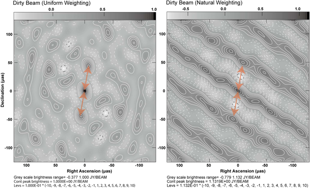
Figure 32. Other different dirty beam shapes (PSFs) of the EHT during the first day of observations of M87. The left panel shows the dirty beam shape by uniform weighting. The right panel shows that by natural weighting. Contour lines are shown in 10% increments from −100% to 100% of the peak. Positive levels are indicated by white lines and negative levels by dotted lines. The gray scale shows the range from the minimum to the maximum intensity of the dirty beam image. Both cases show that the first sidelobe levels reach more than 60% of the height of the main beam. As shown in Figure 19, red arrows with a length of 45 μas are placed at the same position and angle.
Download figure:
Standard image High-resolution imageAppendix C: Structure by the Sampling Bias in Our CLEAN Images
The EHT data sampling is biased in that the spatial Fourier components of ∼40 μas are missing. Because of this, the imaging results tend to contain false ∼40 μas -sized structures that do not actually exist. In our images, which were obtained by independently analyzing the same EHT data, there is no ∼40 μas size ring, but the effect of data sampling bias could still appear. Here, we investigate the spatial distribution of the CLEAN components in one of the CLEAN maps obtained from the hybrid mapping process and found the effect of data sampling bias. The CLEAN algorithm, assuming that the observed structure consists of a large number of point sources, finds the points from the visibility data. Accordingly, the result of CLEAN is obtained as a set of CLEAN components (position and intensity). We examined the spacing distribution of all pairs of CLEAN components. Raw CLEAN components can be in the same position as other components. In such cases, we used CCMRG, an AIPS task, to merge the raw CLEAN components in the same position into one. The number of CLEAN components after merging is Ncc = 2579, and the number of pairs of them is Npair = 3234331.
Figures 33 and 34 show the distribution of spacings for all pairs of CLEAN components. The distance between a CLEAN component pair is divided by a certain interval d (μas), and the distribution of the remainders are shown in the figures. If there is no characteristic structure at interval d, the remainder distribution will be flat. The panels (a), (c), and (e) of Figure 33 show such cases. That is, the three cases of d = 40, 60, 80 μas show a flat distribution. Fine saw-tooth shapes appear in panel (c). This is due to the effect of the grid spacing during CLEAN imaging. In this case, d = 60 μas is divisible by the grid spacing (1.5 μas).
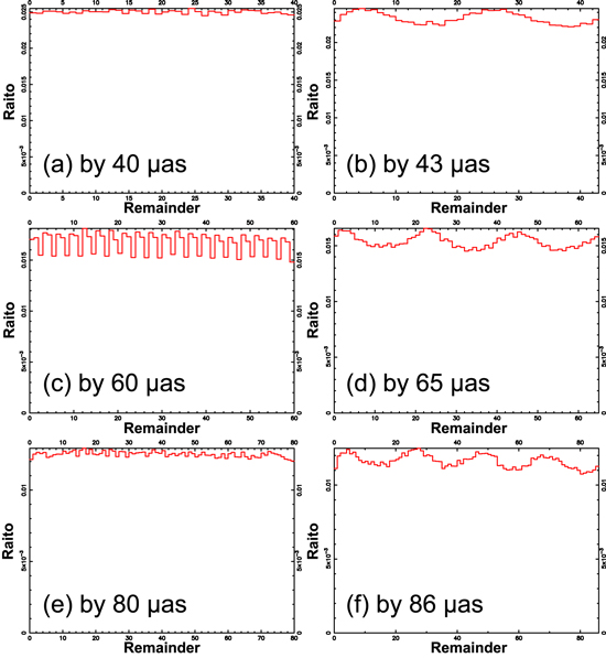
Figure 33. Histogram of intervals for CLEAN component pairs. The horizontal axis shows the remainder of the interval after dividing by d μas. The vertical axis shows the ratio of pairs in a bin. The width of the bin is 1 μas. Panel (a) shows d = 40 μas, (b) d = 43 μas, (c) d = 60 μas, (d) d = 65 μas, (e) d = 80 μas, and (f) d = 86 μas.
Download figure:
Standard image High-resolution imageHowever, at d = 43 μas, an arch shape appears and two peaks are formed. The spacing between these peaks is about 20 μas. A similar arch-like distribution is seen from d = 42.5 μas to d = 44.25 μas. For d = 65 (=43 × 1.5) μas, three arches can be seen. For d = 86 (=43 × 2) μas, four arches appear. Interestingly, the spacing between all the peaks is 20 μas. The position of these peaks is an integer multiple of 43 μas. This can be explained as the sum of the sampling bias effect and an integer multiple of the spatial resolution of the EHT array (20 μas). The first peak is not located at residual = 0 and shows a slight shift for d = 43 and 86 μas. The reason for this is difficult to explain.
Note that the basis of the characteristic interval is not d ∼ 20 μas, but d ∼ 43 μas. If the basis of the characteristic interval is 20 μas, then a single arche type shape should appear in the distribution for d ∼ 20 μas. As shown in Figure 34, the distributions for d ∼ 20 μas have flat structures.
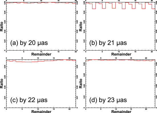
Figure 34. Histogram of intervals for CLEAN component pairs. The horizontal axis shows the remainder of the interval after dividing by d μas. The vertical axis shows the ratio of pairs in a bin. The width of the bin is 1 μas. Panel (a) shows d = 20 μas, (b) d = 21 μas, (c) d = 22 μas, and (d) d = 23 μas.
Download figure:
Standard image High-resolution imageNot only the EHTC image but also our CLEAN image is affected by the sampling bias of the data. As a result, we can see that the structure of the interval d ∼ 43 μas (d = 42.5 ∼44.25 μas) is emphasized.
Such a trend was not observed in our final images. This is probably because the final image is a composite of several CLEAN images (the first two days’ images were created from seven CLEAN images, and the last two days’ images were created from nine CLEAN images.)
Footnotes
- 4
- 5
The M87 black hole mass is still controversial. A mass of
 (68% confidence) is obtained from gas dynamics (Walsh et al. 2013).
 - 6
The EHTC show several different “fiducial” images in their papers. We believe that the images shown in Figure 3 of The Event Horizon Telescope Collaboration et al. (2019a) are the FINAL “fiducial” images of the EHTC because The Event Horizon Telescope Collaboration et al. (2019a) is for reporting the scientific results about “the shadow of the supermassive black hole.”
- 7
The possibility of time variation in brightness temperature cannot be ruled out. The number of measurements is extremely small, and future observations are desirable.
- 8
The referenced EHTC papers do not show the flux density of the ring image.
- 9
First M87 EHT results: calibrated data, https://eventhorizontelescope.org/for-astronomers/data http://datacommons.cyverse.org/browse/iplant/home/shared/commons_repo/curated/theEHTC_FirstM87Results_Apr2019 ~DOI:10.25739/g85n-f134.
- 10
README.md in https://github.com/eventhorizontelescope/2019-D01-01.
- 11
- 12
The sum of the flux densities we obtained with CLEAN components is larger than that of the EHTC ring. We made the ring according to their open procedure and measured its flux density (∼500 mJy).
- 13
The correct image satisfies the closure phase of the observed data. However, the opposite is not always true. Moreover, there are numerous image models that show small closure phase residuals.
- 14
Fringe spacings larger than 100 μas are omitted in the histogram. We are interested in the samplings contributing to very high spatial resolutions less than 100 μas.
- 15
Further, the first sidelobe levels reach more than 70% of the height of the main beam. The sidelobe level is still extremely high even when changing u−v weights. Natural and uniform weighting cases, both show that the first sidelobe levels reach more than 60% of the height of the main beam (see Appendix B).
- 16
- 17
difmap/EHT_Difmap.
- 18
BOXCircMask_r30_x-0.002_y0.022.win on the web.
- 19
Figure 6 in The Event Horizon Telescope Collaboration et al. (2019d) shows similar test results to ours, but they only show the results with BOX sizes narrower than 100 μas in diameter.
- 20
There are 8 plots of “Amplitude versus u−v distance” for M87 in The Event Horizon Telescope Collaboration et al. (2019a, 2019b, 2019c, 2019d, 2019e, 2019f) papers. Figures, where the lower limit of the amplitude axis is 3 mJy, are Figure 2 in The Event Horizon Telescope Collaboration et al. (2019a), Figures 10, 13 in The Event Horizon Telescope Collaboration et al. (2019c), Figure 2 in The Event Horizon Telescope Collaboration et al. (2019d), and Figure 1 in The Event Horizon Telescope Collaboration et al. (2019f). Figure, where the lower limit of the amplitude axis is 5 mJy, is Figure 12 in The Event Horizon Telescope Collaboration et al. (2019d). Figures, where the lower limit of the amplitude axis is 10 mJy, are Figure 13 in The Event Horizon Telescope Collaboration et al. (2019e), and Figure 11 in The Event Horizon Telescope Collaboration et al. (2019f).
- 21
Refer to the NRAO site, http://www.aips.nrao.edu/cgi-bin/ZXHLP2.PL?ROBUST.
- 22
The sidelobe level is extremely high even when changing the u−v weights. Both cases show that the first sidelobe levels reach more than 60% of the height of the main beam.