Abstract
We present 2.5-square-degree C2H N = 1–0 and N2H+ J = 1–0 maps of the ρ Ophiuchi molecular cloud complex. These are the first large-scale maps of the ρ Ophiuchi molecular cloud complex with these two tracers. The C2H emission is spatially more extended than the N2H+ emission. One faint N2H+ clump, Oph-M, and one C2H ring, Oph-RingSW, are identified for the first time. The observed C2H-to-N2H+ abundance ratio ([C2H]/[N2H+]) varies between 5 and 110. We modeled the C2H and N2H+ abundances with 1D chemical models, which show a clear decline of [C2H]/[N2H+] with chemical age. Such an evolutionary trend is little affected by temperatures when they are below 40 K. At high density (nH > 105 cm−3), however, the time it takes for the abundance ratio to drop at least one order of magnitude becomes less than the dynamical time (e.g., turbulence crossing time of ∼105 yr). The observed [C2H]/[N2H+] difference between L1688 and L1689 can be explained by L1688 having chemically younger gas in relatively less dense regions. The observed [C2H]/[N2H+] values are the results of time evolution, accelerated at higher densities. For the relatively low density regions in L1688 where only C2H emission was detected, the gas should be chemically younger.
1. Introduction
With a distance of  (Loinard et al. 2008), the ρ Ophiuchi molecular cloud complex (hereafter ρ-Oph MCC), also called the Ophiuchus Molecular Cloud (e.g., Pattle et al. 2015), is one of the most active star-forming regions within several hundred parsecs of the Sun (Lada & Lada 2003). At such a close distance, the
  beam size (at ∼100 GHz) of a 10 m class millimeter radio telescope corresponds to 0.035 pc. The ρ-Oph MCC consists of Lynds 1688 (hereafter L1688), L1689, and a number of filamentary clouds (L1709, L1740, L1744, L1755, and L1765). These filamentary clouds extending from L1688 are known as the streamers or the cobwebs of the ρ-Oph MCC (Nutter et al. 2006). L1688 is an intermediate-mass star-forming region, filling the gap between low-mass star-forming regions, such as Taurus, and more massive star-forming regions, exemplified by the Orion molecular cloud (Padgett et al. 2008). Motte et al. (1998) identified 13 dense condensations in L1688 from their 1.3 mm dust continuum map with an effective beam resolution of
  (FWHM and all instances hereafter). Johnstone et al. (2004) identified two more objects outside the boundary of previous maps in one 850 μm map with a 40 mJy beam−1 sensitivity and a
  beam size. Stanke et al. (2006) presented a 1.2 mm dust continuum L1688 map with a ∼24″ resolution and a noise level of the order of 10 mJy beam−1. They cleaned their map down to the noise level by using wavelet analysis and identified 143 sources. A possible explanation as to why the number of sources Stanke et al. (2006) identified is much larger than that identified by Motte et al. (1998) is that the condensations in Motte et al. (1998) are split into multiple sources. For example, Oph-B1 was identified as a dense condensation with four starless clumps (B1-MMS1, B1-MMS2, B1-MSS3, and B1-MMS4) in Motte et al. (1998), while at least six sources (MMS20, MMS23, MMS27, MMS28, MMS66, MMS86, and maybe MMS49) were identified by Stanke et al. (2006). Other 1.2 mm dust sources in Stanke et al. (2006) are isolated sources or faint and extended dust emission regions. L1689 is to the east of L1688, associated with less star formation (Loren et al. 1990). To further examine the similarities and differences between L1688 and L1689, we explore here the utility of C2H and N2H+ as tracers.
C2H is a tracer of relatively high density gas with a critical density of  cm−3 (see Appendix
  cm−3 (Appendix
In this paper, we present the first large-scale (2.5-square-degree) C2H N = 1–0 and N2H+ J = 1–0 maps, which cover most high-extinction regions with  in L1688 and L1689, including clumps in earlier studies (e.g., Di Francesco et al. 2004; André et al. 2007).
In Section 2, we present the C2H and N2H+ observations, data reduction, and the Infrared Astronomy Satellite (IRAS) dust temperature map. The calculation of the C2H-to-N2H+ abundance ratio ([C2H]/[N2H+]) is presented in Section 3. Our chemical model and interpretation are given in Section 4. Comparative studies of C2H and N2H+ in terms of centroid velocity, line width, and [C2H]/[N2H+] are in Section 5. Conclusions are presented in Section 6. Details of critical density estimation and column density calculation are given in the appendices.
2. Observation and Data Reduction
2.1. The C2H and N2H+ Data
The ρ-Oph MCC was mapped with the Delingha 13.7 m telescope of Qinghai Station,7 Purple Mountain Observatory (PMO), Chinese Academy of Sciences. The observations were carried out in position switching mode in 2012 December and 2013 January, March, and April.
At Delingha, the ρ-Oph MCC stays above 20° elevation with a maximum of 28° for approximately 5 hr per day. To obtain low system temperatures, we only took data for 2 hr around maximum source elevation.
The 3 × 3 Superconductor-Insulator-Superconductor receiver array of the Delingha telescope (Shan et al. 2012; Zuo et al. 2011) can observe 85–115 GHz. The backend consists of 18 fast Fourier transform spectrometers, each with 16,384 channels. The backend operates in two modes, a 200 MHz bandwidth with 12.2 kHz channel width and a 1000 MHz bandwidth with 61.0 kHz channel width.
As a first test observation, we performed on the fly (OTF) mapping of the Oph-A region with a 200 MHz bandwidth (Δv ∼ 0.05 km s−1) to see whether the velocity resolution in the 1000 MHz bandwidth (Δv ∼ 0.20 km s−1) is suitable for fitting the centroid velocity and line width. The test observation covered a 15′ × 15′ square region centered on the position of Oph-A with the highest Two Micron All Sky Survey (2MASS) extinction. Hyperfine structure fitting was done. The data were then smoothed to a 0.20 km s−1 velocity resolution before another round of fitting was performed. A comparison between these two fitting results showed that the hyperfine structure fitting of spectra with strong emission is affected little by this smoothing, and thus the 0.20 km s−1 velocity resolution is sufficient for observing N2H+ in the ρ-Oph MCC and analysis using hyperfine fitting. For example, the original spectrum with a ∼4 K  peak at the position 16h26m26
5, −24°24′09″ (J2000) showed a centroid velocity of 3.60 ± 0.01 km s−1, a line width of 0.60 ± 0.03 km s−1, an optical depth of 0.73 ± 0.2, and an excitation temperature of
 K from hyperfine fitting. After smoothing to 0.2 km s−1, the centroid velocity was 3.60 ± 0.01 km s−1, the line width was 0.60 ± 0.03 km s−1, the optical depth was 0.73 ± 0.25, and the excitation temperature was
  K. In this example, only the uncertainties became slightly larger. Compared with the crowded N2H+ hyperfine structures, the C2H spectra have six well-separated hyperfine components. Observing these six components requires a much lower velocity resolution in a wider bandwidth. The 1000 MHz mode provides enough velocity resolution for C2H hyperfine structure fitting. For spectra with weak emission, however, we performed hyperfine fitting and found that the results were affected by the smoothing. In the following, we only applied the resulting opacity correction to N2H+ spectra with an integrated intensity of 3 K km s−1 or higher and to C2H spectra above 2 K km s−1. Low opacities were assumed for spectra with weak emission.
The COordinated Molecular Probe Line Extinction Thermal Emission Survey of Star-forming Regions (Ridge et al. 2006, hereafter COMPLETE) provides the 2MASS NICER extinction map and IRAS dust temperature map of the ρ-Oph MCC. These maps were used for observation region selection. In L1688, six 30′ × 30′ areas were selected, covering most regions with extinction  . L1689 was covered by four
  areas next to the observation region of L1688. Reference positions were chosen from the COMPLETE ρ-Oph MCC 12CO and 13CO maps. Tables 1 and 2 show the details of observation.
Table 1. Observation Information of 10 30′ × 30′ OTF Scans
| No. | Center R.A. | Center Decl. | Ref. Position | Ref. Position | Scan Rate | Sample Interval | Scan Time | Total Scan Time |
|---|---|---|---|---|---|---|---|---|
| (J2000) | (J2000) | R.A. (J2000) | Decl. (J2000) | (arcsec s−1) | (s) | (minutes) | (minutes × repeats) | |
| 01 | 16h26m16s | −24°20′54″ | 16h29m29s | −24°29′31″ | 50 | 0.3 | 85 | 85 × 4 |
| 02 | 16h28m16s | −24°20′54″ | 16h30m32s | −24°07′28″ | 50 | 0.3 | 85 | 85 × 4 |
| 03 | 16h24m16s | −24°20′54″ | 16h26m18s | −23°46′10″ | 50 | 0.3 | 85 | 85 × 4 |
| 04 | 16h26m16s | −24°50′54″ | 16h30m32s | −24°07′28″ | 50 | 0.3 | 85 | 85 × 4 |
| 05 | 16h28m16s | −24°50′54″ | 16h30m32s | −24°07′28″ | 75 | 0.2 | 45 | 60 × 6 |
| 06 | 16h24m16s | −24°50′54″ | 16h26m18s | −23°46′10″ | 75 | 0.2 | 45 | 60 × 6 |
| 07 | 16h30m16s | −24°30′00″ | 16h30m16s | −24°18′00″ | 75 | 0.2 | 45 | 60 × 6 |
| 08 | 16h32m16s | −24°30′00″ | 16h32m16s | −24°18′00″ | 75 | 0.2 | 45 | 60 × 6 |
| 09 | 16h30m16s | −25°00′00″ | 16h30m16s | −24°18′00″ | 75 | 0.2 | 45 | 60 × 6 |
| 10 | 16h32m16s | −25°00′00″ | 16h32m16s | −24°18′00″ | 75 | 0.2 | 45 | 60 × 6 |
Download table as: ASCIITypeset image
Table 2. Frequency Settings of the Observation
| Lines | Rest Frequency | Relative Intensity |
|---|---|---|
| (MHz) | ||
C2H N = 1–0 J =  – – F = 1–1 F = 1–1 |
87284.38 | 4.25 |
C2H N = 1–0 J =  – – F = 2–1 F = 2–1 |
87317.05 | 41.67 |
C2H N = 1–0 J =  – – F = 1–0 F = 1–0 |
87328.70 | 20.75 |
C2H N = 1–0 J =  – – F = 1–1 F = 1–1 |
87402.10 | 20.75 |
C2H N = 1–0 J =  – – F = 0–1 F = 0–1 |
87407.23 | 8.33 |
C2H N = 1–0 J =  – – F = 1–0 F = 1–0 |
87446.42 | 4.25 |
| N2H+ J = 1–0 F1 = 1–1 F = 0–1 | 93171.6086 | 0.33334 |
| N2H+ J = 1–0 F1 = 1–1 F = 2–1 | 93171.9054 | 1.66667 |
| N2H+ J = 1–0 F1 = 1–1 F = 1–1 | 93172.0403 | 1.00000 |
| N2H+ J = 1–0 F1 = 2–1 F = 2–1 | 93173.4675 | 1.66667 |
| N2H+ J = 1–0 F1 = 2–1 F = 3–1 | 93173.7643 | 2.33333 |
| N2H+ J = 1–0 F1 = 2–1 F = 1–1 | 93173.9546 | 1.00000 |
| N2H+ J = 1–0 F1 = 0–1 F = 1–1 | 93176.2527 | 1.00000 |
Note. The frequencies and relative intensities of C2H are from Tucker et al. (1974); the frequencies and relative intensities of N2H+ are from Keto & Rybicki (2010). C2H is in the lower sideband, and N2H+ is in the upper sideband.
Download table as: ASCIITypeset image
The original OTF data were regridded with a pixel size of  . In the regridding procedure, spectra with extremely bad baselines or high rms values were removed, since these spectra may be caused by hardware errors. A 60% main-beam efficiency was used in the calibration. The data were uploaded to the Millimeter Wave Radio Astronomy Database.8
,9
,10
The astronomical software package Gildas/CLASS11
was used for further reduction.
. In the regridding procedure, spectra with extremely bad baselines or high rms values were removed, since these spectra may be caused by hardware errors. A 60% main-beam efficiency was used in the calibration. The data were uploaded to the Millimeter Wave Radio Astronomy Database.8
,9
,10
The astronomical software package Gildas/CLASS11
was used for further reduction.
Given the relatively low elevation of the observations, the spectral baselines are complex. A fifth-order polynomial was subtracted from each C2H spectrum. For N2H+ data, a third-order polynomial was used. The OTF data were combined into one file for regridding. In regridding, the velocity resolutions are 0.21 km s−1 for C2H spectra and 0.20 km s−1 for N2H+ spectra. After regridding, only spectra with rms values less than 0.5 K ( ) were selected. For C2H spectra, velocity ranges of [−50, −40], [−30, 0], and [10, 50] km s−1 were used for rms calculation. For N2H+ spectra, the velocity ranges used were [−50, −8] and [15, 50] km s−1. Though the rms values of the spectra near map edges were still less than 0.5 K (
 ), the baselines of these spectra were too complex for polynomial fitting. Hence, spectra near map edges were rejected.
The integrated intensity maps of C2H and N2H+ are shown in Figure 1. For C2H, to present a uniform integrated intensity map, we selected two strongest hyperfine components that were widely detected. The selected velocity ranges for these two components in spectra were [−39.1, −35.1] and12 [1.9, 5.0] km s−1. When calculating the N2H+ integrated intensity, we selected three hyperfine components, corresponding to a velocity range of13 [2.0, 6.0] km s−1. The rms values of C2H and N2H+ integrated intensity maps are 0.8 and 0.4 K km s−1, respectively. A 5 × 5 pixel boxcar smoothing was then performed to the integrated intensity maps for drawing contours.
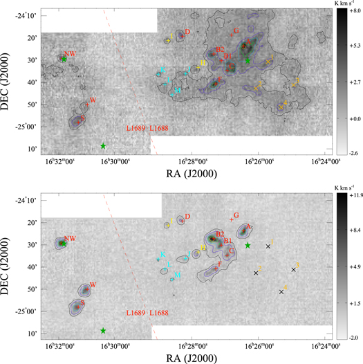
Figure 1. C2H integrated intensity map (top) and N2H+ integrated intensity map (bottom). The data are smoothed with a boxcar average of a 5 × 5 pixel box only for drawing contours. In the C2H map, black, purple, blue, green, and yellow contours show the smoothed C2H integrated intensities at levels of 1, 2, 3, 4, and 5 K km s−1, respectively. In the N2H+ map, black, purple, blue, green, and yellow contours show the integrated intensities at levels of 0.8, 1.6, 3.2, 4.8, and 6.4 K km s−1, respectively. Red and yellow plus signs with labels show the dust clumps in L1688 (red: Motte et al. 1998; yellow: Johnstone et al. 2004) and L1689 (red: Nutter et al. 2006). Orange crosses with labels show four selected positions with C2H emission peaks in the molecular ring Oph-RingSW. In the N2H+ integrated intensity map, to see these symbols clearly with a gray background, crosses are in black. Light-blue plus signs with labels show our four newly named N2H+ clumps. Three dark green stars show the position of the protostar I16293 (left, 16h32m22753 −24°28′34
747, J2000, in Kristensen et al. 2013), the star 22 Scorpius (bottom, 16h31m06
24 −25°08′40
7, J2000), and the star HD 147889 (right, 16h26m17
74 −24°29′47
9, J2000). In L1688, red, yellow, and light-blue letters A through M stand for sources Oph-A through M, and orange numbers 1 through 4 stand for sources L1688-C2H-1 through 4. In L1689, three red labels from north to south stand for L1689NW, L1689W, and L1689S. In Section 3.1, the four N2H+ clumps with light-blue plus signs and labels are discussed. In Section 5.1, the C2H and N2H+ spectra in the 14 positions with red plus signs (except G), orange crosses, or yellow plus signs (H only) are discussed.
Download figure:
Standard image High-resolution imageThe weather and the relatively low elevation are the main reasons for the variation of rms values. When the observation region is close to its maximum elevation and the weather is good, a typical system temperature is between 160 and 170 K, which increases to 200 K or higher under bad weather or low elevation. The variation of the system temperature caused an approximately ±0.1 K km s−1 variation of the rms values of the smoothed C2H and N2H+ spectra in different regions. The actual sky coverage of each 30′ × 30′ OTF map is a little larger. Around the edges with overlapped scans, we averaged both data sets to lower the rms values.
2.2. IRAS Temperature Map from COMPLETE
We downloaded the IRAS dust temperature map of the ρ-Oph MCC from the COMPLETE project Web page.14 The IRAS dust temperature map was derived from infrared images in the latest release of the IRAS data set (IRIS15 ). The description of the method used to derive the IRAS dust temperature can be found in Schnee et al. (2005). The IRAS dust temperature map of the whole ρ-Oph MCC region was published by Ridge et al. (2006).
The sky coverage and pixel size of the IRAS dust temperature map differ from those of our C2H and N2H+ spectral data cubes. An IDL code, hastrom in the NASA IDL Astronomy User’s Library,16 was used to crop and resample the temperature maps so that the sky coverage and pixel size of the processed map match those of our C2H and N2H+ integrated intensity maps. The IRAS dust temperatures were used as proxies of the excitation temperatures.
3. Results
3.1. Integrated Intensity Maps of C2H and N2H+
In L1688, eight 1.3 mm dust clumps (Oph-A through G, Motte et al. 1998, red plus signs with labels in Figure 1) and two 850 μm dust clumps (Oph-H and Oph-I, Johnstone et al. 2004, yellow plus signs with labels in Figure 1) were all detected in N2H+ emission within one ∼60″ beam. There is an extremely faint N2H+ clump toward the position of Oph-G with an averaged N2H+ integrated intensity of 0.8 K km s−1 in a 3 × 3 pixel region. After being smoothed by a 5 × 5 pixel box, the integrated intensity here becomes lower than 0.8 K km s−1, and thus no contours are seen there in Figure 1. Four more faint N2H+ clumps in L1688 have been identified, namely, Oph-J (the N2H+ peak at 16h28m24s, −24°36′12″, J2000), Oph-K (the N2H+ peak at 16h29m17s, −24°36′05″, J2000), Oph-L (the N2H+ peak at 16h29m03s, −24°40′45″, J2000), and Oph-M (the N2H+ peak at 16h28m47s −24°45′04″, J2000). Oph-J is the brightest among these four clumps, with a 1.6 K km s−1 peak N2H+ integrated intensity (4.2σ). It was previously detected via 1.1 mm dust continuum (Bolo 26 in Young et al. 2006) and separated into four cores in the 1.2 mm dust continuum, namely, MMS-60, 126, 130, and 99 in Stanke et al. (2006). Oph-L is the next brightest clump, with a 1.2 K km s−1 peak N2H+ integrated intensity (3.2σ). At least three 1.2 mm dust cores (MMS-92, 109, and 122; Stanke et al. 2006) are embedded in Oph-L, Oph-K, and Oph-M, each of which has 0.9 K km s−1 peak N2H+ integrated intensity (2.3σ). Oph-K was previously detected via 1.2 mm dust continuum, and two cores were identified as MMS-102 and MMS-119 by Stanke et al. (2006). Without previously known dust peaks, Oph-M is identified for the first time in this data set.
We also identified a C2H molecular ring, Oph-RingSW, in the relatively diffuse region southwest of L1688. Some parts of this ring can also be found in the COMPLETE 12CO map of L1688. The origin of this ring is unknown.
In Section 5.2, we select the C2H and N2H+ spectra at various peaks, perform the hyperfine fittings, compare the centroid velocities and line widths, and check whether the N2H+ emission peak and the dust emission peak of the clumps Oph-A through F and H are located within one beam (60″).
3.2. Column Densities and C2H-to-N2H+ Ratios
Some positions in L1688 and L1689 have weak C2H or N2H+ emission. The integrated intensities at these positions are significant, but the spectra themselves are too weak for hyperfine fitting, e.g., the C2H spectrum in L1689NW (see Table 3). We assumed optically thin emission and followed the recipe below (see, e.g., Li 2002).
Table 3. Mean Chemical Ages
| Density NH | L1688 Mean Age | L1689 Mean Age |
|---|---|---|
| (cm−3) | (yr) | (yr) |

|

|

|

|

|

|

|

|

|

|

|

|
Download table as: ASCIITypeset image
The column density of an upper-level population of an optically thin transition is

where  is the integrated intensity consisting of all six hyperfine components of the C2H spectra or all seven hyperfine components of the N2H+ spectra. In addition, k is the Boltzmann constant, h is the Planck constant, ν is the frequency, and c is the speed of light. The total column density is

where Fu,  , and Fb are the level correction factor, the opacity correction factor, and the correction factor for the background, respectively. In this calculation, we only calculated the C2H column densities at positions with a C2H integrated intensity of 1.5 K km s−1 or higher. The threshold for N2H+ column density calculation was 2 K km s−1. The details can be found in Appendix
We applied the opacity correction to N2H+ spectra with integrated intensities over [−8, 15] km s−1 greater than 3.0 K km s−1 and optical depths between 0.5 and 5.0. If the fitted optical depth was below 0.5 or above 5.0, however, noise may have made the result unreliable by skewing the peak temperature ratios between hyperfine components, depending on the signal-to-noise ratios of the components. Ignoring an optical depth of 0.5 will lead to an underestimation of 27%. A similar opacity correction was also done for C2H spectra but for the spectra with integrated intensity greater than 1.0 K km s−1.
In our C2H and N2H+ column density calculations, using IRAS dust temperatures as excitation temperatures of C2H and N2H+ can cause large uncertainty. For example, the original IRAS temperatures have an  pixel size and a 4
3 spatial resolution (Schnee et al. 2005). This spatial resolution is approximately four times lower than our molecular line data. The IRAS temperatures come from far-infrared fluxes and may overestimate temperatures in compact, dense cores. Using the Herschel Space Observatory 160 and 250 μm dust continuum maps and James Clerk Maxwell Telescope 450 and 850 μm dust continuum maps, Pattle et al. (2015) derived the mean line-of-sight dust temperatures of sources in the ρ-Oph MCC by fitting the spectral energy distribution with a modified blackbody distribution. These temperatures are lower than the IRAS temperatures. Lower temperatures result in lower C2H and N2H+ column densities. For example, in the location of the source SM1 (see Motte et al. 1998; 16h26m27
36, −24°23′52
8, J2000), the C2H and N2H+ integrated intensities are 12.3 and 12.0 K km s−1, respectively. Using the IRAS temperature (37 K), the column densities of C2H and N2H+ are 6.8 × 1013 cm−2 and 3.1 × 1012 cm−2, respectively. These two column densities are both 4.6 times higher than those estimated with the temperature (17.2 ± 0.6 K) in the same location in Pattle et al. (2015).
The ratio between the column densities, however, is impervious to the temperature uncertainty for cloud conditions relevant here. We therefore use [C2H]/[N2H+] to explore the chemical evolution and physical properties of ρ-Oph MCC. [C2H]/[N2H+] represents both the column density ratio of C2H and N2H+ and the abundance ratio of C2H and N2H+. Figure 2 shows an example of [C2H]/[N2H+] changing with different temperatures when the integrated intensities of C2H or N2H+ are all assumed to be 5 K km s−1. The [C2H]/[N2H+] values under different temperatures in Figure 2 come from the column density and abundance ratio calculations that are mentioned above and in Appendix
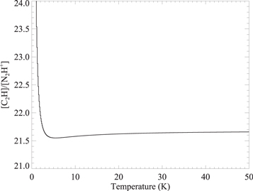
Figure 2. An example to show that [C2H]/[N2H+] values are less affected by different temperatures. For the given C2H and N2H+ integrated intensities (both are 5 K km s−1 here), the values of [C2H]/[N2H+] change little when the temperature is between ∼7 and 50 K.
Download figure:
Standard image High-resolution imageFigure 3 shows the distribution of the measured abundance ratio in L1688 and L1689, which varies between 5 and 110. The differences in the distribution of the abundance ratio will be mentioned in Section 5.
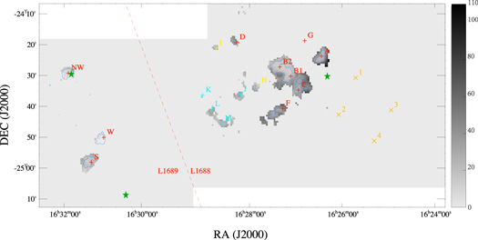
Figure 3. Distribution of [C2H]/[N2H+]. Blue contours represent the regions with 5 K km s−1 or higher N2H+ integrated intensities. Symbols and labels are the same as those in Figure 1.
Download figure:
Standard image High-resolution image4. Chemical Model
To interpret our data, we modeled [C2H]/[N2H+] evolution with both the pure gas and gas-grain chemical networks.
The simulation was performed using Nautilus, a gas-grain chemical code (Hersant et al. 2009), along with the gas-grain chemical reaction network from Hincelin et al. (2011, 2013). An electronic version of the network is available in the KInetic Database for Astrochemistry database17
(Wakelam et al. 2012). Low metal abundances, as in Semenov et al. (2010), had been assumed for the initial gas phase abundances. Initially, all species were in the gas phase. The cosmic-ray ionization rate was set to  s−1. The size of dust grains was assumed to be the same, with a radius of 0.1 μm. Both pure gas phase and gas-grain network simulations were carried out for comparative studies. Four different temperatures (10, 20, 30, and 40 K) and four different densities (5 × 10³, 2 × 10⁴, 1 × 10⁵, and 1 × 106 cm−3) were applied in our simulations.
Our simulations are purely chemistry models without dynamic evolution. This is sufficient for examining the cloud chemistry as long as the timescale for density variation is much longer than the chemical relaxation time, which is a reasonable assumption for the densities concerned here.
We compared the pure gas model and the gas-grain model. Figure 4 shows the C2H abundance, N2H+ abundance, and [C2H]/[N2H+] as functions of time in a pure gas phase model and a gas-grain model with  cm−3 and
  cm−3, respectively. The temperature in both models is fixed at 10 K. The most pronounced difference between these two models shows up in the abundance of C2H. It remains constant or rises slightly in gas-grain models, whereas in pure gas models, it plummets after approximately 105–106 yr. The major destruction route of C2H is reaction with O to form CO, while its major production route is the dissociative recombination of C2H
 and C2H
 . Since only neutral species are allowed to accrete on grain surfaces in our gas-grain reaction network simulation, the abundances of C2H
 and C2H
 in the gas-grain model are not all that different from those in the pure gas model. O can be frozen on grain surfaces as H2O and be largely depleted from the gas phase in later stages of the gas-grain model. C2H experiences a lower destruction rate in gas-grain networks. Thus, the C2H abundance in late stages is sensitive to the existence of dust, mainly due to depletion of O onto grain surfaces. For N2H+, its major production route is the reaction

while its major destruction route is reaction with CO (e.g., Turner 1995; Vasyunina et al. 2012). The depletion temperatures of both N2 and CO are similar and lower than 20 K. Such temperatures lead to the result that the trend of the change of N2H+ abundance is little affected by adding the dust into the model. Thus, the N2H+ abundance keeps rising in both the pure gas and gas-grain models, until t ∼ 106 yr. After t ∼ 106 yr, the decreasing of N2H+ abundance is the result of the evolution of CO, N2, and  . Comparing the models with and without dust, the [C2H]/[N2H+] values are insensitive to the existence of dust, also until t ∼ 106 yr. We use the gas-grain model in subsequent analyses. It is also worth noting that there is no significant difference seen in the evolution of C2H abundances or N2H+ abundances between two densities that differ by a factor of 5.
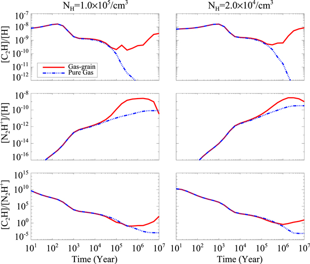
Figure 4. Results of pure gas and gas-grain models at a fixed temperature of 10 K. The red solid line shows the gas-grain model calculation of the C2H abundance, the N2H+ abundance, and the [C2H]/[N2H+]. The blue dot-dashed line shows the results of the pure gas model.
Download figure:
Standard image High-resolution imageWe ran the model with different extinctions and UV field strengths to see whether the variations of these two parameters affect the chemical evolution. In the model, both the extinction and the UV field affect the photodissociation rate coefficients (PRCs), which are proportional to  . The factor γ is a value around 2, depending on the balance between molecular photon absorption and differential dust absorption, AV is the extinction, G0 = 1.6 × 10⁻³ erg s−1 cm−2 is the unit of UV field, and F0 is the scaling factor of the UV field. We ran the chemical model with two sets of parameter grids: (1) F0 = 1, density
  cm−3, temperature T = 30 K, and extinctions AV = 1, 5, 8, and 20 mag; and (2) F0 = 0.01, 100, 1000, and 10,000, density
  cm−3, temperature T = 30 K, and extinction AV = 10 mag.
Different parts of molecular clouds may be exposed to different external far-UV (FUV) radiation fields, and different positions in molecular clouds have different extinctions. These variations produce different chemical products in different parts of a molecular cloud. The PRCs for cosmic-ray-induced secondary photons, however, are independent of AV. For visual extinction AV = 10 mag, the PRCs due to secondary photons are more than three orders of magnitude larger than those of the external FUV radiation in our reaction network (Hincelin et al. 2011, 2013). Thus, the variation of AV and the scaling factor do not affect the chemical evolution much in our models if AV is larger than 10 mag. In our map, the extinction values in the place with C2H or N2H+ emissions are relatively high (e.g., 10 mag). We expect that the variation of extinction and external FUV radiation fields has little effect on the chemical evolution of dense molecular clouds.
The extinctions at almost all the positions of the N2H+ clumps fulfill AV ≥ 10 mag. Figure 5 shows the evolutionary trends of the abundances of C2H or N2H+ and their abundance ratio under different extinctions. We see that the C2H abundance, the N2H+ abundance, and the [C2H]/[N2H+] all hardly differ for AV ≥ 8 mag, and the C2H abundance is more easily affected by the different extinctions. The evolution of [C2H]/[N2H+] with time differs substantially when AV = 1 mag. Therefore, we ignored differences in extinctions and used 10 mag as the basis for further model simulations.
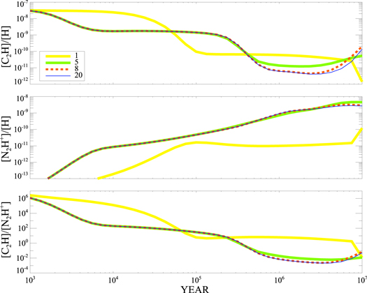
Figure 5. Gas-grain model calculation of C2H abundance evolution of N2H+ and [C2H]/[N2H+] under different extinctions. The yellow solid line, green solid line, red dashed line, and blue solid line show the results for extinctions AV = 1, 5, 8, and 20 mag, respectively. F0 = 1 was used for all cases.
Download figure:
Standard image High-resolution imageFigure 6 shows the evolutionary trends of the abundances of C2H or N2H+ and the abundance ratio under different external UV fields. With extinction 10 mag, four models with F0 values of 0.01, 100, 1000, and 10,000 are shown. From the early evolutionary time of 103 yr to ∼5 × 10⁵ yr for C2H or from 103 yr to ∼2 × 10⁶ yr for N2H+, the model calculation results were little affected by the different F0 values from 0.01 to 10,000. From the later evolutionary time of ∼5 × 10⁵ yr to 107 yr for C2H or from ∼2 × 10⁶ yr to 107 yr for N2H+, the C2H and N2H+ abundances only slightly increase by factors of ∼10 and 5, respectively. As seen from Figure 5, when extinctions are high enough, both C2H and N2H+ abundances are barely affected by the external UV field. For a cloud with extinction AV = 10 mag, however, the chemical evolution will be affected by the external UV field when F0 reaches 1000. Liseau et al. (1999) estimated the UV field in the ρ-Oph MCC by sampling 33 positions, including Oph-A, Oph-B1, Oph-B2, Oph-C1, and Oph-D. The F0 values (F in Liseau et al. 1999) in these 33 positions are all below 150. Therefore, we ignored the differences in external UV field and used F0 = 1 for further simulations.
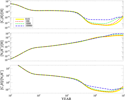
Figure 6. Gas-grain model calculation of C2H abundance, N2H+ abundance, and [C2H]/[N2H+] with different values of F0. The yellow solid line, red dashed line, green dot-dashed line, and blue dashed line show the results of F0 of 0.01, 100, 1000, and 10,000, respectively. AV = 10 mag was used for all cases.
Download figure:
Standard image High-resolution imageFigure 7 shows the abundances of C2H and N2H+ and [C2H]/[N2H+] as functions of time for different temperatures and densities in the gas-grain model. Here, we find that the C2H abundance depends strongly on temperature and density. These dependencies can be explained from the formation and destruction routes of C2H. The abundance of  plays a crucial role in the production of C2H. Protonated methane is produced by radiative association of C+ with H2 and hydration addition reactions. All carbon atoms are in the form of
  in the beginning of the model and are gradually converted to species such as CO or protonated methane. Thus, the abundance of C2H increases in the beginning when abundances of methane or species such as CO and OH also increase. Atomic O accretes on grain surfaces and reacts with other species, and thus is depleted from the gas phase. At 10 K, when most gas phase O atoms are depleted after approximately 2 × 10⁶ yr, C2H can hardly be destroyed and the abundance of C2H increases again. Indeed, our simulation results bear out this trend. O starts to desorb from grain surfaces at around 15 K. As temperature increases, it becomes increasingly difficult to freeze atomic O on grain surfaces. Hence, C2H abundance decreases with increasing temperature at late stages. Density also affects C2H abundance. The dependence of C2H abundance on density is due to both O and C+ depleting more quickly from the gas phase when density increases. The desorption of O at around 15 K is also the reason that the 20 K models differ so dramatically from those at lower and higher temperatures.
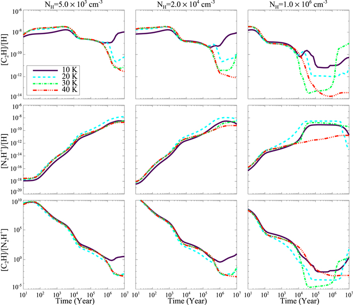
Figure 7. Gas-grain model calculation of C2H abundance, N2H+ abundance, and [C2H]/[N2H+]. Each column shows the result for the same density. The densities are shown as the titles of the first plots of the column. The dark-purple solid line, light-blue dashed line, light-green dot-dashed line, and red dot-dashed line show the calculation of the gas-grain model with 10, 20, 30, and 40 K, respectively.
Download figure:
Standard image High-resolution imageThe situation is different for the changes of N2H+ abundances. The major production and destruction routes of N2H+ are related to N2 and CO, respectively. The desorption energies are 1000 K for N2 and 1150 K for CO. Both N2 and CO can be depleted from the gas phase when the temperature is lower than 20 K. The relative abundance of these two species determines the abundance of N2H+. The N2H+ abundance is affected little by temperature and volume density variations.
Combining the evolutions of both species, the [C2H]/[N2H+] decreases with time between 102 and 106 yr for a volume density of 5.0 × 103 cm−3 and from the beginning to approximately 2.0 × 10⁴ yr for a volume density of 1.0 × 106 cm−3. This evolutionary trend is little affected by temperature for Tk < 40 K. At high density (nH > 105 cm−3), the time it takes for the abundance ratio to drop at least one order of magnitude becomes less than the typical dynamical time. For example, a 0.1 pc clump at the distance of ρ-Oph MCC spans about 29, implying a turbulence crossing time of ∼105 yr for a characteristic 1 km s−1 turbulence velocity.
Concerning the observed [C2H]/[N2H+] values, the trends for all three modeled densities are consistently decreasing with time. The possible volume densities in the positions with the observed [C2H]/[N2H+] values are 1.0 × 105 cm−3 or higher (see, e.g., Motte et al. 1998; Young et al. 2006). In such conditions, the [C2H]/[N2H+] values are more sensitive to the volume densities than to the chemical ages, as we describe below.
5. Discussion
5.1. [C H]/[NH as a Tracer of Chemical Evolution and Volume Density


![${}^{+}]$](https://content.cld.iop.org/journals/0004-637X/836/2/194/revision1/apjaa5c33ieqn59.gif)
According to our chemical model, the C2H abundance decreases while the N2H+ abundance increases with time (see Figure 7). Therefore, [C H]/[N
H]/[N H
H![${}^{+}]$](https://content.cld.iop.org/journals/0004-637X/836/2/194/revision1/apjaa5c33ieqn62.gif) can be used as a tracer of chemical evolution. Figure 8 shows a comparison between the observed [C
can be used as a tracer of chemical evolution. Figure 8 shows a comparison between the observed [C H]/[N
H]/[N H
H![${}^{+}]$](https://content.cld.iop.org/journals/0004-637X/836/2/194/revision1/apjaa5c33ieqn65.gif) values in L1688 or L1689 and models of different volume density and temperature. The mean estimated chemical ages of the observed [C
values in L1688 or L1689 and models of different volume density and temperature. The mean estimated chemical ages of the observed [C H]/[N
H]/[N H
H![${}^{+}]$](https://content.cld.iop.org/journals/0004-637X/836/2/194/revision1/apjaa5c33ieqn68.gif) values in L1688 (yellow squares in Figure 8) or L1689 (purple triangles in Figure 8) are listed in Table 3. Linear interpolation is used to include our observed [C
values in L1688 (yellow squares in Figure 8) or L1689 (purple triangles in Figure 8) are listed in Table 3. Linear interpolation is used to include our observed [C H]/[N
H]/[N H
H![${}^{+}]$](https://content.cld.iop.org/journals/0004-637X/836/2/194/revision1/apjaa5c33ieqn71.gif) values with the modeled data. The details of the interpolation can be found in Appendix
values with the modeled data. The details of the interpolation can be found in Appendix
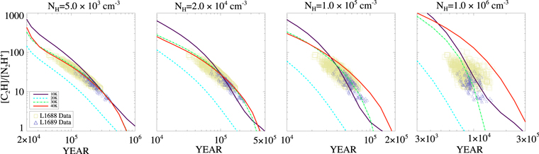
Figure 8. Modeled [C2H]/[N2H+] (lines) as a function of evolutionary time with the real observation data (squares and triangles). In each plot, the dark-purple solid line, light-blue dashed line, light-green dot-dashed line, and red dot-dashed line show the calculation results of the gas-grain model with temperatures of 10, 20, 30, and 40 K, respectively. Squares and triangles show observed [C2H]/[N2H+] values of each pixel in L1688 and L1689, respectively. In this figure, the modeled data we use are the same as those in Figure 7. To show the observed data points clearly, we use the different scales on both axes.
Download figure:
Standard image High-resolution imageFigure 8 shows that both chemical ages and volume densities affect the [C H]/[N
H]/[N H
H![${}^{+}]$](https://content.cld.iop.org/journals/0004-637X/836/2/194/revision1/apjaa5c33ieqn74.gif) values. In the first and second panels from the left of Figure 8, the chemical ages of the observed [C
values. In the first and second panels from the left of Figure 8, the chemical ages of the observed [C H]/[N
H]/[N H
H![${}^{+}]$](https://content.cld.iop.org/journals/0004-637X/836/2/194/revision1/apjaa5c33ieqn77.gif) are both around 105 yr. In such a volume density range, the estimated chemical ages seem to be affected more by the [C2H]/[N2H+] values than by different volume densities. From left to right, in the third and fourth panels in Figure 8, for these same observed [C
are both around 105 yr. In such a volume density range, the estimated chemical ages seem to be affected more by the [C2H]/[N2H+] values than by different volume densities. From left to right, in the third and fourth panels in Figure 8, for these same observed [C H]/[N
H]/[N H
H![${}^{+}]$](https://content.cld.iop.org/journals/0004-637X/836/2/194/revision1/apjaa5c33ieqn80.gif) values, the estimated ages decrease to ∼5 × 10⁴ yr and ∼1 × 10⁴ yr, respectively. For the same [C
values, the estimated ages decrease to ∼5 × 10⁴ yr and ∼1 × 10⁴ yr, respectively. For the same [C H]/[N
H]/[N H
H![${}^{+}]$](https://content.cld.iop.org/journals/0004-637X/836/2/194/revision1/apjaa5c33ieqn83.gif) values and in high volume density gas, Figure 8 shows that higher volume densities result in younger estimated ages of the same observed abundance ratios, and both the [C2H]/[N2H+] values and volume densities affect the chemical ages at similar levels. In addition, the relationship between the time/chemical age and [C2H]/[N2H+] steepens when the volume density increases. The mean ages in Table 3 corresponding to the observed [C
values and in high volume density gas, Figure 8 shows that higher volume densities result in younger estimated ages of the same observed abundance ratios, and both the [C2H]/[N2H+] values and volume densities affect the chemical ages at similar levels. In addition, the relationship between the time/chemical age and [C2H]/[N2H+] steepens when the volume density increases. The mean ages in Table 3 corresponding to the observed [C H]/[N
H]/[N H
H![${}^{+}]$](https://content.cld.iop.org/journals/0004-637X/836/2/194/revision1/apjaa5c33ieqn86.gif) values in L1688 or L1689 decrease more when the volume density increases to higher volume density ranges. For example, when the volume density increases 20 times from 5.0 × 103 cm−3 to 1 × 105 cm−3, the derived chemical mean age corresponding to the observed abundance values in L1688 decreases from 1.4 × 10⁵ yr to one-third of this value. When the volume density increases 10 times further from 105 cm−3, the derived chemical mean age corresponding to the observed abundance values in L1688 decreases from 4.4 × 10⁴ yr to one-fifth of that value.
values in L1688 or L1689 decrease more when the volume density increases to higher volume density ranges. For example, when the volume density increases 20 times from 5.0 × 103 cm−3 to 1 × 105 cm−3, the derived chemical mean age corresponding to the observed abundance values in L1688 decreases from 1.4 × 10⁵ yr to one-third of this value. When the volume density increases 10 times further from 105 cm−3, the derived chemical mean age corresponding to the observed abundance values in L1688 decreases from 4.4 × 10⁴ yr to one-fifth of that value.
Figure 9 in another way shows the relationship between [C2H]/[N2H+], the chemical age, and the volume density. The top panel shows, using models, how [C2H]/[N2H+] is affected by chemical age. When the volume density is low, e.g., 5 × 103 cm−3, the abundance ratios at different ages look distinct in the panel. When volume density is high, e.g., 106 cm−3, the abundance ratios at different ages seem to be indistinct in the panel. Note that the axis for chemical age (Y-axis) is linear to reflect the chemical age decreasing when the volume density is increasing; thus, the total range variation at high density is hard to recognize in such a panel, although they may still be significant. The bottom panel shows how [C2H]/[N2H+] is affected by volume density. When the volume density is 105 cm−3 or lower, chemical age changes of one order of magnitude higher or lower result in [C2H]/[N2H+] changes of only ∼1.5 orders of magnitude lower or higher, respectively. When the volume density is 106 cm−3, however, [C2H]/[N2H+] drops roughly seven orders of magnitude lower when the chemical age only increases one order of magnitude higher. It appears that 105 cm−3 is roughly the critical value between the regimes where [C2H]/[N2H+] is sensitive to volume density or not.
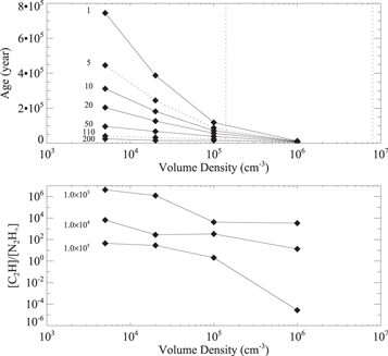
Figure 9. Modeled [C2H]/[N2H+] values vary with chemical ages (upper) or different volume densities (lower) when Tk = 30 K. In the top panel, the solid lines and nonvertical dotted lines show how the estimated ages change with one [C2H]/[N2H+], of which the value is shown at the left of the line. The two nonvertical dotted lines show the minimum and maximum values of the observed [C2H]/[N2H+] values. The two vertical dotted lines show the positions with volume densities of 1.4 × 105 cm−3 to 8.0 × 106 cm−3, respectively. In the bottom panel, each line shows how the [C2H]/[N2H+] values change with one chemical age, of which the value is shown at the left of the line. In these two panels, filled diamonds show the positions of data points.
Download figure:
Standard image High-resolution imageFrom our observations, [C2H]/[N2H+] varies from 5 to 110. In the top panel of Figure 9, two nonvertical dotted lines show the results of the [C2H]/[N2H+] values of 5 and 110. Motte et al. (1998) evaluated the volume densities of cores in L1688 with their 1.3 mm dust continuum map, finding values between 1.4 × 105 cm−3 and 8.0 × 106 cm−3. These two volume densities are also shown in the top panel of Figure 9 with two vertical dotted lines. For comparison, Young et al. (2006) evaluated the volume densities of cores with their 1.1 mm dust continuum map, which included both L1688 and L1689. Using a method different from the one used by Motte et al. (1998), they found 48 cores in their map. Among these 48 cores, 41 are in L1688 or L1689, and these have volume densities between 1 × 105 cm−3 and 3 × 107 cm−3, which do not differ too much from the results of Motte et al. (1998). With such limits of observed [C2H]/[N2H+] values and volume densities (the region with dotted line boundaries), for the overall values of [C2H]/[N2H+], they are likely the results from a combination of chemical age and volume density.
In the integrated intensity map (see Figure 1), the C2H emission is more extended in the relatively low density regions (e.g., the C2H ring) in L1688 than in L1689. The emission distribution difference can be explained by L1688 having chemically younger gas in relatively less dense regions that are without detectable N2H+ emission. With no N2H+ detection, the values of [C2H]/[N2H+] indicate that these regions have young chemical ages. In the abundance ratio map (see Figure 3), the observed [C2H]/[N2H+] values in L1688 tend to be higher than those in L1689. For any given clump, the abundance ratio in the inner region tends to be lower than in the outer region. For the overall distribution of [C2H]/[N2H+], they are also likely the results of time evolution, accelerated at higher densities.
5.2. Centroid Velocities and Line Width Comparison between C2H and N2H+
We selected 14 positions of C2H or N2H+ intensity peaks in our maps and analyzed their spectra. Figure 10 shows spectra from these positions. The locations of these positions are represented by plus signs and crosses in Figure 1. The coordinates, rms values, centroid velocities with errors, and line widths with errors of these spectra are listed in Table 4. We ignored Oph-E, because it is only 5′ south of Oph-C and connected in N2H+ emission. The eight N2H+ peaks in clumps of L1688 (Oph-A through F and H) are all co-located with dust continuum sources (e.g., dust clumps in Motte et al. 1998), i.e., within  or less.
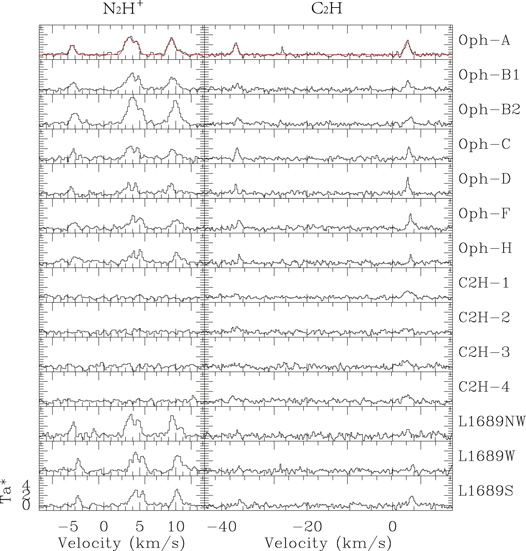
Figure 10. N2H+ and C2H spectra in the selected 14 positions. Each row is the N2H+(left) and C2H (right) spectra with the source name on the right of the C2H spectrum. The red lines show the hyperfine structure fitting results of Oph-A’s N2H+ and C2H spectra. In some C2H spectra, the peaks near −25 km s−1 are bad channels.
Download figure:
Standard image High-resolution imageTable 4. Hyperfine Line Fitting Result
| Source | Molecular | R.A. | Decl. | rms | V | Δv | Offset from N2H+ Peak | Comment |
|---|---|---|---|---|---|---|---|---|
| (J2000) | (J2000) | (K) | (km s−1) | (km s−1) | (arcsec and direction)a | |||
| Oph-A | N2H+ | 16h26m28 |
−24°23′42″ | 0.27 | 3.58(0.02) | 0.79(0.05) |
 E E |
SM1b in Oph-A |
| C2H | 16h26m28 |
−24°23′42″ | 0.26 | 3.39(0.03) | 1.11(0.05) | |||
| Oph-B1 | N2H+ | 16h27m12 |
−24°30′12″ | 0.26 | 3.75(0.02) | 0.96(0.08) |
 W W |
MM3b in Oph-B1 |
| C2H | 16h27m12 |
−24°30′12″ | 0.27 | 3.61(0.05) | 1.18(0.20) | |||
| Oph-B2 | N2H+ | 16h27m27 |
−24°27′12″ | 0.24 | 4.03(0.01) | 1.07(0.03) |

|
MM8b in Oph-B2 |
| C2H | 16h27m27 |
−24°27′12″ | 0.27 | 4.02(0.05) | 1.06(0.12) | |||
| Oph-C | N2H+ | 16h27m01 |
−24°34′42″ | 0.26 | 3.72(0.02) | 0.56(0.04) |
 SE SE |
MM6b in Oph-C |
| C2H | 16h27m01 |
−24°34′42″ | 0.28 | 3.78(0.03) | 0.71(0.04) | |||
| Oph-D | N2H+ | 16h28m29 |
−24°19′12″ | 0.28 | 3.47(0.02)c | 0.44(0.04)c |
 SE SE |
MM2b in Oph-D |
| C2H | 16h28m28 |
−24°19′12″ | 0.31 | 3.49(0.02) | 0.71(0.06) | |||
| Oph-F | N2H+ | 16h27m23 |
−24°40′42″ | 0.26 | 4.13(0.03) | 0.82(0.08) |
 W W |
MM2b in Oph-F |
| C2H | 16h27m23 |
−24°40′42″ | 0.29 | 4.23(0.04) | 1.09(0.12) | |||
| Oph-H | N2H+ | 16h27m58 |
−24°33′12″ | 0.30 | 4.18(0.03) | 0.63(0.07) |
 S S |
MM1d in Oph-H |
| C2H | 16h27m58 |
−24°33′12″ | 0.29 | 4.24(0.02) | 0.58(0.02) | |||
| L1688-C2H-1 | C2H | 16h25m39 |
−24°30′42″ | 0.24 | 3.56(0.08) | 2.08(0.18) | ||
| L1688-C2H-2 | C2H | 16h26m04 |
−24°42′42″ | 0.27 | 3.45(0.10) | 1.37(0.10) | ||
| L1688-C2H-3 | C2H | 16h24m49 |
−24°41′42″ | 0.35 | 3.00(0.15) | 2.46(0.38) | ||
| L1688-C2H-4 | C2H | 16h25m13 |
−24°51′42″ | 0.31 | 3.28(0.10) | 1.59(0.29) | ||
| L1689W | N2H+ | 16h31m39 |
−24°49′42″ | 0.31 | 4.46(0.02) | 0.59(0.04) |
 SW SW |
SMM16e in L1689-West |
| C2H | 16h31m39 |
−24°49′42″ | 0.33 | 4.57(0.09) | 0.79(0.19) | |||
| L1689S | N2H+ | 16h31m57 |
−24°57′42″ | 0.27 | 4.41(0.02) | 0.62(0.03) |
 SW SW |
SMM8e in L1689-South |
| C2H | 16h31m57 |
−24°57′42″ | 0.32 | 4.47(0.05) | 1.20(0.16) | |||
| L1689NW | N2H+ | 16h32m28 |
−24°28′42″ | 0.40 | 3.76(0.02) | 0.62(0.04) |
 S S |
SMM19e in L1689-NorthWest |
| C2H | 16h32m28 |
−24°28′42″ | 0.37 | f | f | Weak C2H emission |
Notes. CLASS fitting errors of centroid velocities and line widths are shown in the brackets behind the numbers.
aThe numbers in this column are the angular distances between the positions of the dust sources and the peaks of the N2H+ emission in the integrated intensity map. b1.3 mm dust continuum sources in Motte et al. (1998). cThe Gildas/CLASS reports that it is an optimistic fitting. d850 μm dust continuum sources in Johnstone et al. (2004). e850 μm dust continuum sources in Nutter et al. (2006). fThe line is too weak to fit the hyperfine structures.Download table as: ASCIITypeset image
L1688-C2H-1, L1688-C2H-2, L1688-C2H-3, and L1688-C2H-4 are located in the molecular ring Oph-RingSW. Their line widths are larger than those at other C2H peak positions in L1688 or L1689. The centroid velocities of L1688-C2H-3 and L1688-C2H-4 are smaller than those of any other C2H spectra at the selected positions. In these four positions, no N2H+ emission is detected. With small centroid velocities and large line widths, the C2H spectra at these four positions indicate that the molecular ring is not a part of the denser regions of L1688. In L1689NW, the C2H line is detectable but weak. For the other nine selected sources with both C2H and N2H+ spectra, the centroid velocity differences between C2H and N2H+ spectra are smaller than 0.19 km s−1, while the velocity resolutions of C2H and N2H+ spectra are 0.21 and 0.20 km s−1, respectively. In these nine positions, differences in line widths between C2H and N2H+ spectra are smaller than 0.27 km s−1, except for those of Oph-A (0.32 km s−1) and L1689S (0.58 km s−1). Such similar centroid velocities and line widths indicate that C2H N = 1–0 and N2H+ J = 1–0 trace similar gas in our observation region. Although the differences in both the centroid velocities and the line widths are similar to the channel width, from the fitting errors, the line widths of C2H are significantly larger than those of N2H+ in almost all cases, except in the positions of Oph-B2 and Oph-H. This behavior confirms our understanding that C2H traces more extended and relatively more diffuse gas than N2H+ despite their transitions having similar critical densities.
6. Conclusions
We have mapped 2.5 square degrees of the ρ-Oph MCC in the emission of the C2H N = 1–0 and N2H+ J = 1–0 transitions. The observations are the first large-scale C2H and N2H+ maps of the ρ-Oph MCC. Our main results are as follows:
- (1)Four N2H+ clumps and one C2H ring are identified and named here as Oph-J, Oph-K, Oph-L, Oph-M, and Oph-RingSW, respectively. Oph-M and the molecular ring Oph-RingSW are identified for the first time. Eight N2H+ peaks in clumps of L1688 are all co-located with dust peaks within one beam (60″).
- (2)The observed C2H-to-N2H+ ratio, [C2H]/[N2H+], varies from 5 to 110 and is little affected by the uncertainties of derived temperatures. [C2H]/[N2H+] in L1688 tends to be higher than that in L1689. For any given clump, [C2H]/[N2H+] in the inner region tends to be lower than in the outer region.
- (3)We modeled C2H and N2H+ abundances with 1D chemical models. The main difference between pure gas and gas-grain models is the dramatic drop in C2H abundance in later stages of pure gas models due to destruction by reactions with CO, which will be depleted with the presence of dust.
- (4)The diverging trends of abundances of C2H and N2H+ in our gas-grain models make [C2H]/[N2H+] a signpost of cloud conditions. For clouds with densities nH ≤ 105 cm−3, [C2H]/[N2H+] drops with time by ∼2 orders of magnitude. In the gas with a density of nH ≥ 105 cm−3 or higher, the [C2H]/[N2H+] becomes more sensitive to density.
- (5)The observed [C2H]/[N2H+] values are the results of time evolution, accelerated at higher densities. For the relatively low density regions in L1688 where only C2H emission was detected, the gas should be chemically younger.
This work is supported by National Basic Research Program of China (973 program) grant Nos. 2012CB821800 and 2015CB857101, National Science Foundation of China grant no. 11373038, and CAS International Partnership Program, grant No. 114A11KYSB20160008. We thank the anonymous referee for his or her help. This paper was improved so much with the comments and suggestions. The observation was made with the Delingha 13.7 m telescope of the Qinghai Station of Purple Mountain Observatory (see footnote 6), Chinese Academy of Sciences. We appreciate all the staff members of the observatory for their help during the observation. The telescope and the millimeter wave radio astronomy database are supported by the millimeter and submillimeter wave laboratory of PMO. D.L. acknowledges the sponsorship provided by the Guizhou Normal University and support from the CAS Interdisciplinary Innovation Team. L.Q. is supported by the FAST FELLOWSHIP. The FAST FELLOWSHIP is supported by Special Funding for Advanced Users, budgeted and administrated by Center for Astronomical Mega-Science, Chinese Academy of Sciences (CAMS). We thank Ugo Hincelin for allowing us to use the Nautilus codes. We thank Dr. Juan Li for helping us with the C2H hyperfine fittings.
Appendix A: The Critical Density Estimation Details
The critical density  is the density of molecular hydrogen at which the collisional de-excitation rate of the target molecules by hydrogen equals the spontaneous de-excitation rate of the target molecule, i.e.,

We define σ as the collisional cross section, v as the velocity of hydrogen molecules relative to target molecules, and A as the Einstein A coefficient (see next subsection). In addition, the relative velocity of hydrogen molecules can be estimated as

With these definitions, the critical density can be written as

Values of the collisional cross section can be found in BASECOL18
(Dubernet et al. 2013), which is part of the “Virtual Atomic and Molecular Data Center” (VAMDC). The spectroscopic data of BASECOL come from the CDMS (see footnote 17; the Cologne Database for Molecular Spectroscopy; Müller et al. 2001, 2005) and JPL databases19
(Pickett et al. 1998). The original data of the C2H and N2H+ collisional cross sections are from Spielfiedel et al. (2012) and Daniel et al. (2005), respectively. Tables 5 and 6 show the calculation results of critical densities ncr for C2H N = 1–0 and N2H+ J = 1–0 hyperfine lines, respectively. The critical density of N2H+ J = 1–0 can also be found in the literature, for example,  cm−3 (Tanaka et al. 2013).
Table 5. C2H N = 1–0 Critical Densities
| Transition | Rest Frequency |

|

|

|

|
|---|---|---|---|---|---|
| (MHz) | (Unit) | (Unit) | (Unit) | (Unit) | |
C2H N = 1–0 J =  – – F = 1–1 F = 1–1 |
87,284.156 |

|

|

|

|
C2H N = 1–0 J =  – – F = 2–1 F = 2–1 |
87,316.925 |

|

|

|

|
C2H N = 1–0 J =  – – F = 1–0 F = 1–0 |
87,328.624 |

|

|

|

|
C2H N = 1–0 J =  – – F = 1–1 F = 1–1 |
87,402.004 |

|

|

|

|
C2H N = 1–0 J =  – – F = 0–1 F = 0–1 |
87,407.165 |

|

|

|

|
C2H N = 1–0 J =  – – F = 1–0 F = 1–0 |
87,446.512 |

|

|

|

|
Download table as: ASCIITypeset image
Table 6. N2H+ J = 1–0 Critical Densities
| Transition | Rest Frequency |

|

|

|

|
|---|---|---|---|---|---|
| (MHz) | (Unit) | (Unit) | (Unit) | (Unit) | |
| N2H+ J = 1–0 F1 = 1–1 F = 0–1 | 93,171.621 |

|

|

|

|
| N2H+ J = 1–0 F1 = 1–1 F = 2–1 | 93,171.917 |

|

|

|

|
| N2H+ J = 1–0 F1 = 1–1 F = 1–1 | 93,172.053 |

|

|

|

|
| N2H+ J = 1–0 F1 = 2–1 F = 2–1 | 93,173.480 |

|

|

|

|
| N2H+ J = 1–0 F1 = 2–1 F = 3–1 | 93,173.777 | No Data | No Data | No Data | No Data |
| N2H+ J = 1–0 F1 = 2–1 F = 1–1 | 93,173.967 |

|

|

|

|
| N2H+ J = 1–0 F1 = 0–1 F = 1–1 | 93,176.265 |

|

|

|

|
Download table as: ASCIITypeset image
Appendix B: The Column Density Calculation Details
A simple solution to the radiative transfer equation is

where the source temperature TA, the excitation temperature Tx, and the background temperature Tbg are all modified Planck functions.
The relation between the optical depth  at the frequency ν and the molecular column density in the upper level, Nu, is

Here, Aul is the spontaneous radiative decay coefficient, c is the speed of light, h and k are the Planck and Boltzmann constants, respectively. Combining Equations (7) and (8), the Nu0, which is the column density for the molecule in the upper level, can be calculated in the Rayleigh–Jeans approximation and optically thin limits as

The total column density can be obtained after some correction (Li 2002; Qian et al. 2012),

where Fu,  , and Fb are the level correction factor, the correction factor for opacity, and the correction for the background. Fu can be written as

where Z is the partition function. The correction factor FRJ corrects for the difference between Planck’s law and the Rayleigh–Jeans limit. This difference is caused by the Taylor series expansion of  in the low column density and low-temperature assumptions.
The correction factor FRJ is

The opacity correction and background radiation correction are analyzed. The correction factor accounting for opacity is (Li 2002)

and the correction factor for background radiation is (Li 2002)

For an optically thin spectrum,  . For the correction for spectra with optical depth between 0.5 and 5, we use

Combining Equations (9), (12), (13) (or 15), and (14), the corrected column density of the molecular in the upper level, Nu, is
In our C2H and N2H+ column density calculation, we assume that the C2H and N2H+ spectra are all optically thin, the gas is in LTE, and  . Temperatures from the IRAS temperature map in COMPLETE are used as Tx, which is the excitation temperature.
  is the integrated intensity.
Table 7 shows the parameters in Equation (16). The Aul for C2H comes from Tucker et al. (1974), and the Aul for N2H+ comes from Turner (1974). Be values come from JPL Molecular Spectroscopy (Pickett et al. 1998).
Table 7. Parameters Used for Calculating Column Density
| Molecular | Frequency | Aul | Be |
|---|---|---|---|
| (GHz) | (s−1) | (MHz) | |
| C2H | 87.3486 |

|
43,674.534 |
| N2H+ | 93.1738 |

|
46,586.867 |
| Constant | k (J/K) | h (J.S) | c (m s−1) |

|

|

|
|
Download table as: ASCIITypeset image
The total column density Ntot can be calculated by

where

Here, as an approximation, we use

where the errors will be less than 1%.
These equations are for N2H+. Though the transition of C2H is N = 1–0, where N is the total angular momentum exclusive of spin, the same calculation is also suitable for C2H. One similar calculation was presented in Tucker et al. (1974) for the first detection of C2H in a number of Galactic sources.
Appendix C: The Interpolation of Including Our Observed [C2H]/[N2H+] Values in the Modeled Data
The chemical model was run with four temperatures (T1 = 10 K, T2 = 20 K, T3 = 30 K, and T4 = 40 K) and four volume densities (n1 = 5.0 × 103 cm−3, n2 = 5.0 × 103 cm−3, n3 = 5.0 × 103 cm−3, and n4 = 5.0 × 103 cm−3). For one temperature and one volume density, we obtained a set of [C2H]/[N2H+] values (namely, [C2H]/[N2H+] , with x = 1, 2, 3, or 4 the index of the temperature, y = 1, 2, 3, or 4 the index of the volume density, and z the index in the set) and corresponding chemical ages (namely,
  , with x, y, and z having the same meanings as those in [C2H]/[N2H+]
 ) from the chemical model. With the four temperatures and four volume densities, we obtained 16 sets of [C2H]/[N2H+] values and corresponding chemical ages. For an observed [C2H]/[N2H+] value, namely, [C2H]/[N2H+]oph, under the given temperature and volume density, its chemical age can be calculated by linear interpolation as

where K1 is
Here,  is the obtained chemical age, [C2H]/[N2H+]
 and [C2H]/[N2H+]
 are the abundance values that are the two values closest to the observed [C2H]/[N2H+]oph and

and  and
and  are the chemical ages corresponding to [C2H]/[N2H+]
 and [C2H]/[N2H+]
 , respectively. For the 16 sets, we have 16 values of
  in which x = 1, 2, 3, or 4 and y = 1, 2, 3, or 4. If the IRAS dust temperature of [C2H]/[N2H+]oph is Toph, the estimated chemical age of [C2H]/[N2H+]oph under one volume density is

where K2 is

Here, toph is the determined chemical age under the given volume density,  and
and  are two temperatures that are closest to Toph and

and  and
and  are two chemical ages that come from Equation (20) under the same volume density and temperatures of
  and
and  , respectively.
Footnotes
- 7
- 8
- 9
- 10
- 11
- 12
N = 1–0, J = 3/2–1/2, F = 2–1, and N = 1–0, J = 1/2–1/2, F = 1–1.
- 13
J = 1–0, F1 = 2–1, F = 2–1, J = 1–0, F1 = 2–1, F = 3–1, and J = 1–0, F1 = 2–1, F = 1–1, which are three hyperfine components in the main group.
- 14
- 15
- 16
- 17
- 18
- 19