Abstract
The Lyα Tomography IMACS Survey (LATIS) has produced large 3D maps of the intergalactic medium (IGM), providing a new window on the cosmic web at z ∼ 2.5. A key advantage of Lyα tomography is that it enables the discovery of overdense regions without the need to detect their galaxy members in spectroscopic surveys, circumventing possible selection biases. We use these maps to identify 37 IGM-selected overdensities as regions of strong and spatially coherent Lyα absorption. Simulations indicate that 85% of these are protoclusters, defined as the progenitors of z = 0 halos with mass Mdesc > 1014M⊙, and that nearly all of the rest are protogroups (1013.5 < Mdesc/M⊙ < 1014). We estimate the masses and space densities of the IGM-selected overdensities and show they are in accordance with mock surveys. We investigate the LATIS counterparts of some previously reported protoclusters, including the proto-supercluster Hyperion. We identify a new component of Hyperion beyond its previously known extent. We show that the Lyα transmission of the galaxy density peaks within Hyperion is consistent with a simple physical model (the fluctuating Gunn–Peterson approximation), suggesting that active galactic nucleus feedback or other processes have not affected the large-scale gas ionization within this structure as a whole. The LATIS catalog represents an order-of-magnitude increase in the number of IGM-selected protogroups and protoclusters and will enable new investigations of the connections between galaxies and their large-scale environments at cosmic noon.
Original content from this work may be used under the terms of the Creative Commons Attribution 4.0 licence. Any further distribution of this work must maintain attribution to the author(s) and the title of the work, journal citation and DOI.
1. Introduction
Protoclusters, the diffuse regions at z ≳ 2 destined to collapse into galaxy clusters today, play several interesting roles in the study of early galaxy evolution. They are expected to contain the most-massive halos, those where galaxy formation began the earliest and, later, where the mode of gas accretion transitioned first (R. A. Overzier 2016). Protoclusters contain a rapidly increasing fraction of the cosmic star formation rate density toward higher redshifts and likely played a key role in the reionization of the intergalactic medium (IGM; Y.-K. Chiang et al. 2017; W. Hu et al. 2021; H. Yajima et al. 2022). Toward cosmic noon, models anticipate that star formation began declining earlier and more quickly in protoclusters (S. I. Muldrew et al. 2018). By z ∼ 2, at least some systems show the hallmarks of galaxy clusters in the nearby Universe: a red sequence of galaxies and a hot gaseous medium (A. B. Newman et al. 2014; J. P. Willis et al. 2020), whose thermodynamic state in turn is affected by the galaxies evolving within it. Observations of protoclusters can inform when, where, and why galaxies and their Mpc-scale environments began to affect one other’s evolution.
In the broadest terms, such a project requires locating representative samples of protoclusters, assembling a representative inventory of their galaxy contents, measuring the physical properties of the member galaxies, and comparing these to control samples in other environments and to theoretical models. Each of these steps rapidly becomes more difficult with increasing redshift. Spectroscopic galaxy surveys can provide the most reliable determination of a galaxy’s membership in a protocluster. But particularly at z ≳ 1.5, spectroscopic samples of galaxies are generally far from mass-limited, because the identification of a redshift relies on spectral features (e.g., ultraviolet continuum, nebular line emission) whose detectability depends mainly on a galaxy’s star formation activity and dust attenuation.
Such limitations clearly make it difficult to perform a complete spectroscopic census of protocluster galaxies, including obscured galaxies and those with little or no star formation. The remarkable sensitivity of JWST can greatly improve this situation through targeted follow-up of select regions. However, wide-area surveys are still needed to locate sizable samples of protoclusters, and selection effects could also cause these surveys to miss or mischaracterize those with a substantial galaxy population that is not included in the spectroscopic selection. It is instructive that even within COSMOS, the most thoroughly observed extragalactic field for almost two decades, two protoclusters at z ∼ 3 with prominent quiescent galaxy populations were only recently uncovered (I. McConachie et al. 2022; K. Ito et al. 2023).
These considerations motivate the need for methods to discover and characterize protoclusters that complement galaxy surveys. At z ≲ 2, the detection of hot gas in an intracluster medium through its X-ray emission or the Sunyaev–Zel’dovich effect has provided such a means (e.g., M. Brodwin et al. 2011, 2012; R. Gobat et al. 2011; S. Andreon et al. 2014, 2023; A. B. Mantz et al. 2014, 2018, 2020; J. P. Willis et al. 2020; L. Di Mascolo et al. 2023). But beyond z ∼ 2.2, these methods have been much less productive, turning up one controversial example at z = 2.5 (T. Wang et al. 2016; J. B. Champagne et al. 2021).
Fortunately, the redshifted Lyα transition becomes observable from the ground at z ≳ 2. The Lyα forest absorption provides a tracer of diffuse neutral hydrogen in the IGM. By observing the Lyα transmission in a dense network of sight lines, the 3D structure of the IGM can be mapped and related to the density field, a technique known as IGM or Lyα forest tomography (C. Pichon et al. 2001; S. Caucci et al. 2008). Mapping the IGM with a resolution of several comoving megaparsecs (cMpc) in radius, roughly the typical extent of protoclusters (Y.-K. Chiang et al. 2014), requires observing the Lyα forest in the spectra of faint Lyman-break galaxies (LBGs; K.-G. Lee et al. 2014b) to achieve a commensurate sight line density. Simulations show that the resulting Lyα tomographic maps can effectively be used to locate protoclusters and to estimate their masses and evolution (C. W. Stark et al. 2015; M. Qezlou et al. 2022).
The COSMOS Lyman-Alpha Mapping and Tomography Observations (CLAMATO) survey was the first to implement the Lyα tomography technique using galaxy spectra (K.-G. Lee et al. 2014a). The CLAMATO IGM maps revealed filaments, nodes, sheets, and voids within the z ∼ 2.3 cosmic web over a volume of 4 × 10⁵h−3 cMpc3 (K.-G. Lee et al. 2018; B. Horowitz et al. 2022). Several previously known protoclusters were detected through Lyα absorption (K.-G. Lee et al. 2016, 2018). The CLAMATO maps have also been used to study the frequency and structure of cosmic voids (A. Krolewski et al. 2018).
Another approach is to use quasar spectra to sparsely sample the IGM. Z. Cai et al. (2016) showed that strong Lyα absorption spanning 15h−1 cMpc along a single line of sight is expected to be associated with large-scale matter overdensities. Contamination by high column density (HCD) absorption lines, which trace dense gas near galaxies rather than the diffuse IGM, is a major concern that can be mitigated by locating groups of several quasars that show coherent absorption. This method is expected to miss all but a tiny fraction of protoclusters (J. S. A. Miller et al. 2019), but its advantage is that enormous volumes can be surveyed to access the rarest overdensities. Indeed, the MAMMOTH survey (Z. Cai et al. 2016) based on this method has been quite successful in discovering several extremely rich protoclusters around z ∼ 2.3 (Z. Cai et al. 2017; F. Arrigoni Battaia et al. 2018; D. D. Shi et al. 2021; X. Z. Zheng et al. 2021), although follow-up observations have not always revealed a significant galaxy overdensity (Y. Liang et al. 2021).
The Lyα Tomography IMACS Survey (LATIS; A. B. Newman et al. 2020) builds on the techniques demonstrated by CLAMATO by extending them to a 10× larger volume while maintaining a comparable density of sight lines. In this paper, we will use the complete LATIS maps to identify and characterize 37 IGM-selected overdensities at z = 2.2–2.8, most of which are expected to be protoclusters. This catalog represents a roughly tenfold increase in the number of protoclusters identified independently of their galaxy populations.
Using a partially complete LATIS data set, A. B. Newman et al. (2022) investigated the regions of strongest Lyα absorption and showed that they contained fewer LBGs than expected, a deficit large enough to prevent the recognition of many of these structures in previous galaxy spectroscopic surveys. The present paper will focus on the sample of IGM-selected overdensities in the full LATIS survey and their connection to known protoclusters. In a companion paper (A. B. Newman et al. 2025; hereafter N25), we will quantify trends in the LBG content of the IGM-selected overdensities and update the A. B. Newman et al. (2022) results using the full sample.
The paper is organized as follows. We first construct IGM maps along with galaxy density maps in the three LATIS survey fields (Section 2). We then locate IGM-selected overdensities within these maps and characterize their masses and future evolution using tailored methods developed using cosmological simulations (M. Qezlou et al. 2022). We validate the resulting catalog of 37 IGM-selected overdensities and present several visualizations of these structures (Section 3). We then investigate previously reported protoclusters within our maps, especially the COSMOS field (Section 4) and the Hyperion proto-supercluster (O. Cucciati et al. 2018; also see references in Section 4.1). Throughout, we adopt the Planck Collaboration et al. (2016) cosmological parameters and report magnitudes in the AB system.
2. Data
2.1. Observations
The LATIS maps used in this paper cover the full survey area described by A. B. Newman et al. (2020), which spans 1.65 deg2 across the three fields: COSMOS and the Canada–France–Hawaii Legacy Survey (CFHTLS) D1 and D4 fields. (We also refer to COSMOS as D2 in our naming scheme since it contains the CFHTLS-D2 field.) We measure the Lyα forest in 3012 sight lines toward LBGs and QSOs comprising 4.7 × 10⁵ spectral pixels. Each pixel is a measure of the Lyα flux contrast, or transmission fluctuation, δF = F/〈F〉 − 1, where 〈F〉 represents the mean transmitted flux at each redshift. Maps are created by applying a Wiener filter to these pixels, using the dachshund code by C. W. Stark et al. (2015). We note that the output of the Wiener filter depends on the model used to describe the signal covariance, and we use the same parameters as A. B. Newman et al. (2020) and M. Qezlou et al. (2022). We smooth the Wiener filter output using a Gaussian kernel with σsm = 4h−1 cMpc, as in our previous work (A. B. Newman et al. 2020, 2022). This kernel is somewhat larger than the mean sight line separation, which varies with redshift from 〈d⊥〉 ≈ 2.5–4h−1 cMpc, which serves to increase the signal-to-noise ratio and to better match the spatial scale of protoclusters (see Section 3). We normalize the resulting 3D maps of δF by their standard deviation σmap.12 The LATIS maps span z = 2.2–2.8 with cubical voxels of 1h−1 cMpc on a side. The total volume enclosed by the survey footprint between z = 2.2 and 2.8 is 3.96 × 10⁶h−3 cMpc3 ≈ 107 cMpc3.
In addition to the IGM tomographic maps, we map the galaxy distribution. There are 2570 LBGs and QSOs with LATIS redshifts that lie within the IGM maps. Figure 1 shows the distribution of LATIS sight lines and galaxies in the D1 field in order to illustrate the level of sampling and completeness (see also A. B. Newman et al. 2020 for initial targeting statistics and A. B. Newman et al. 2025, in preparation, for full-survey statistics). To measure galaxy densities, we exclude sources without a high-confidence redshift (requiring zqual = 3 or 4; A. B. Newman et al. 2020), those that were observed only as part of “bright target” masks intended for poor observing conditions, and broad absorption line (BAL) QSOs. The LBG systemic redshifts are calibrated against transverse Lyα absorption (A. B. Newman et al. 2024). Galaxy density maps are created by weighting each galaxy by the inverse of the effective sampling rate (ESR), which is a function of the field position (A. B. Newman et al. 2024). We then convolve the resulting map by a Gaussian with σsm = 4h−1 cMpc, matching the kernel used for the IGM maps. The galaxy space density n is finally converted to an overdensity δLBG = n/〈n〉 − 1 by computing the mean density 〈n〉 within each survey field separately. This is appropriate because we found that the mean density does not vary significantly over the redshift range z = 2.2–2.8. In prior work, we referred to the galaxy overdensity as δgal, but here and in the companion paper, we use the more specific symbol δLBG, because distinctions among subpopulations are of interest. (Non-BAL quasars are also included in our maps and δLBG measures, but they comprise only 2% of the sample.) Both the IGM and LBG maps are in redshift space.
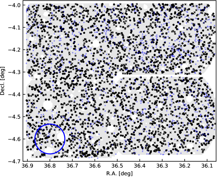
Figure 1. Map of LATIS sight lines and galaxies/QSOs in the D1 survey field. Black symbols show the 2832 targets with symbols encoding redshift range and confidence. Filled circles show Lyα sight lines along with galaxies contained within the z = 2.2–2.8 range of the tomographic maps; open squares show other galaxies with high-confidence redshifts, mostly at z < 2.2; crosses show observed galaxies for which a high-confidence redshift was not determined; and blue circles show unobserved galaxies in the photometric parent sample with r < 24.4, in the high-priority magnitude range. As discussed in A. B. Newman et al. (2020), the target sampling rate for the second-tier r = 24.4–24.8 targets is much lower. The gray background shows the survey mask, including the boundaries of the four IMACS footprints as well as untargeted regions around bright stars. The blue circle in the lower-left corner shows the FWHM of the our 4h−1 cMpc smoothing kernel at z = 2.5.
Download figure:
Standard image High-resolution imageFor quantitative estimates of δLBG, we must account for the survey boundary and unobserved regions around bright stars. We do this by convolving the survey mask by the same kernel and dividing the galaxy space density n map by the result. If this missing-volume correction factor exceeds 2, as is the case near the edges, we report no δLBG at the position. We neglect the survey mask when creating 3D visualizations of δLBG contours, since otherwise the increased noise near the survey boundary can obscure other regions.
2.2. Mock Surveys
Mock surveys that carefully mimic LATIS within cosmological simulations are essential to properly interpret the observed maps. As described by A. B. Newman et al. (2020, 2022, 2024), we primarily rely on the MultiDark Planck 2 (MDPL2) 1h−3 Gpc3 N-body simulation (A. Klypin et al. 2016), which offers a large volume but does not track gas. We estimate the Lyα transmission using the fluctuating Gunn–Peterson approximation (FGPA; J. E. Gunn & B. A. Peterson 1965; R. A. C. Croft et al. 1998; D. H. Weinberg et al. 1999). Although the FGPA is a highly simplified treatment of the IGM physics, it works well at the resolution of our tomographic maps, producing a distribution of transmission fluctuations that agrees with LATIS observations (A. B. Newman et al. 2020, 2022) and matching the relationship between Lyα transmission and matter density in magnetohydrodynamical simulations (M. Qezlou et al. 2022).
The MDPL2 mocks are created as described by A. B. Newman et al. (2022). Briefly, we use the snapshot at z = 2.535 near the midpoint of the LATIS maps. We create a suite of mock surveys by selecting nearly independent subvolumes that match the dimensions of the three LATIS survey fields. Sight lines are selected following the exact spatial distribution of the LATIS sight lines, and spectra are generated mimicking the LATIS spectral resolution, noise properties, and processing steps (see A. B. Newman et al. 2024). IGM tomographic maps are then reconstructed using a Wiener filter following the same procedures applied to the observations. We generate 100 mocks per field (COSMOS, D1, D4) and can randomly sample combinations of these to generate a larger number of survey realizations.
In addition to the mock IGM maps, we also produce mock galaxy density fields. We select mock galaxies by randomly drawing halos among those with masses  ; this threshold matches the halo autocorrelation function to that of the observed LATIS galaxies (A. B. Newman et al. 2024). The probability of a halo being selected is proportional to the ESR, evaluated at the corresponding R.A. and decl. of the survey field being mocked. Probabilities are scaled such that, on average, we select the same number of halos as LATIS galaxies that were observed in a given survey field. Halo overdensities δhalo in redshift space are then computed like the galaxy overdensities.
One application of the mock surveys is to estimate noise in the maps, which we will use to quantify the detection significance of Lyα absorption peaks and the uncertainties in some of their properties. We compare the reconstructed flux fields to a noiseless one, which is computed by directly convolving the full grid of noiseless sight lines by a Gaussian kernel (σ = 4h−1 cMpc) with no Wiener filtering. (We consider this “noiseless” in the sense that no observational noise is injected, and the sight lines are not subsampled.) The comparison is slightly complicated by the fact that the reconstructed and noiseless δF do not have an exactly one-to-one relationship, even in conditional expectation, i.e.,  and
and  (e.g., K.-G. Lee et al. 2014b; A. B. Newman et al. 2020). We find
  , where σ refers to the standard deviation of the true or reconstructed map. Using this relation, we compute the difference between the reconstructed
  and its expectation value at each voxel of each mock survey. Each mock survey thereby yields one noise realization. To evaluate the noise in the map at a given voxel, we compute the standard deviation of these differences (at the same voxel position) among all mock survey realizations.
3. A Catalog of IGM-selected Overdensities
We identify matter overdensities in the LATIS IGM maps by locating regions of strong, spatially coherent Lyα absorption. Perhaps the simplest method, which we use, is to smooth the Wiener-filtered maps (Section 2) and apply a threshold, selecting local minima of the transmitted Lyα flux where δF/σmap falls below the threshold. (Note that more negative values of δF indicate more absorption.) We refer to these local minima as Lyα absorption peaks or IGM-selected overdensities. More sophisticated techniques have aimed to reconstruct the density field and its evolution using fast simulations or analytic techniques, taking Lyα forest or galaxy survey observations as the constraints (e.g., B. Horowitz et al. 2019; M. Ata et al. 2021). Although future application of such techniques to LATIS is promising, in this initial exploration, we rely on the Wiener filtering method, which has the virtues of being simple and easily reproducible. In this section we discuss the nature of Lyα absorption peaks in simulated surveys, select a sample from the LATIS maps, quantify and evaluate their masses and densities, visualize the overdensities within the IGM and galaxy maps, and consider the robustness of the sample.
3.1. Lyα Absorption Peaks in Simulated Surveys
C. W. Stark et al. (2015) showed that smoothing and thresholding is an effective technique for identifying protoclusters in Lyα tomographic maps, given appropriate choices of the smoothing scale and the threshold δF. As mentioned in Section 2, we smooth the LATIS maps with a Gaussian having σkern = 4h−1 cMpc. This both increases the signal-to-noise ratio of the maps and approximates the average radial profile of Lyα absorption in simulated protoclusters derived by C. W. Stark et al. (2015), thus acting as a rough matched filter. C. W. Stark et al. (2015) proposed a threshold δF/σmap < −3.5 for identifying protoclusters. They found this to strike a good balance between purity and completeness. For an LATIS-like mean sight line density, mock surveys by C. W. Stark et al. (2015) indicated that 89% of the selected absorption peaks are protoclusters, defined as the progenitors of halos at z = 0 with masses >1014h−1 M⊙, and that most of the rest are nearly protoclusters.
K.-G. Lee et al. (2016) used a looser threshold δF/σmap < −3 to investigate structures in the CLAMATO maps. M. Qezlou et al. (2022) explored an even lower threshold δF/σmap < −2.35 in LATIS-like mock surveys within the IllustrisTNG300 simulation (D. Nelson et al. 2019). These surveys mimicked the main observational characteristics of LATIS (z = 2.5, representative sight line density with 〈dperp〉 = 2.7h−1 cMpc, representative noise in δF) and analysis methods (including Wiener filtering and smoothing). M. Qezlou et al. (2022) found that the strongest absorption peaks with δF/σmap < −3.5 are associated with z = 0 descendant halos that have a median virial mass Mdesc = 1014.6M⊙. Of these, 93% can be considered protoclusters based on a definition that Mdesc > 1014M⊙, indicating a high level of purity. For slightly weaker absorption peaks with −3.5 < δF/σmap < −3.0, the median is Mdesc = 1014.4M⊙, and 81% are protoclusters. Most of the peaks that “fail” to be protoclusters are nonetheless the progenitors of massive galaxy groups with Mdesc = 1013.5−14.0M⊙.
We construct our catalog of IGM-selected overdensities using Lyα absorption peaks with δF/σmap < −3. Based on the results described above, we expect this sample to be dominated by protoclusters (85%) with nearly all (98%) being protoclusters or protogroups. Rather than artificially dividing the sample into protogroup and protocluster candidates, we will present for each structure an estimate of the descendant mass at z = 0, along with the matter overdensity and mass at the observed redshift.
Although we expect the IGM-selected overdensities to comprise a reasonably pure sample of protoclusters, and a highly pure one if protogroups are included, the sample is far less complete. M. Qezlou et al. (2022) also investigated completeness using LATIS-like mock surveys: for a selection threshold of δF/σmap < −2.35, they found a detection completeness of 10%, 50%, and 90% for the progenitors of massive z = 0 halos having Mdesc/M⊙ = 1013.8, 1014.6, and 1015.0, respectively. For our purposes of building a robust catalog, we have adopted a stricter threshold, shifting the balance toward lower impurity (non-protocluster fraction) but higher incompleteness. By imposing our threshold δF/σmap < −3 on the M. Qezlou et al. (2022) analysis, we estimate a completeness of 10%, 50%, and 90% at Mdesc/M⊙ = 1014.2, 1014.8, and 1015.1. The sources of incompleteness are discussed by C. W. Stark et al. (2015) and M. Qezlou et al. (2022). Noiseless surveys fare only slightly better at the δF threshold used by M. Qezlou et al. (2022), so much of the incompleteness reflects the complex connection between the z = 2.5 Lyα flux field, as viewed 4h−1 cMpc resolution, and the assembled mass at z = 0. Our stricter δF threshold cut reduces completeness further, e.g., by 2× at Mdesc ≈ 1014.5M⊙. We emphasize that the LATIS maps contain many more significantly detected Lyα absorption peaks (e.g., −2.35 < δF/σmap < −3, corresponding to ≃3σ–5σ detection significance; see Section 3.2) than the strongest 37 peaks cataloged in Table 1, and many of these (54%) are also expected to be protoclusters.
Table 1. LATIS IGM-selected Overdensities with δF/σmap < −3
| Name | δF/σmap | R.A. | Decl. | z | Signif. | δm |

|

| Volume | Cross-IDs |
|---|---|---|---|---|---|---|---|---|---|---|
| LATIS2-D4-00 | −4.27 | 333.938 | −17.467 | 2.533 | 6.2 | 1.2 ± 0.4 | 14.92 ± 0.22 | 14.55 ± 0.35 | 2947 | ⋯ |
| LATIS2-D2-00 | −4.21 | 150.033 | 2.175 | 2.685 | 6.5 | 1.2 ± 0.4 | 15.11 ± 0.22 | 14.69 ± 0.35 | 4427 | LATIS1-D2-4, Antu |
| LATIS2-D1-00 | −4.20 | 36.202 | −4.224 | 2.452 | 6.2 | 1.3 ± 0.5 | 14.70 ± 0.22 | 14.39 ± 0.36 | 1633 | ⋯ |
| LATIS2-D2-01 | −4.09 | 149.532 | 1.974 | 2.462 | 5.0 | 1.1 ± 0.4 | 14.78 ± 0.24 | 14.45 ± 0.35 | 2098 | LATIS1-D2-1 |
| LATIS2-D2-02 | −4.02 | 149.978 | 1.970 | 2.683 | 6.3 | 1.1 ± 0.4 | 14.73 ± 0.25 | 14.42 ± 0.35 | 1933 | Antu |
| LATIS2-D2-03 | −3.97 | 150.502 | 2.173 | 2.322 | 6.3 | 1.1 ± 0.4 | 14.89 ± 0.25 | 14.53 ± 0.35 | 2719 | ⋯ |
| LATIS2-D1-01 | −3.93 | 36.203 | −4.353 | 2.455 | 6.4 | 1.1 ± 0.4 | 14.73 ± 0.26 | 14.42 ± 0.35 | 1871 | LATIS1-D1-1 |
| LATIS2-D2-04 | −3.90 | 150.332 | 2.274 | 2.457 | 6.1 | 1.1 ± 0.4 | 14.95 ± 0.26 | 14.57 ± 0.35 | 3136 | LATIS1-D2-3, Hyp |
| LATIS2-D4-01 | −3.90 | 334.100 | −17.705 | 2.595 | 6.8 | 1.0 ± 0.4 | 14.70 ± 0.26 | 14.39 ± 0.36 | 1817 | LATIS1-D4-0 |
| LATIS2-D2-05 | −3.83 | 150.474 | 2.445 | 2.473 | 5.9 | 1.0 ± 0.4 | 15.15 ± 0.27 | 14.72 ± 0.35 | 4992 | Hyp |
| LATIS2-D4-02 | −3.77 | 333.963 | −17.797 | 2.381 | 5.3 | 1.0 ± 0.4 | 14.51 ± 0.28 | 14.26 ± 0.41 | 1191 | ⋯ |
| LATIS2-D2-06 | −3.71 | 149.539 | 2.146 | 2.529 | 5.6 | 1.0 ± 0.4 | 14.63 ± 0.29 | 14.34 ± 0.38 | 1527 | ⋯ |
| LATIS2-D4-03 | −3.56 | 334.233 | −17.678 | 2.538 | 4.9 | 0.9 ± 0.4 | 14.58 ± 0.31 | 14.31 ± 0.39 | 1413 | ⋯ |
| LATIS2-D2-07 | −3.54 | 150.089 | 2.175 | 2.560 | 5.5 | 0.9 ± 0.4 | 14.32 ± 0.31 | 14.12 ± 0.45 | 750 | LATIS1-D2-0, D13 19 |
| LATIS2-D2-08 | −3.52 | 150.161 | 2.289 | 2.442 | 5.9 | 0.9 ± 0.4 | 14.72 ± 0.31 | 14.41 ± 0.36 | 1895 | L16, Hyp, CCPC* |
| LATIS2-D2-09 | −3.51 | 149.643 | 2.102 | 2.420 | 5.2 | 0.9 ± 0.4 | 14.58 ± 0.31 | 14.31 ± 0.39 | 1391 | ⋯ |
| LATIS2-D4-04 | −3.49 | 334.056 | −17.372 | 2.617 | 5.1 | 0.9 ± 0.4 | 14.21 ± 0.32 | 14.04 ± 0.48 | 596 | ⋯ |
| LATIS2-D2-10 | −3.48 | 150.330 | 2.245 | 2.497 | 5.0 | 0.9 ± 0.4 | 14.96 ± 0.32 | 14.58 ± 0.35 | 3279 | Hyp, H6 |
| LATIS2-D2-11 | −3.48 | 149.704 | 2.230 | 2.679 | 5.3 | 0.9 ± 0.4 | 14.74 ± 0.32 | 14.42 ± 0.35 | 1971 | LATIS1-D2-2, Antu |
| LATIS2-D2-12 | −3.40 | 150.046 | 2.004 | 2.500 | 4.6 | 0.9 ± 0.4 | 14.48 ± 0.33 | 14.23 ± 0.42 | 1095 | COSTCO-V |
| LATIS2-D1-02 | −3.37 | 36.138 | −4.548 | 2.568 | 5.6 | 0.9 ± 0.4 | 14.39 ± 0.33 | 14.17 ± 0.44 | 866 | LATIS1-D1-0 |
| LATIS2-D2-13 | −3.37 | 150.104 | 2.188 | 2.435 | 4.4 | 0.9 ± 0.4 | 14.57 ± 0.33 | 14.30 ± 0.39 | 1342 | L16, Hyp |
| LATIS2-D2-14 | −3.36 | 149.883 | 2.312 | 2.683 | 5.4 | 0.9 ± 0.4 | 14.37 ± 0.33 | 14.16 ± 0.44 | 831 | D13 42, Antu |
| LATIS2-D1-03 | −3.30 | 36.157 | −4.297 | 2.650 | 5.4 | 0.9 ± 0.4 | 14.63 ± 0.34 | 14.35 ± 0.38 | 1536 | ⋯ |
| LATIS2-D4-05 | −3.21 | 334.070 | −17.735 | 2.512 | 5.1 | 0.8 ± 0.4 | 14.53 ± 0.35 | 14.27 ± 0.40 | 1295 | ⋯ |
| LATIS2-D2-15 | −3.20 | 150.458 | 2.409 | 2.320 | 4.9 | 0.8 ± 0.4 | 14.61 ± 0.35 | 14.33 ± 0.38 | 1501 | D13 34 |
| LATIS2-D4-06 | −3.20 | 334.174 | −17.326 | 2.530 | 5.1 | 0.8 ± 0.4 | 14.59 ± 0.35 | 14.32 ± 0.39 | 1478 | ⋯ |
| LATIS2-D1-04 | −3.19 | 36.644 | −4.156 | 2.545 | 5.5 | 0.9 ± 0.4 | 14.39 ± 0.36 | 14.17 ± 0.44 | 892 | ⋯ |
| LATIS2-D2-16 | −3.14 | 149.677 | 2.394 | 2.681 | 4.4 | 0.8 ± 0.4 | 14.30 ± 0.36 | 14.11 ± 0.46 | 747 | Antu |
| LATIS2-D1-05 | −3.13 | 36.662 | −4.553 | 2.440 | 4.5 | 0.8 ± 0.4 | 14.22 ± 0.36 | 14.04 ± 0.48 | 599 | ⋯ |
| LATIS2-D2-17 | −3.10 | 149.934 | 1.992 | 2.549 | 4.9 | 0.8 ± 0.4 | 14.61 ± 0.37 | 14.33 ± 0.38 | 1526 | ⋯ |
| LATIS2-D1-06 | −3.08 | 36.280 | −4.234 | 2.255 | 5.7 | 0.8 ± 0.4 | 14.66 ± 0.37 | 14.36 ± 0.37 | 1690 | ⋯ |
| LATIS2-D2-18 | −3.06 | 150.559 | 2.174 | 2.479 | 5.0 | 0.8 ± 0.4 | 14.88 ± 0.37 | 14.52 ± 0.35 | 2810 | Hyp, H8 |
| LATIS2-D1-07 | −3.05 | 36.166 | −4.282 | 2.564 | 4.0 | 0.8 ± 0.4 | 14.46 ± 0.37 | 14.22 ± 0.42 | 1057 | ⋯ |
| LATIS2-D4-07 | −3.05 | 334.158 | −17.594 | 2.585 | 4.5 | 0.7 ± 0.3 | 14.26 ± 0.37 | 14.08 ± 0.47 | 699 | ⋯ |
| LATIS2-D1-08 | −3.02 | 36.490 | −4.499 | 2.360 | 5.2 | 0.8 ± 0.4 | 14.51 ± 0.38 | 14.26 ± 0.41 | 1198 | ⋯ |
| LATIS2-D2-19 | −3.00 | 150.421 | 2.001 | 2.411 | 4.6 | 0.8 ± 0.4 | 14.54 ± 0.38 | 14.28 ± 0.40 | 1305 | ⋯ |
Note. The 1σ uncertainty in δF/σmap is 0.63. Coordinate uncertainties are 2 3 in each of R.A. and decl. and 0.002 in redshift. Mass units are M⊙. The volume reported in h−3 cMpc3 is that of the watershed associated with the absorption peak (M. Qezlou et al. 2022). Notes on Cross-IDs: LATIS1 denotes strong Lyα absorption peaks discussed by A. B. Newman et al. (2022) using a previous version of the LATIS IGM maps. Antu denotes components of the extended structure described in the companion paper (N25). Hyp denotes structures within the Hyperion region, and H6/H8 denote individual peaks discussed by O. Cucciati et al. (2018). L16 = K.-G. Lee et al. (2016), COSTCO = M. Ata et al. (2022), and D13 = C. Diener et al. (2013, with ID number given).
Download table as: ASCIITypeset image
3.2. IGM-selected Overdensities in LATIS
We find 37 IGM-selected overdensities satisfying δF/σmap < −3 across the three LATIS fields (20, 9, and 8 in COSMOS, D1, and D4, respectively).13 Their properties are listed in Table 1, and their Lyα absorption and mass estimates (see below) are summarized in Figures 2 and 3. These structures show nonzero Lyα absorption with a detection significance ranging from 4.0σ–7.1σ, defined as the ratio of ∣δF∣ to the noise in the map at the position of the absorption peak (Section 2.2). The detection significance differs from δF/σmap, because σmap includes large-scale structure and is not a measure of noise.
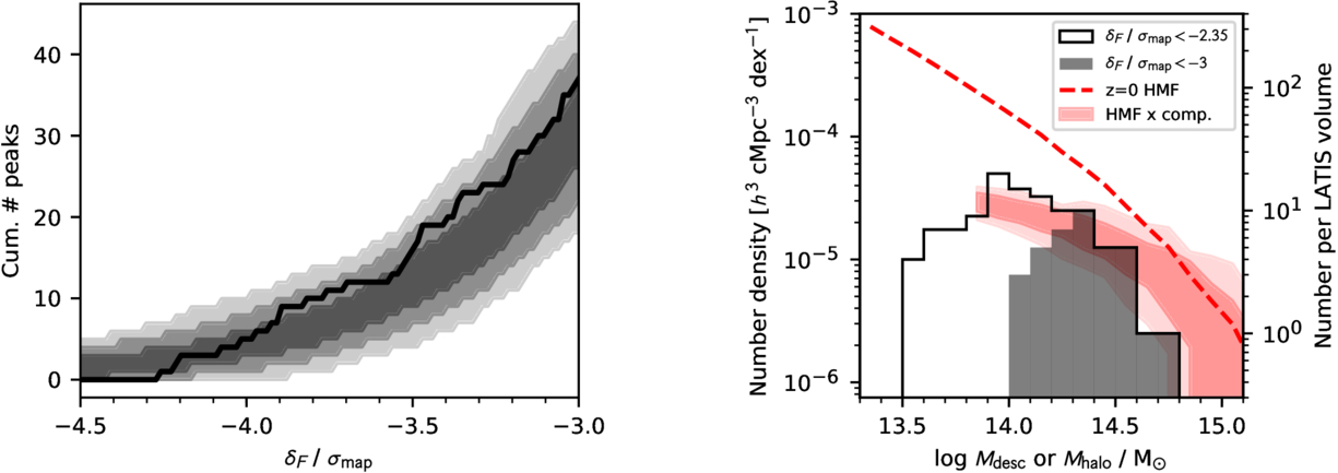
Figure 2. Left panel: the cumulative number of LATIS absorption peaks as a function of δF (solid line) is compared to the envelope of curves seen in the mock surveys (shaded regions show the central 68%, 95%, and 99.7%). Right panel: the number density of Lyα absorption peaks as a function of the estimated descendant mass Mdesc. The open histogram shows all peaks with δF/σmap < −2.35, the threshold used in the M. Qezlou et al. (2022) prescription, while the filled histogram shows the subset with δF/σmap < −3 that are the focus of this paper. The red dashed curve shows the z = 0 halo mass function from MDPL2. After weighting halos by the mass-dependent completeness computed by M. Qezlou et al. (2022; see their Figure 13) and computing the number density in many LATIS-sized subvolumes to roughly estimate cosmic variance, we obtain the red bands (enclosing the central 68% and 95% of subvolumes), which can be compared to the open histogram.
Download figure:
Standard image High-resolution image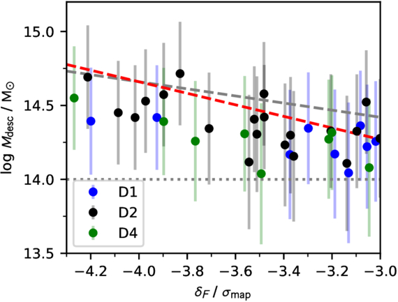
Figure 3. The Lyα flux contrast δF/σmap of the 37 IGM-selected overdensities is compared to the estimated mass Mdesc of their most-massive descendant (z = 0) halo. Protoclusters are often defined as objects with Mdesc > 1014M⊙ (above dotted line). Colors denote the three survey fields. Dashed lines show the expectation value of  conditional on δF from M. Qezlou et al. (2022, red) and K.-G. Lee et al. (2016, gray).
Download figure:
Standard image High-resolution imageWe use a naming convention similar to A. B. Newman et al. (2022): a prefix LATIS2 denoting the second catalog described in this paper (the first being A. B. Newman et al. 2022), the name of the field (note COSMOS = D2), and an integer denoting the rank order of the absorption peak within its field, sorted by δF and beginning with zero. Thus, the strongest peak in the COSMOS field in the current maps is LATIS2-D2-00.
A. B. Newman et al. (2020) tabulated only the strongest absorption peaks with δF/σmap < −3.8 in an earlier version of the maps. All of these structures, whose names begin with LATIS1, have counterparts in the current catalog, which are listed in Table 1. However, the absorption strength and thus the rank order of these structures have shifted in some cases. These shifts are due to the introduction of new observations combined with refinements to the reductions and analysis methods. These changes are detailed, including a peak-by-peak comparison, in the companion paper (N25). Here we note simply that the δF/σmap of the LATIS1 structures has increased by 0.3, on average, and that the standard deviation of the earlier and present δF/σmap measurements is 0.4; this can be compared to the random error of 0.63.
By adding noise realizations (Section 2.2) to the observed maps, we estimate uncertainties in the coordinates of the absorption peaks to be 2.7h−1 cMpc per sky coordinate and 1.5h−1 cMpc along the line of sight (1σ). These correspond to 2 3 and Δz = 0.0018 (150 km s−1), respectively, at a redshift z = 2.5.
3.3. Densities and Masses
The smoothed δF is closely related to the matter overdensity δm (e.g., K.-G. Lee et al. 2014b, 2016; M. Qezlou et al. 2022). Using the MDPL2 mocks, we find that the expectation value of δm conditional on the observed  is described by
  , where both δm and δF are smoothed with a σ = 4h−1 cMpc kernel.14
The variance about this estimator is approximately
, where both δm and δF are smoothed with a σ = 4h−1 cMpc kernel.14
The variance about this estimator is approximately  . We find that our 37 overdensities typically have δm ≈ 1, comparable to published estimates of other protoclusters when the overdensity is defined within a similar volume (e.g., C. C. Steidel et al. 1998; K. Shi et al. 2019). For comparison with other overdensity estimates, we note that our Gaussian kernel with σ = 4h−1 cMpc has the same volume as a top-hat cube with a side length of 14.7 cMpc, and so is comparable to the (15 cMpc)3 volume often used to measure protocluster overdensities (e.g., Y.-K. Chiang et al. 2014). The dispersion in the smoothed density field at z = 2.5 is
  ; thus, our sample consists of ≈3σ–5σ density fluctuations.
In addition to this point estimate of the density, the tomographic maps also contain information about the extent of structures. M. Qezlou et al. (2022) developed a method to associate empirical volumes and masses to structures in Lyα tomographic maps and to relate these to physical quantities of interest. The method defines volumes associated with absorption peaks as isocontours of δF/σmap = −2. When such a contour contains multiple absorption peaks that have δF/σmap < −2.35, the contour volume is partitioned into “watersheds” associated with each such absorption peak using a simple algorithm borrowed from image segmentation. By integrating the  relation over a watershed, a raw tomographic mass Mtomo,raw can be estimated for each structure. K.-G. Lee et al. (2016) first introduced a similar method, although the masses are not directly comparable since they used a different contour level. After applying a small 0.14 dex offset (Equation (7)) to Mtomo,raw, M. Qezlou et al. (2022) found that the resulting Mtomo is an excellent estimator (σ = 0.12 dex) of the dark matter mass MDM contained within the volume. However, the volume itself (i.e., the δF/σmap = −2 contour) is noisy, resulting in uncertainties of ≃0.3 dex compared to an ideal observation. We do not separately estimate MDM from Mtomo following Equation (8) of M. Qezlou et al. (2022), because that relation corrects a bias that becomes significant only at lower masses. For our sample, MDM ≈ Mtomo.
We report Mtomo (Table 1) as an indicator of the mass of an IGM-selected overdensity at the observed redshift, and we estimate its uncertainty as the standard deviation of masses obtained when noise realizations are added to the observed maps. We emphasize that Mtomo is defined entirely empirically as the dark matter mass enclosed within a particular contour level in a smoothed δF map. It can be used to estimate other masses (see below), but it does not have a direct numerical equality with any theoretical mass (e.g., a bound mass, the most-massive halo formed by the observed epoch or by z = 0) or any mass that would be obtained by another observational technique (e.g., a dynamical mass, or a mass estimated from a galaxy overdensity and a known bias). The masses of the IGM-selected structure span a decade, from  –15.2. We also report the volume of the watershed, i.e., the volume within a δF/σmap < −2 contour that is associated with a given absorption peak.
We use Mtomo to estimate Mdesc, the mass of the most-massive descendant halo at z = 0, using the prescription of M. Qezlou et al. (2022, Equation (9)) that follows on the work of C. W. Stark et al. (2015) and K.-G. Lee et al. (2016).15 Mtomo is larger than Mdesc, because not all material within our selected contour level will collapse into the main halo. We estimate uncertainties in Mdesc of ≃0.4 dex following M. Qezlou et al. (2022; see their Figure 11). M. Qezlou et al. (2022) showed that a noiseless tomography survey reduces the error in Mdesc by only ∼0.1 dex, and therefore much of this uncertainty is irreducible within the context of our map resolution and analysis methods. Figure 3 shows the estimated descendant masses Mdesc for each structure. The expectation value of Mdesc would place every overdensity within the protocluster regime, but the uncertainties allow an increasing probability of Mdesc < 1014M⊙ as δF increases (weaker absorption). These mass estimates and their uncertainties are consistent with our expectation that 85% of our IGM-selected overdensities are protoclusters.
Alternatively, we could estimate Mdesc directly from the peak absorption δF/σmap. Using the results of M. Qezlou et al. (2022), we built the estimator  . Figure 3 shows that the resulting Mdesc estimates would be slightly higher, by an average of 0.13 dex. This can be considered a systematic uncertainty in Mdesc, which is much smaller than the random errors for individual overdensities.
The number density of absorption peaks in the LATIS maps as a function of their strength is consistent with expectations from the MDPL2 mock surveys (Figure 2, left panel). Considering the distribution of Mdesc (right panel), we further find good agreement with the z = 0 halo mass function after multiplying it by the mass-dependent completeness determined by M. Qezlou et al. (2022; see their Figure 13). This can be seen by comparing the red bands to the open histogram, which includes all LATIS absorption peaks with δF/σmap < −2.35, the threshold used by M. Qezlou et al. (2022). The number of LATIS peaks at the highest masses  is slightly lower than the average mock survey, but still within 2σ. We therefore confirm that the abundance and masses of the IGM-selected overdensities in LATIS are consistent with cosmological expectations.
Our identification of IGM absorption-selected structures with large-scale matter overdensities relies on the Lyα absorption tracing the diffuse IGM. Strong absorption can also be produced by HCD absorption lines that are produced by dense gas close to typical galaxies, which do not necessarily indicate a 4h−1 cMpc-scale overdensity. Thus, it is important to investigate whether rare map features could be produced by HCD lines or any other features associated with an individual sight line, including data reduction artifacts. In Appendix A, we describe quantitative tests verifying that the strongest absorption peaks in LATIS are not notably sensitive to individual sight lines. In Section 5, we will discuss the possibility that locally enhanced ionization could affect the detectability of protoclusters or our estimates of their masses.
3.4. Visualizing IGM-selected Overdensities
Figure 4 depicts the LATIS IGM maps and the positions of the 37 IGM-selected overdensities within them. To better visualize the 3D large-scale structure, we provide an animation of the maps rotating about the z-axis. In addition to the IGM-selected structures identified with numbers (e.g., 1 in the COSMOS map indicates LATIS2-D2-01 in Table 1), we also show the positions of previously identified protoclusters that we will discuss in Section 4. It is visually apparent that the overdensities are clustered, as expected in hierarchical structure formation. The most striking region lines in the COSMOS (D2) field around z = 2.47, where many absorption peaks are concentrated, especially in the eastern half (low x-coordinates). This is the proto-supercluster Hyperion (see Section 4.1). The second-largest region of contiguous strong Lyα absorption lies in the COSMOS field at z = 2.68. This complex structure, which we call Antu, is discussed in the companion paper (N25). It contains five of our IGM-selected overdensities within a volume of ≈104h−3 cMpc3. In the D4 field, we note a concentration of strong Lyα absorption peaks around z = 2.53 as an interesting region for further study, which may extend beyond the region mapped by LATIS.
Figure 4. Visualizations of the IGM tomographic maps in the three LATIS survey fields, focusing on the high-density regions. Three isocontours of Lyα absorption are shown at δF/σmap = −1, −2, and −3 (from most to least transparent, and from gray to red). Axis coordinates are in units of h−1 cMpc; a conversion to redshift is shown at the top. The still image shows a projection along the y-axis. The animated version shows the maps rotating about their z-axes. LATIS overdensities listed in Table 1 are indicated by lone numbers, with larger and bolder numbers indicating the stronger absorption peaks (δF/σmap < −3.5). Other labels beginning with letters show structures identified in other studies: D (C. Diener et al. 2013), CCPC (J. R. Franck & S. S. McGaugh 2016), CC2.2 (B. Darvish et al. 2020), C (M. Ata et al. 2022, COSTCO), H (O. Cucciati et al. 2018, Hyperion) and H8 (new; Section 4.1), W16 (T. Wang et al. 2016), and L16 (K.-G. Lee et al. 2016). See Section 4 for further discussion of individual structures. We note that the x-, y-, and z-axes are aligned with -R.A., decl., and redshift, respectively and, therefore, define a left-handed coordinate system. Coordinates are displayed correctly, but the parity is inverted by ParaView, the software used to create this visualization (J. Ahrens et al. 2005).
(An animation of this figure is available.)
Download figure:
Video Standard image High-resolution imageFigure 5 shows a similar visualization focusing on the correlation between Lyα absorption and the positions of LATIS galaxies. The contours now focus on the stronger Lyα absorption regions with δF/σmap < −2, while points denote LATIS galaxies, and blue isocontours indicate a galaxy overdensity of δLBG = 3. It is visually clear that galaxies are correlated with large-scale IGM absorption, a relationship that N25 examined in detail. We find that spatial correlation between galaxies and Lyα absorption is clearer in the animation, which helps to mitigate projection effects.
Figure 5. Visualizations of the IGM tomography and galaxy density maps in the three LATIS survey fields. The Lyα absorption contours from Figure 4 are repeated here. Blue/white contours show smoothed galaxy overdensity levels of δLBG = 1 and 3. The animated version shows the maps rotating about their z-axes. See the caption of Figure 4 for information on the labels and axes.
(An animation of this figure is available.)
Download figure:
Video Standard image High-resolution imageWe complement these side-on views of the LATIS maps with an animation in Figure 6 that scans along the redshift axis. We find that this is often the most informative visualization for examining the LATIS maps in the regions around individual structures (Section 4), whereas the global visualizations in Figures 4 and 5 can provide more insight into the large-scale environment.
Figure 6. Cross sections of the three LATIS maps at fixed redshift. The animated figure scans through the full redshift range. The smoothed Lyα flux contrast δF is indicated by colors and using the dashed (δF/σmap = −2, −3, …) and solid (δF/σmap = +2, +3, …) contours. Points show the positions of LATIS LBGs and QSOs, and dotted contours show the smoothed galaxy overdensity δLBG/σ = 2, 4, 6, …, where σ is the standard deviation of the galaxy density map. Gray numbers indicate the IGM-selected overdensities cataloged in this paper (e.g., 1 in the COSMOS field is LATIS2-D2-01). Black labels and crosses indicate the positions of protocluters and protogroups in the literature. See the caption of Figure 5 for references. In the animation, we show all of the CCPC (J. R. Franck & S. S. McGaugh 2016) and C. Diener et al. (2013) structures covered by LATIS, not only the subset shown in Figure 5. Both δF and δLBG are smoothed with a Gaussian 4h−1 cMpc kernel. The left and bottom axes show the map coordinates in units of h−1 cMpc. The top and right axes give celestial coordinates R.A. and decl., respectively.
(An animation of this figure is available.)
Download figure:
Video Standard image High-resolution imageFinally, in Appendix B we provide a detailed visualization of the 3D structure of LBGs and IGM absorption surrounding the 16 strongest Lyα absorption peaks in the LATIS maps, those having δF/σmap < −3.5.
Although many IGM-selected overdensities are essentially pointlike in the LATIS maps, there are also a number of cases in which the 3D structure is resolved. Often this structure is evident in both the galaxy and IGM maps and aligns beautifully well (e.g., LATIS2-D4-00, D2-04, D1-01, and D2-08; see Appendix B). The maps also often trace connections in the cosmic web between neighboring overdensities (e.g., LATIS2-D2-00, D2-04, D2-05, and D2-08). We note a wide variety in the galaxy content of the IGM-selected overdensities, with some that are quite rich (e.g., LATIS2-D4-00, D2-03, and D2-08) and others that are remarkably poor (e.g., LATIS-D2-00, D2-05, D2-07, and D4-01). The galaxy content of the IGM-selected overdensities is the subject of the companion paper (N25).
4. Comparisons to Galaxy-selected Samples of Protoclusters
LATIS overlaps many previous searches for protoclusters and protogroups, especially within the COSMOS field, which employed a variety of different techniques. Here we briefly review several structures identified by these searches and examine their counterparts, or lack thereof, in the LATIS IGM and galaxy maps.
4.1. Hyperion
The richest region in the LATIS maps lies in the COSMOS field at z ∼ 2.45. Individual structures within this region have previously been identified as overdensities of Lyman-break galaxies (C. Diener et al. 2013), dusty star-forming galaxies (C. M. Casey et al. 2015), a radio galaxy (G. Castignani et al. 2014), distant red galaxies (DRGs; T. Wang et al. 2016), sources with photometric redshifts (Y.-K. Chiang et al. 2015), Lyα emitters (Y. Huang et al. 2022), and in one case, as a region of excess IGM absorption (K.-G. Lee et al. 2016). O. Cucciati et al. (2018) presented a unified view of the region based on LBG spectra from the VIMOS Ultra-Deep Survey (VUDS; O. Le Fèvre et al. 2015) and zCOSMOS (S. J. Lilly et al. 2007) and labeled the region as a proto-supercluster named Hyperion. Although a complete comparison of the rich structure of Hyperion as seen in galaxy and IGM maps is beyond the scope of this paper, we highlight some salient features.
O. Cucciati et al. (2018) identified seven galaxy density peaks within Hyperion labeled H1–H7 in Figures 5 and 6. We find an excellent correspondence with the LATIS galaxy density map, locating a peak near the O. Cucciati et al. (2018) coordinates for H1–H6.16 In the case of H7, to which O. Cucciati et al. (2018) ascribed the lowest mass, we do not find a distinctly separate peak from the nearby H2. Furthermore, we locate an additional galaxy density peak at coordinates (R.A., decl., redshift) = (150.459, 2.259, 2.481), close to H6, with a similar overdensity to the other Hyperion peaks (δLBG = 8 ± 2). This structure expands the previously known extent of Hyperion to the east, likely because it lies beyond the VUDS survey area. We label this new galaxy density peak as H8 and identify it with the Lyα absorption peak LATIS2-D2-18.17
In Figure 7 we compare the distribution of galaxies and Lyα absorption (panel (a)) in Hyperion. Galaxies broadly follow the IGM map, yet the positions of the O. Cucciati et al. (2018) galaxy density peaks do not correspond very closely to the Lyα absorption peaks. The highest galaxy density peak, H1 (C. M. Casey et al. 2015; O. Cucciati et al. 2018), is the heart of Hyperion in galaxy maps, but in the IGM map, H1 lies within an elongated region of absorption that is only moderately strong. It is not the strongest in the Hyperion region, and there is no clear absorption peak at its location. Among the six IGM-selected overdensities within Hyperion (see Table 1), the clearest association with the O. Cucciati et al. (2018) galaxy density peaks is of H6 with LATIS2-D2-10, but in other cases, the absorption peaks are often separated by ∼10h−1 cMpc from the nearest galaxy peak. We expect that this is, at least in part, a result of observational uncertainty in the position of a peak within a very broad region of significant Lyα absorption. In addition, there is one IGM peak that is markedly poor in LATIS galaxies: LATIS2-D2-05, which is central to Hyperion in the IGM map but contains no significant overdensity of the bright LBGs traced by LATIS at its peak.
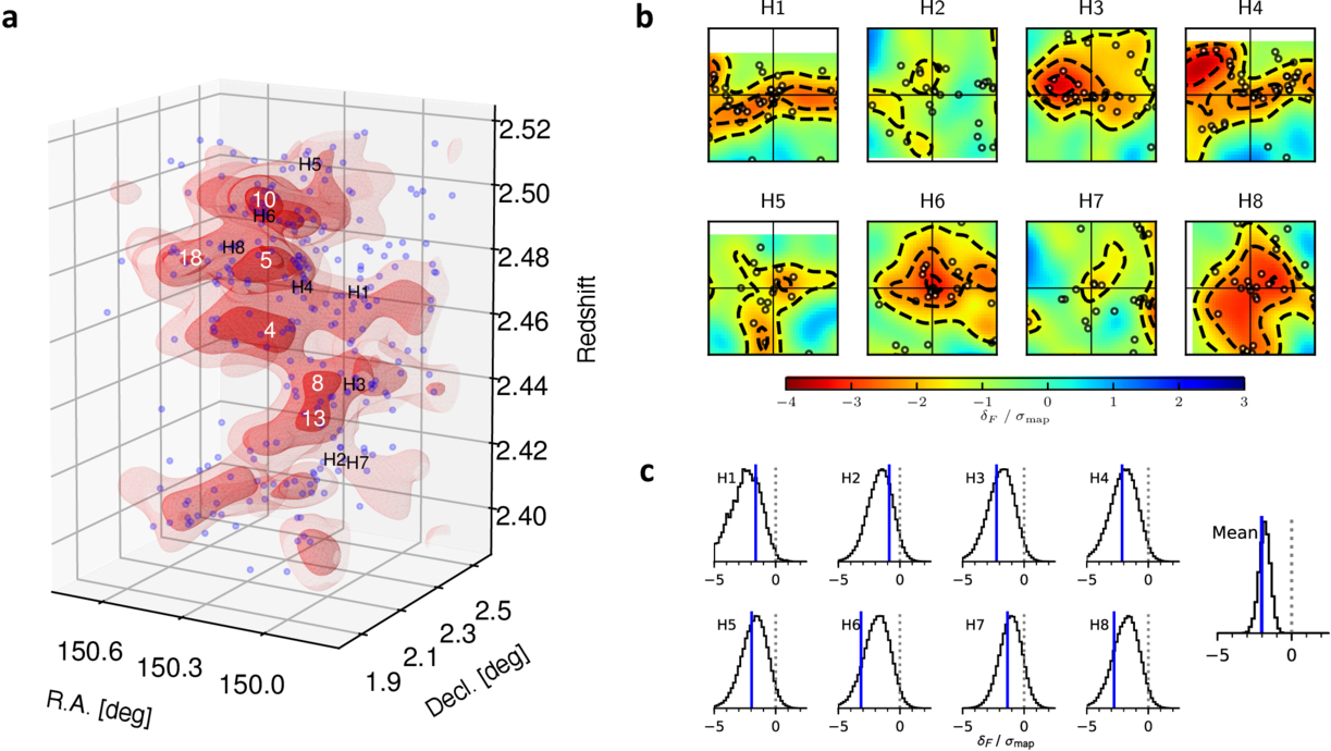
Figure 7. Panel (a): the Hyperion proto-supercluster region within the COSMOS field as traced by IGM absorption and galaxies. The three red contour levels indicate δF/σmap = −1, −2, and −3, from lightest to darkest. Blue points show the positions of LATIS galaxies. The Lyα absorption peaks are labeled with numbers, i.e., 4 indicates LATIS2-D2-04. The galaxy density peaks identified by O. Cucciati et al. (2018) are labeled H1–H7, and H8 indicates the new galaxy density peak identified with LATIS. Panel (b): for each of the eight galaxy density peaks, a cross section through the IGM map is shown. Each panel spans 40h−1 cMpc on a side, with R.A. increasing to the left and decl. toward the top. Contours indicate the δF/σmap = −1, −2, and −3 levels. Points show LATIS galaxies within ±6h−1 cMpc along the line of sight. Panel (c): for each structure H1–H8 in panel (b), the observed IGM absorption δF/σmap at the galaxy density peak position (blue vertical lines) is compared to the conditional distribution p(δF∣δLBG) from the mock surveys (black histograms). The panel labeled “Mean” shows the average 〈δF/σmap〉 over the eight peaks and the corresponding distribution in the mock surveys.
Download figure:
Standard image High-resolution imageWe now consider the compatibility of the galaxy and Lyα absorption distributions in a more quantitative way. Specifically, we examine the Lyα absorption observed at the positions of the O. Cucciati et al. (2018) galaxy density peaks along with the new H8. Panel (b) of Figure 7 shows cross sections of the IGM maps at each galaxy density peak, while panel (c) compares the observed δF/σmap at each peak to the conditional probability density function  built from the mock surveys. We observe absorption (δF < 0) at every galaxy peak, and the amount of absorption is always consistent with the FGPA-based mock surveys, evaluated in regions with matched
  . The mean 〈δF/σmap〉 over H1–H8 is better constrained than the individual peaks, with an observed value of −2.0 consistent with −1.8 ± 0.4 in the mocks.18
The FGPA assumes that the IGM gas is on a tight temperature–density relation and that the ionizing radiation field is spatially uniform; it therefore neglects any local enhancements in gas ionization due to feedback and radiation from galaxies. The concordance that we observed thus implies that gas in the Hyperion density peaks, on average and evaluated on large scales (σ = 4h−1 cMpc), has not been strongly affected by galaxy formation (see Section 5).
. The mean 〈δF/σmap〉 over H1–H8 is better constrained than the individual peaks, with an observed value of −2.0 consistent with −1.8 ± 0.4 in the mocks.18
The FGPA assumes that the IGM gas is on a tight temperature–density relation and that the ionizing radiation field is spatially uniform; it therefore neglects any local enhancements in gas ionization due to feedback and radiation from galaxies. The concordance that we observed thus implies that gas in the Hyperion density peaks, on average and evaluated on large scales (σ = 4h−1 cMpc), has not been strongly affected by galaxy formation (see Section 5).
The H5 peak was also identified by T. Wang et al. (2016) as a DRG overdensity, confirmed by Hα and CO spectroscopy. They detected extended X-ray emission and, along with other evidence, inferred the existence of a mature, collapsed cluster-sized halo of mass M200 = 1013.9M⊙. J. B. Champagne et al. (2021) argued that this X-ray emission, if it is real, does not necessarily indicate the presence of a hot diffuse medium, and is more likely to be an inverse Compton ghost, which results from the upscattering of microwave background photons by electrons in an extinguished active galactic nucleus (AGN) jet. We find a substantial galaxy overdensity (δLBG = 7 ± 2) and moderate Lyα absorption (δF = −1.8 ± 0.6) at the position of H5 that is well within the conditional distribution shown in Figure 7. This implies that cool gas is present on 4h−1 cMpc scales. However, the putative X-ray emission is detected at radii <0.4h−1 cMpc. Our observations cannot exclude a compact and hot gas phase, nor an extended multiphase structure containing both cool and hot gas.
Part of Hyperion was examined by K.-G. Lee et al. (2016) using the CLAMATO maps. They reported a system of strong absorption around z = 2.442, whose coordinates lie between LATIS2-D2-08 and LATIS2-D2-13, and thus we have recovered the same structure. We measure δF/σmap = −3.5 ± 0.6 and −3.4 ± 0.7 for these two peaks, respectively, consistent with δF/σmap = −4.0 reported by K.-G. Lee et al. (2016). They estimated that the system will form at least one cluster with mass  , consistent with our estimates (Table 1). This IGM structure overlaps H3 as well as CCPC5-z24-005 (see below).
4.2. CC2.2
B. Darvish et al. (2020) located a protocluster in the COSMOS field at z = 2.232 using narrowband Hα imaging, confirmed via Keck/MOSFIRE spectroscopy. We find a nearby LATIS galaxy overdensity (δLBG = 6 ± 2), consistent with the δgal = 6.6 ± 0.3 reported by B. Darvish et al. (2020). We detect only moderate IGM absorption of δF/σmap = −1.0 ± 0.6 at the position of the LATIS galaxy peak (δF/σmap = −1.7 ± 0.6 at the nearby absorption peak). Considering LATIS data only, the observed absorption lies easily within the conditional distribution p(δF∣δLBG) in the mock surveys, which has mean and standard deviation −1.6 ± 1.0. We explored whether the observed absorption would still be consistent with the more constrained estimate by Darvish et al., which was based on 35 Hα emitters and was evaluated over a comparable volume to the smoothing kernel that we use. Lacking more detailed information, we assume that the Hα emitter bias is similar to that of the LATIS LBGs. Even if we consider their δgal = 6.6 to be a noiseless measure, we still find that the modest observed δF is unsurprising and consistent with noise in the IGM maps.
4.3. COSTCO
M. Ata et al. (2022) used constrained cosmological simulations to reconstruct the matter density field and its evolution within COSMOS. The simulations were constrained by the galaxy density field as measured using the zCOSMOS, VUDS, MOSDEF, and ZFIRE surveys (S. J. Lilly et al. 2007; M. Kriek et al. 2015; O. Le Fèvre et al. 2015; T. Nanayakkara et al. 2016), and protoclusters were identified based on the distribution of descendant halo masses over a suite of realizations. Five new protoclusters were identified, and among these, COSTCO-I, -IV, and -V (see their Table 1) lie with the redshift range of our IGM maps. M. Ata et al. (2022) noted that their method is able to identify extended regions exhibiting mild overdensities, which may be at an earlier stage of collapse than the protoclusters typically identified by other means.
COSTCO-I was investigated by K.-G. Lee et al. (2016) and C. Dong et al. (2023) who found that the Lyα transmission in the CLAMATO maps was surprisingly high. C. Dong et al. (2023) considered this to be evidence of large-scale gas heating in this protocluster, resulting in increased ionization (see Section 5). At the location of COSTCO-I, we also find no excess Lyα absorption (δF/σmap = +0.1 ± 0.7), confirming the CLAMATO result, but we do not find a significant overdensity of LATIS galaxies.19 All of the members of the protocluster “core” were identified using MOSDEF redshifts (K.-G. Lee et al. 2016), and we find that all are fainter that the LATIS flux limit of r = 24.8.
We find similar results for COSTCO-IV: mean transmission (δF = +0.1) and no LATIS galaxy overdensity at the M. Ata et al. (2022) position. But in this case, we also do not see any clear overdensity of VUDS or zCOSMOS galaxies, and the structure is not covered by the MOSDEF and ZFIRE surveys. The putative protocluster appears very diffuse in the Ata et al. maps (see their Figure 4) and may be an example that can be identified only by using a dynamical approach.
COSTCO-V, on the other hand, is likely associated with the absorption peak LATIS2-D2-12 (δF/σmap = −3.4, δLBG = 5.2 ± 1.8).
4.4. Diener et al.
C. Diener et al. (2013) located a sample of protogroups and protoclusters in the COSMOS field using the zCOSMOS-deep spectroscopic survey. There are 21 structures in their catalog within the redshift range of the LATIS IGM maps (z = 2.2–2.8). As already shown by A. B. Newman et al. (2020), these structures, as an ensemble, are clearly overdense in the LATIS IGM and LBG maps. We find that 19 of 21 have higher-than-average galaxy density (δLBG > 0) and lower-than-average Lyα flux (δF < 0), with means of 〈δLBG〉 = 3.7 and 〈δF/σmap〉 = −1.3.
C. Diener et al. (2013) evaluated the likely descendant masses of their structures and found that it extends to halo masses as low as 1012M⊙. Thus, we do not expect to detect most of their sample in our IGM maps. We do find correspondences to IGM-selected overdensities in three cases: the Diener et al. IDs 19, 34, and 42 are LATIS2-D2-07, −15, and −14, respectively. In many other cases, a Diener et al. structure corresponds to weaker but still significant absorption in the LATIS maps, and these cases are shown in Figures 4 and 5. The animation in Figure 6 includes all of the Diener et al. structures within the LATIS footprint.
4.5. CCPC
J. R. Franck & S. S. McGaugh (2016) identified protoclusters from a compilation of public spectroscopic redshift catalogs. Within the LATIS map volume, they found five structures. CCPC-z22-006 was considered by M. Ata et al. (2022), who did not find a convincing protocluster candidate. We confirm a galaxy overdensity (δLBG = 3.0 ± 1.5) separated by 7h−1 cMpc from the CCPC coordinates (in 3D), which is accompanied by fairly strong IGM absorption (δF/σmap = −2.9 ± 0.6) just below the threshold for inclusion in our sample. CCPC-z24-005 is the highest confidence and richest of the five CCPC structures. Its reported coordinates are within 3h−1 cMpc of a strong LATIS galaxy density peak (δLBG = 7.6 ± 2.2) that overlaps LATIS2-D2-08, one of the strongest absorption peaks in LATIS (δF/σmap = −3.5 ± 0.7). Next, we find a possible counterpart of CCPC-z27-008 in the D1 field at a separation of 12h−1 cMpc, a moderate galaxy overdensity (δLBG = 3.3 ± 1.5) that overlaps a moderate IGM absorption peak (δF/σmap = −2.5 ± 0.7). We see no counterpart in either our galaxy or IGM maps for the other two structures, CCPC-z27-007 (COSMOS) and CCPC-z27-013 (D1), but we note that these were uncertain detections based on two to three galaxies.
5. Discussion
LATIS was designed to provide significant samples of over- and underdense large-scale environments at z ∼ 2.5 that are traced in a galaxy-independent manner. Its comoving volume contains, on average, ∼30 massive galaxy clusters with Mvir > 1014.5M⊙ at z = 0. The catalog presented in this paper shows that LATIS was successful in delivering a novel and sizable sample of IGM-selected overdensities. We identified 37 such overdensities by applying a threshold of δF/σmap < −3 to the smoothed Lyα transmission maps (Section 3). Using the prescriptions developed by M. Qezlou et al. (2022; and see K.-G. Lee et al. 2016), we estimated the matter overdensity and tomographic mass Mtomo of each IGM-selected overdensity at the observed redshift, along with the mass Mdesc of the largest descendant halo at z = 0.
We find that our sample comprises overdensities of δm ≈ 1, representing ≈3σ–5σ density fluctuations, with tomographic masses Mtomo = 1014.2–1015.2M⊙. They collapse into z = 0 halos with estimated masses from Mdesc = 1014.0–1014.7M⊙. The space density of IGM-selected overdensities as a function of δF or Mdesc agrees well with expectations from mock surveys (Figure 2), supporting the reliability of the mass estimates. We expect that 85% of our sample consists of protoclusters (i.e., Mdesc > 1014M⊙), a fraction that increases to 93% for the 16 strongest absorption peaks (δF/σmap < −3.5), while nearly all of the remainder are still the progenitors of massive galaxy groups (Mdesc = 1013.5−14.0M⊙; Section 3). In common with other protocluster searches, the completeness of our catalog is strong function of mass, increasing from 10%–90% as Mdesc increases from 1014.2M⊙ to 1015.1M⊙.
The LATIS catalog presented in this paper represents a roughly order-of-magnitude increase in the number of IGM-selected overdensities known. Previously, a portion of Hyperion was identified in the CLAMATO maps (K.-G. Lee et al. 2016; B. Horowitz et al. 2022). In addition, three protoclusters have been detected in IGM absorption using quasar surveys and then confirmed as high galaxy overdensities (BOSS1441, BOSS1244, and BOSS1542; Z. Cai et al. 2017; D. D. Shi et al. 2021; X. Z. Zheng et al. 2021). It is difficult to compare the Lyα absorption observed in these systems to the LATIS sample due to the different techniques used. However, their descendant masses are estimated to be Mdesc ≥ 1.4 × 10¹⁵M⊙, a range that is not accessible with an LATIS-sized volume (the expected number of such halos is 0.7). As described in Section 1, this selection technique is highly incomplete but can be deployed over enormous volumes, providing a complementary way to study the most extreme overdensities.
Our catalog opens new opportunities for studying large-scale structures at cosmic noon. An important caveat is that the catalog is a highly compressed peak-based representation of a continuous absorption field that can have complex structure. In many cases, absorption peaks are relatively isolated, and the quantities listed in Table 1 are a nearly complete summary. But in rich regions like Hyperion, which contain extended regions of absorption that connect the peaks, considering the peaks alone could be misleading. Only two of eight galaxy density peaks in Hyperion have a close counterpart in our IGM-selected catalog, which could be superficially interpreted as a gross mismatch between galaxy and IGM tracers. Yet we see that galaxies and Lyα absorption do broadly trace one another in this region, and we find statistical consistency between the expected and observed IGM absorption conditioned on the galaxy density in the Hyperion peaks. Particularly in such complex regions, it may be necessary to rely on the full IGM maps to study, for example, the variation of galaxy properties with local density.
Another important caution is that the absence of an individual protocluster from our catalog does not straightforwardly contradict its reality or its estimated mass, nor does it necessarily imply that its gas is unusually transparent to Lyα photons. Incompleteness is significant (Section 3.3), and a rather broad distribution of absorption is expected for a given measured galaxy overdensity due to noise in both measures. Reviewing the literature, we found that some previously known protoclusters have counterparts in our catalog, while a number of others showed Lyα absorption that does not meet our threshold (δF/σmap < −3) but was still significantly detected and compatible with the observed δLBG according to our mock surveys.
5.1. Possible Effects of Locally Enhanced Ionization on Protocluster Detection and Masses
Protocluster mass estimation using IGM tomography is complementary to other methods. One strength is that the IGM maps trace the full extended region of diffuse material that will collapse into a cluster-mass halo. Another is that unlike dynamical estimates derived from galaxy velocities, IGM-derived protocluster masses do not rely on any assumption of virialized equilibrium. Finally, unlike mass estimates based on galaxy overdensities, IGM-based estimates do not require knowledge of galaxy bias, and they are immune from selection effects in galaxy spectroscopic surveys that could potentially lead to environment-dependent biases in the galaxy overdensity (see Section 1; A. B. Newman et al. 2022).
On the other hand, Lyα tomography maps use neutral gas as a tracer, which represents a small fraction of the baryons. A concern is that locally enhanced ionization within protoclusters could complicate their detection and estimates of mass. Such enhanced ionization could arise from shock heated gas, induced by gravitational infall or galaxy outflows, or from an elevated intensity of ionizing radiation.
Using the IllustrisTNG300 simulation (D. Nelson et al. 2019), M. Qezlou et al. (2022) found that the transmitted Lyα flux in overdense regions, when both are smoothed to LATIS resolution, is on average very close to an FGPA-based calculation, which does not model feedback or hydrodynamics at all and assumes a spatially uniform ionizing background. In the companion paper (N25), we show that our FGPA-based mocks accurately model the mean IGM transmission as a function of density. This suggests that hydrodynamic effects in most protoclusters will minimally affect their appearance in our IGM maps.
J. S. A. Miller et al. (2021) accounted for local ionization effects using a simple model of AGN proximity zones within the IllustrisTNG100 simulation. They placed AGNs in the most-massive halos assuming a 100% duty cycle, a choice that will maximize the impact of AGN radiation on protocluster gas. They found that the ionization is indeed enhanced near massive halos, but this enhancement is confined to distances of ≲1h−1 cMpc. When the Lyα transmission is smoothed on σ = 4h−1 cMpc scales like the LATIS maps, it was little affected by the inclusion of collisional ionization or AGN photoionization in the model. The typical sensitivity of δF/σmap to these choices is ≲0.2 (see their Figure 4), 3× smaller than the measurement uncertainty in LATIS. Only in a few individual protoclusters did the models lead to differences of ΔδF/σmap ≈ 0.6, roughly equal to our measurement uncertainty. J. S. A. Miller et al. (2021) concluded that at the resolution of LATIS and similar Lyα tomography maps like CLAMATO, the uncertain ionization in protoclusters will minimally affect the completeness of protocluster discovery or mass estimates for individual systems. Systematic shifts in tomographic mass estimates were also small,  (J. S. A. Miller et al. 2021; see their Figure 4).20
C. Dong et al. (2023) presented COSTCO-I as a case study of a protocluster with unusually transparent gas, δF ≈ 0. Since, as discussed above, a large-scale (several cMpc) increase in gas ionization is not easily explained by AGN feedback as implemented in the IllustrisTNG simulations, which distribute the heating isotropically, nor by an enhanced ionizing radiation field near AGN, Dong et al. suggested that AGN jets, implemented in some cosmological simulations (R. Davé et al. 2019), could be a plausible means to heat gas over larger (several cMpc) scales. C. Dong et al. (2024) considered a broader suite of simulations and concluded that some form of AGN feedback may be needed to explain COSTCO-I and possibly several other protoclusters showing a much more modestly enhanced Lyα transmission.
Locations like COSTCO-I are important and interesting puzzles, but they appear to represent an extreme phenomenon. In most protoclusters, the gas ionization is probably not much affected by hydrodynamical effects or feedback from galaxies. As we discuss in the companion paper (N25), removing even 8% of the excess Lyα absorption from all IGM-selected overdensities would lead to a 5σ deficit in the number density of such structures. Most protoclusters thus cannot be much more transparent than we have estimated using the FGPA or IllustrisTNG.
This finding supports the validity of selecting and estimating the masses of overdensities via Lyα absorption. However, it is not inconsistent with the erasure of IGM absorption in a minority of protoclusters like COSTCO-I. Interestingly, in addition to the unusual IGM transparency, the galaxy population in COSTCO-I may also be atypical. We find that the members of its core, which were identified using MOSDEF near-infrared spectra, are all fainter than the LATIS flux limit (Section 4.3), which is uncommon for a randomly selected sample of MOSDEF galaxies at the same redshift. This points to the importance of near-infrared galaxy spectroscopy covering much larger portions of LATIS to assemble more complete samples of both galaxies and protoclusters.
5.2. Data Availability and User’s Guide
With this paper, we provide a public release of the LATIS IGM tomography maps on Zenodo21 . The release of the LATIS spectra, redshifts, and related data products will occur in an imminent separate publication, to be submitted by the end of 2025 August.
Our catalog and maps can support a variety of studies on protoclusters at cosmic noon. Several features are important to bear in mind in future applications: (1) The protocluster catalog has significant mass-dependent incompleteness (Section 3.3). Therefore, the absence of a protocluster from the catalog, which is defined by a δF/σmap < −3 threshold, is itself not very informative, although the δF value at the corresponding map position may be. (2) The positions of the IGM-selected overdensities have significant uncertainties (Table 1) that need to be taken into account when comparing to other tracers, e.g., a galaxy overdensity. In many cases, the strongest Lyα absorption peaks are embedded within a complex and extended region of absorption, and we encourage users to inspect the maps rather than relying on the peak catalog alone. (3) Comparing IGM tomography and galaxy density maps requires accounting for noise in both tracers and, ideally, reference to mock surveys.
5.3. Outlook
We have focused primarily on the IGM-derived properties of our sample. In the companion paper (N25), we consider the LBG content of these structures. The IGM maps and the catalog presented in this paper will enable a variety of other studies of environment-dependent galaxy evolution in the cosmic noon era, which we are currently pursuing (N. Chartab et al. 2025, in preparation). These include the influence of the large-scale environment on star formation, accretion and outflows as traced by galaxy metallicity, and quenching. Such work will benefit from the rich ancillary data available within the LATIS fields. In particular, we note that half of LATIS lies within COSMOS and enjoys substantial overlap with the large JWST imaging survey COSMOS Web (C. M. Casey et al. 2023) and approved spectroscopic surveys covering the same region.
Acknowledgments
This paper includes data gathered with the 6.5 m Magellan Telescopes located at Las Campanas Observatory, Chile. We gratefully acknowledge the support of the Observatory staff. A.B.N. and S.B. acknowledge support from the National Science Foundation under grant Nos. 2108014 and 2107821, respectively. B.C.L. and D.H. acknowledge support from NSF grant No. 1908422. S.B. acknowledges funding from NASA ATP 80NSSC22K1897. B.C.L. is supported by the international Gemini Observatory, a program of NSF NOIRLab, which is managed by the Association of Universities for Research in Astronomy (AURA) under a cooperative agreement with the U.S. National Science Foundation, on behalf of the Gemini partnership of Argentina, Brazil, Canada, Chile, the Republic of Korea, and the United States of America.
Appendix A: Robustness Tests
Previous studies have argued on statistical grounds that HCD lines, which we will consider as those with NHI ≳ 1017.2 cm−2, are not a major contaminant to IGM tomographic maps in which many sight lines contribute to each resolution element (K.-G. Lee et al. 2014b; C. W. Stark et al. 2015; A. B. Newman et al. 2022). To further mitigate the influence of HCD lines, we identify and mask the strongest absorption lines associated with damped Lyα systems (DLAs; A. B. Newman et al. 2024). Still, individual lines at slightly lower column densities cannot be identified at the spectral resolution of LATIS, and even a fraction of DLAs may escape detection. Thus, it remains important to investigate the sensitivity of Lyα absorption peaks, particularly the rarest and strongest, to individual sight lines.
Figure 8 demonstrates, as an example, the sight lines near the strongest Lyα absorption peak in the COSMOS map, LATIS2-D2-00. The absorption is distributed across many sight lines: 14 of 16 close sight lines show greater-than-average absorption, i.e., an average 〈δF〉 < 0 within ∣Δz∣ < 4h−1 cMpc of the peak. Thus, the absorption is spatially coherent, as expected when its origin is diffuse IGM gas, and distinct from a map signal produced by an HCD system in a single sight line. (We note that while Figure 8 illustrates the distributed nature of the absorption, the amount of absorption in the spectra cannot be straightforwardly compared to the map: the spectra and map are normalized differently, the Wiener filter weights the spectra nontrivially, and significant total weight is given to sight lines more distant than those plotted.)
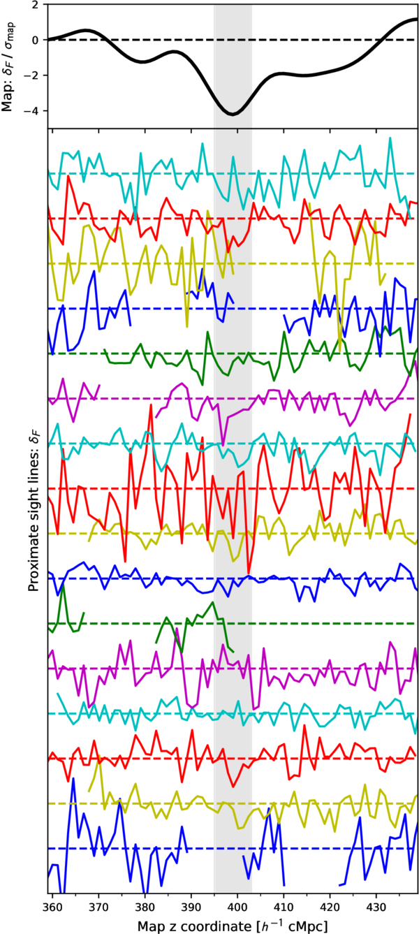
Figure 8. The top panel shows a skewer through the LATIS IGM map intersecting the Lyα absorption peak LATIS2-D2-00. The lower panel shows 16 individual sight lines close to this absorption peak, with an impact parameter d⊥ < 5h−1 cMpc. Each dashed line shows δF = 0 for the spectrum with the corresponding color; dashed lines are offset from their neighbors by 2. The vertical band shows the region within ±4h−1 cMpc of the absorption peak. Note that 14 of 16 sight lines have greater-than-average absorption (〈δF〉 < 0) in this band, demonstrating that the absorption is spatially coherent and not dominated by a single sight line.
Download figure:
Standard image High-resolution imageTurning to a quantitative examination of the full set of strong Lyα absorption peaks, A. B. Newman et al. (2022) showed that when the sight lines close to such peaks are considered, the observed distribution of the average 〈δF〉 per sight line (evaluated near the redshift of the absorption peak) matched expectations based on mock surveys constructed within IllustrisTNG300. This analysis showed no population of proximate sight lines exhibiting unexpectedly strong absorption. In addition, explicitly excising the HCD lines from the TNG mocks did not appreciably change the 〈δF〉 distribution. This indicated that the role of HCDs in producing the strong Lyα absorption peaks in the maps is expected to be negligible.
Here, we extend the A. B. Newman et al. (2022) analysis by considering the sensitivity of each of the strongest observed Lyα absorption peaks to each proximate sight line. We consider all 243 sight lines with a transverse separation <5h−1 cMpc from an absorption peak with δF/σmap < −3.5. The number of such sight lines per absorption peak ranges from 8–26, with an average of 15. Therefore, every peak is affected by an appreciable number of sight lines, which mitigates the effect of individual ones. Visual inspection indeed shows coherent widespread absorption across many sight lines, which is illustrated for one example in Figure 8.
We next reconstruct the tomographic maps by removing each of the 243 close sight lines individually, and we compute the change ΔδF at the position of the absorption peak. We then repeat this analysis in the MDPL2 mock surveys, which lack HCD lines, to understand the distribution of ΔδF that is expected from noise alone (i.e., noise in the spectra and finite sampling, but without HCD contamination). Figure 9 shows that the sensitivity of strong absorption peaks to individual sight lines agrees overall with the mock surveys and is thus well accounted for by known sources of noise. We do find two sight lines whose effect is rather strong, deepening the map absorption by 1.3–1.5 σmap. Their presence is not very unusual: two or more sight lines have a comparably strong effect in about 10% of the mock surveys. These two sight lines are near LATIS2-D2-02 and LATIS2-D4-00. Both of these are associated with strong galaxy overdensities, so there is no reason to doubt their reality, although the amount of Lyα absorption may be somewhat more uncertain in these cases.
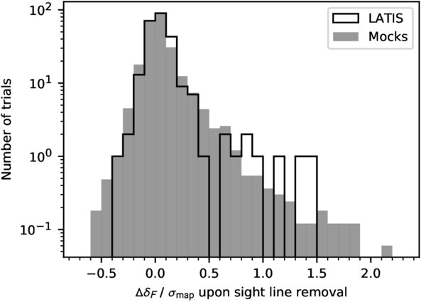
Figure 9. The sensitivity of strong absorption peaks (δF/σmap < −3.5) to individual nearby sight lines (d⊥ < 5h−1 cMpc). The solid histogram shows the changes to the map absorption strength ΔδF that result from the removal of a single such sight line. The solid histogram shows the distribution in 20 of the MDPL2-based mock surveys, normalized to match the total number of trials (i.e., close sight line removals) in the observed data set.
Download figure:
Standard image High-resolution imageAppendix B: Maps of the Strongest IGM Absorption Peaks
In Figures 10–13, we show maps of the 16 strongest Lyα absorption peaks with δF/σmap < −3.5.
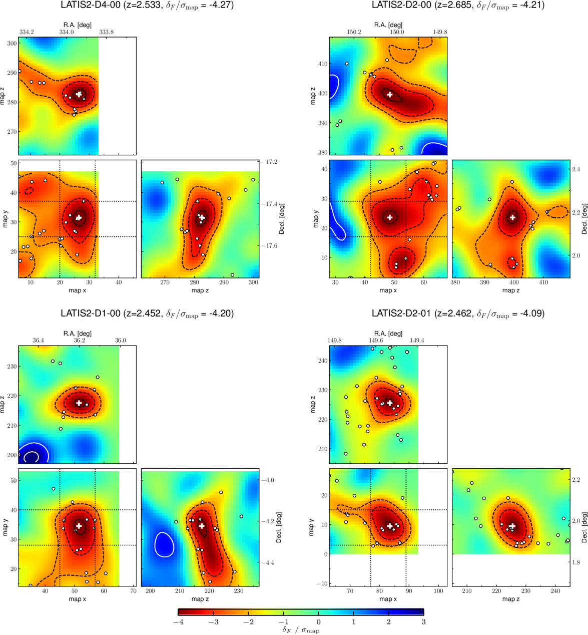
Figure 10. Visualizations of the IGM maps and galaxy distribution around the four strongest Lyα absorption peaks. For each peak, three cross sections of the IGM map through the peak are shown following the δF/σmap colorbar shown at the bottom. Dashed contours show absorption levels δF/σmap = −2, −3, …, while solid contours indicate more transparent regions with δF/σmap = +2, +3, …. Points show the positions of LATIS LBGs that lie within 6h−1 cMpc of each plane; dotted lines in the xy-projection indicate this distance from the absorption peak, which is indicated by a white cross. Map coordinates are in h−1 cMpc.
Download figure:
Standard image High-resolution image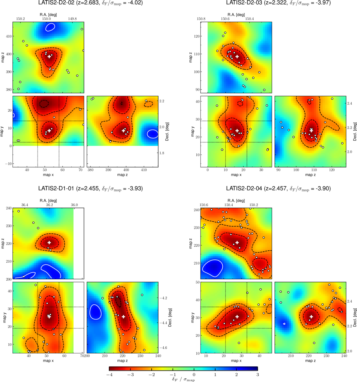
Figure 11. Continuation of Figure 10 for the next four strongest Lyα absorption peaks.
Download figure:
Standard image High-resolution image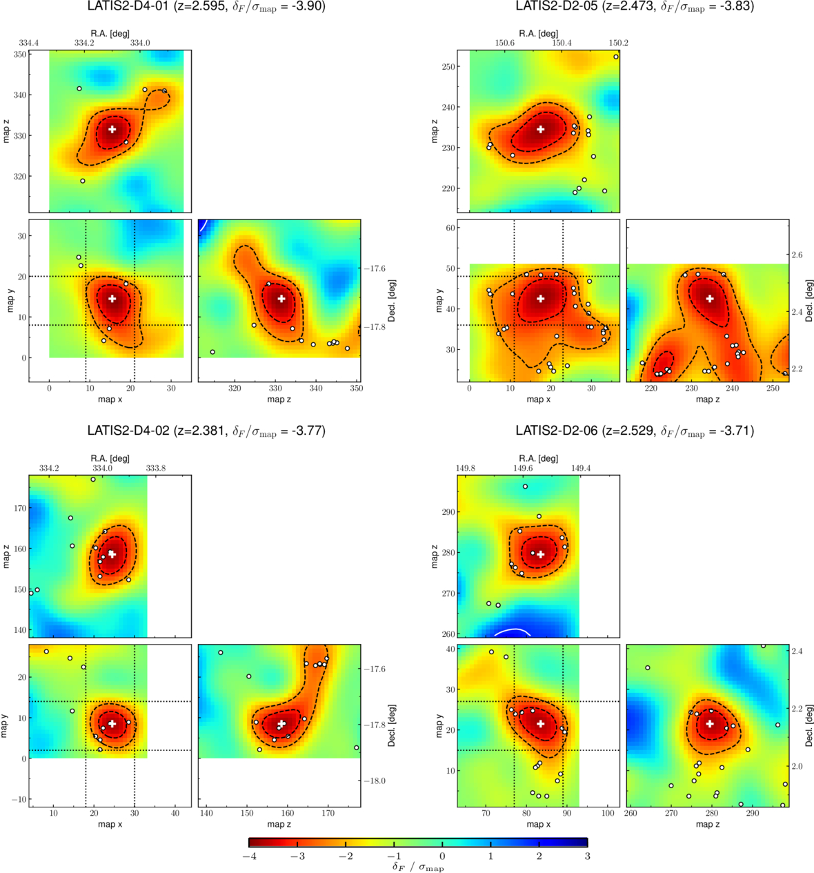
Figure 12. Continuation of Figure 11 for the next four strongest Lyα absorption peaks.
Download figure:
Standard image High-resolution image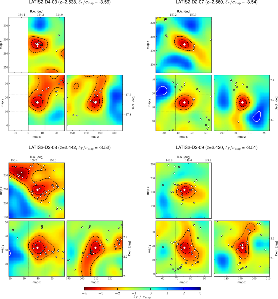
Figure 13. Continuation of Figure 12 for the next four strongest Lyα absorption peaks.
Download figure:
Standard image High-resolution imageFootnotes
- 12
σmap = 0.050, 0.048, and 0.046 in the D1, D2, and D4 fields, respectively. To mitigate edge effects, σmap is computed excluding voxels within 4h−1 cMpc of a map edge.
- 13
We made one modification to the M. Qezlou et al. (2022) prescription: we considered absorption peaks separated by less than σsm = 4h−1 cMpc to be totally blended, and we deleted the weaker peak to retain one structure in the catalog. This removed only one peak within the δF from our catalog.
- 14
This differs from the formula given by M. Qezlou et al. (2022), Equation (5), which refers to the matter overdensity evaluated in redshift space. The redshift-space overdensity is appropriate for the purpose of estimating masses from the maps, but here we provide δm in real space for easier comparison to other studies. We link voxels in the real-space δm and redshift-space δF maps using the mean line-of-sight peculiar velocity, although this correction ultimately makes little difference.
- 15
We correct an error in M. Qezlou et al. (2022), in which calculated Mtomo and MDM values were too high by approximately a factor of h−1.
- 16
The rms positional difference is only 1h−1 cMpc per coordinate, and even that may be limited by the voxel scale.
- 17
Although the galaxy and absorption peak positions are separated by 9h−1 cMpc in the sky plane, the region of strong absorption is broad and encompasses the galaxy structure.
- 18
We also considered maps in which δF and δLBG were each smoothed with a Gaussian kernel of σsm = 8h−1 cMpc (following C. Dong et al. 2023; see Section 5), larger than the σsm = 4h−1 cMpc used throughout the rest of this paper. With this larger kernel, we similarly find an observed 〈δF/σmap〉 = −2.2 that is consistent with the distribution −1.9 ± 0.3 in the mock surveys.
- 19
There is a galaxy peak with associated IGM absorption at a separation of 12h−1 cMpc, but it is a closer match to CCPC-z22-006.
- 20
J. S. A. Miller et al. (2021) contrasted their linear fit connecting δF/σmap to Mz=0 (Mdesc, in our terminology) to the one derived by K.-G. Lee et al. (2016) using the FGPA. The rather large difference suggests a large sensitivity to the astrophysics. However, we suggest that the different fitting formulae arose mostly from different choices of the independent variable (δF/σmap or
 ).
). - 21
