Abstract
Foregrounds with polarization states that are not smooth functions of frequency present a challenge to H i Epoch of Reionization (EOR) power spectrum measurements if they are not cleanly separated from the desired Stokes I signal. The intrinsic polarization impurity of an antenna’s electromagnetic response limits the degree to which components of the polarization state on the sky can be separated from one another, leading to the possibility that this frequency structure could be confused for H i emission. We investigate the potential of Faraday rotation by Earth’s ionosphere to provide a mechanism for both mitigation of and systematic tests for this contamination. Specifically, we consider the delay power spectrum estimator, which relies on the expectation that foregrounds will be separated from the cosmological signal by a clearly demarcated boundary in Fourier space and is being used by the Hydrogen Epoch of Reionization Array (HERA) experiment. Through simulations of visibility measurements that include the ionospheric Faraday rotation calculated from real historical ionospheric plasma density data, we find that the incoherent averaging of the polarization state over repeated observations of the sky may attenuate polarization leakage in the power spectrum by a factor of 10 or more. Additionally, this effect provides a way to test for the presence of polarized foreground contamination in the EOR power spectrum estimate.
1. Introduction
Experiments seeking to observe the redshifted H i signal from the Epoch of Reionization (EOR) must contend with foregrounds that are ∼104 times brighter than the cosmological signal by employing foreground removal or avoidance strategies (e.g., Santos et al. 2005; Bernardi et al. 2009, 2010; Pober et al. 2013; Dillon et al. 2014). These techniques rely on the smooth frequency structure of the foreground emission, in contrast to the spectrally structured cosmological signal (e.g., Datta et al. 2010; Morales et al. 2012; Trott et al. 2012; Pober et al. 2014; Liu et al. 2014a, 2014b; Thyagarajan et al. 2015a, 2015b). While the total intensity (Stokes I) of foreground radiation is spectrally smooth, Faraday rotation during propagation through our galaxy produces frequency structure in the linear polarization state (Stokes Q and U) at low frequencies (Jelić et al. 2010). Although extragalactic point sources appear largely depolarized, the large-scale synchrotron emission within the Milky Way appears to retain a significant level of polarization by the time it reaches an observer on Earth (Bernardi et al. 2013; Lenc et al. 2016).
The cosmological signal is expected to be effectively unpolarized given current experimental sensitivities (Babich & Loeb 2005; Hirata et al. 2018) and thus will be detected by measurements of Stokes I on the sky. On its own, frequency structure in the polarization state would not seem to be a concern when the objective is a measurement of the total intensity. However, the dipole antenna elements used in low radio frequency interferometers generally have significant sensitivity over the full sky when compared to the faintness of the EOR emission—bright foreground emission away from the antenna's boresight may still be relatively bright compared to the cosmological emission along the antenna’s boresight. Additionally, these dipole antennae are necessarily imperfect polarimeters over the full sky and do not naturally produce measurements of the incident radiation field in an orthogonal basis—a necessary condition to properly measure Stokes I. This imperfection in the measurements, commonly referred to as “polarization leakage,” means that even though we would like to obtain a pure measurement of the Stokes I intensity field on the sky, the measured visibilities will always involve a coupling to the polarization state of incident radiation. Although the sky is thought to be largely depolarized in the low-frequency radio spectrum (Farnes et al. 2014), even a polarization fraction of p ≈ 10−2, which implies a polarized brightness that is “small” compared to total intensity, is not necessarily negligible compared to the cosmological signal, and therefore has the potential to produce contamination that is comparable to the EOR signal. This coupling must be understood and appropriately addressed to ensure that frequency structure in the polarization state of astrophysical foregrounds will not be mistaken for the cosmological power spectrum.
As a successor to the PAPER experiment (Parsons et al. 2010), the Hydrogen Epoch of Reionization Array (HERA) experiment (DeBoer et al. 2017) plans to use a delay-spectrum-based estimator (Parsons et al. 2012) to make measurements of the EOR power spectrum. In contrast to other efforts to observe the EOR that pursue imaging-based methods, the delay spectrum analysis approach does not involve precision imaging and thus has not included detailed modeling and subtraction of polarized foregrounds. This makes potential contamination due to polarization leakage particularly concerning for the HERA experiment. However, in Moore et al. (2017) it was proposed that the natural density fluctuations of the plasma in Earth’s ionosphere will produce a kind of polarization filter that can attenuate the coupling of visibility measurements to the polarization state of the sky.
In this paper we seek to understand the magnitude of this ionospheric attenuation effect in visibility measurements and the derived power spectra. We simulate interferometric visibilities based on models that include the wide-field effect of the ionosphere on the polarization state of diffuse foregrounds and the full-polarization instrumental response of an early HERA antenna design. This paper is organized as follows: In Section 2, we review the relevant mathematical description of polarization in interferometric measurements including ionospheric Faraday rotation and present a pedagogical picture of its attenuating effect on the measured polarized power. In Section 3, we discuss our implementation of this formalism, which involves modeling of the instrumental response, the diffuse polarized foreground emission on the sky, and calculations using archival data of Faraday rotations based on real ionospheric behavior. Section 4 presents the results of our simulations and analysis of the effect of ionospheric behavior on HERA observations. We conclude in Section 5.
2. Preliminary Formalism
2.1. Ionospheric Variation and Polarization Attenuation
The ionosphere is a turbulent upper region of Earth’s atmosphere that is ionized by solar radiation (e.g., Kintner & Seyler 1985; Loi et al. 2015). The permeation of this ionized medium by the persistent magnetic field of Earth then produces a magnetized plasma that will induce a rotation in the linear polarization state of electromagnetic plane waves propagating through it—the effect known as Faraday rotation. The rotation angle of the electric vector is φλ2, where  is the wavelength and φ is the rotation measure (RM), which is given—in SI units—by Thompson et al. (2017):

where we have written the position vector  and φ has units of rad m−2. Here the integral is taken along the line of sight
  , the function
  is the free electron density at a radial distance s through the ionosphere, and
  is the geomagnetic field.
The primary effect of the ionosphere that has concerned EOR power spectrum measurements so far is the refractive effect of the ionosphere (Vedantham & Koopmans 2015a, 2015b), and the fact that the ionosphere is a source of thermal radio emission has also been considered in the context of 21 cm global signal measurements (Sokolowski et al. 2015). Here we are instead concerned with the effect of the ionosphere on the polarization state of the sky and with the short baselines (approximately tens of wavelengths) of the compact HERA array that are most sensitive to the large-scale cosmological signal. The polarized emission at low radio frequencies appears to be dominated by large-scale diffuse Galactic emission rather than many unresolved point sources, and the effect of small refractive shifts on such spatially smooth emission is thus expected to be negligible. We focus here on the changing Faraday rotation over months-long timescales due to variations in the ionospheric free electron density.
Driven by the heating from the Sun, the free electron density ρe varies quasi-cyclically with the rotation of Earth at any fixed geographic location—the plasma density increases when the Sun is up and decreases at night, but the ionosphere will not return to exactly the same state. This means that observations of a polarized source on the sky made on different days will always be made through an ionospheric screen that is at least slightly different than on the previous day.
Moore et al. (2017) proposed that the effect of the ionospheric Faraday rotation on polarization leakage in a visibility could be estimated by approximating the RM over the sky as a constant  and additionally that the level of polarization leakage attenuation could be estimated without regard for the details of the instrumental response. While this simple approximation turns out to be an inadequate description of real visibilities, it is equivalent to considering the effect of the ionosphere for a single source on the sky and is a good way to build some intuition. This will be useful for interpreting the results of the detailed simulations in Section 4.
Suppose you used a good polarimeter to repeatedly observe a polarized source with a linear polarization state (Q, U) on each of N different days. Propagating through the ionosphere on the nth day will rotate the polarization state by an angle  so that the observed polarization state is

where φn ∈ {φ1, …, φN} is a sequence of different ionospheric RMs toward the source on the nth day. If one then averages over all these observations, the resulting quantity would be


While this would not be a sensible thing to do if one were actually interested in measurements of the polarization state, this averaging process is realized in the standard processing of HERA visibility data for power spectrum estimation. It is straightforward to see that this decreases the magnitude of the polarization  since the magnitude of the sum in the second line is always ≤N. The ratio of the intrinsic polarized power L2 = Q2 + U2 to the power of the incoherently averaged polarization state
  is then


We can think of the varying RM as defining a set of steps in a 2D plane with unit-length steps where the position after the Nth step is

Then, the attenuation is the (squared) ratio of the actual distance traveled from the origin  to the maximum distance N that could have been traveled,

Examples of walks for several distributions of the φn values are shown in Figure 1 along with the resulting attenuation curves as a function of N. From the top, the first panel shows the walk when φn is simply a linear function

for some slope α. In this case the expression for the attenuation can be simplified by summing the geometric series


The attenuation factor is then

and the top right panel plots A2 with α = 0.02 rad m−2.
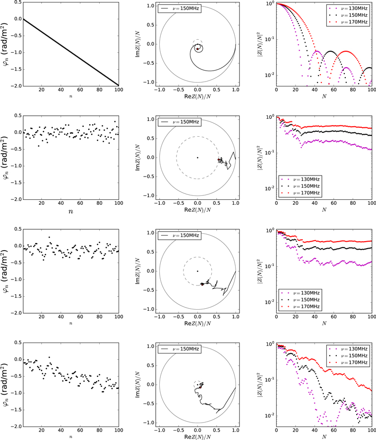
Figure 1. Examples of four different types of normalized walks Z(N)/N in the unit disk described in the text. The left panels show the path of the walk over 100 steps, while the right panels show the (squared) distance from the origin at each step—i.e., the attenuation of the polarization amplitude for a source observed through an ionospheric variation characterized by the walk in the left panel. From top to bottom the walks are generated by a linear phase angle, an uncorrelated Gaussian distributed sequence of angles, a correlated Gaussian distributed sequence, and finally the same correlated Gaussian sequence with an additional linear trend added. In the middle column the solid circle is the circle of radius 1, while the dashed circle denotes the final radius of the walk at the position Z(100)/100, which is marked by a red dot.
Download figure:
Standard image High-resolution imageThe second panel from the top shows the random walk generated by a realization of a sequence of N uncorrelated Gaussian-random variables  with σ = 0.2 rad m−2. In this case it is straightforward to compute the expectation value of the attenuation factor in Equation 4(b), which is

While the real ionospheric RM sequences of interest to us are not necessarily well described as a Gaussian-random variable or a purely linear trend, the features of these simple models are worth noting. In the case of the linear trend, the attenuation oscillates as the walk passes near the origin, but it is bounded by a  envelope. For the Gaussian distribution with finite variance σ2, the attenuation eventually approaches an asymptote
  as
as  . On the other hand, taking
  produces the limit
  , corresponding to a uniform distribution over the angle
  .
.
The third panel from the top then shows the walk generated by a sequence of correlated Gaussian-random variables  , where the covariance matrix
  is given by

Then, the panel at the bottom shows the result of adding a linear trend to the exact same φn sequence as in the third panel,  with α = 0.007 rad m−2.
These walks and the resulting attenuation curves provide some intuition for the features of the attenuation curves obtained from the more complex visibility simulations—varying degrees of smoothness, discontinuities, oscillation, and lack of consistent monotonicity in frequency. The attenuation of polarization in a visibility can then be seen as a function of each of the random walks taken by the polarization in each direction on the sky—and this function is explicitly the visibility measurement equation.
2.2. Polarization in Interferometric Visibilities and the Delay Spectrum
The fundamental measurement made by interferometric arrays is the correlation function of the electric field. The van Cittert–Zernike theorem (Born & Wolf 1999), suitably generalized to include the four possible two-point correlation functions for pairs of isolated and identical dual-feed dipole antennae (Carozzi & Woan 2009; Smirnov 2011a, 2011b), relates the polarized intensity distribution on the sky to a measured visibility matrix by


where the integral is taken over the unit sphere  (aka “the sky”). Here the vector
  denotes a baseline between the two antennas, ν is the sampled frequency,
  is a direction-dependent Jones matrix, a and b label two different antenna feed orientations, and
  is the polarized brightness field on the sky expressed as the rank-2 coherency tensor field


The symbol ⨂ denotes a tensor product of the unit vectors, and the  denotes an ensemble average of the incoherent celestial radiation fields. The functions
  are the projections of the complex-valued electric vector amplitude

of a plane wave with wavevector  and components specified in the normalized tangent basis
  induced by the equatorial coordinates R.A. α and decl. δ. As a Hermitian matrix the coherency matrix is by definition specified by the frequency- and direction-dependent Stokes parameters I, Q, U, V so that


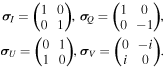
where the  matrices are the Pauli matrices
For our purposes here it is useful to adopt the point of view of a fixed observer under a rotating sky. Therefore, we will think of  as a time t dependent function, while the instrumental response of a drift-scanning antenna is fixed with respect to t. The coherency tensor is then a periodic function of the time t of the observation with a period T, which is the rotational period of Earth,

On the other hand, the ionospheric RM is only quasi-cyclic and thus not periodic in t. Since visibility data are averaged over multiple days of observation at the same local sidereal time (LST), it is useful to break the time variable into the LST t ∈ [0, T) and an integer n that indexes sidereal days. So from here on we will use the t variable to refer only to the LST of an observation. Then we write  as the visibility matrix observed on the nth sidereal day at the LST t.
The effect of the ionospheric Faraday rotation is described by a Jones matrix
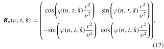
which describes the rotation  of the polarization vector
  of a plane wave upon propagation through the ionosphere. In this work we compute the visibilities resulting from

where  is the instrumental Jones matrix that describes the response of the instrument to polarized plane wave excitations. We do not include further direction-independent Jones matrices, so that our analysis concerns an idealized limit of data that has been calibrated for the direction-independent receiver-chain effects, nor do we include a thermal noise term, in order to isolate the effect of the ionospheric Faraday rotation.
From the visibilities we may form linear combinations analogous to the Stokes parameters, which we will refer to as “Vokes” parameters (e.g., “Vokes I parameter”). The Vokes parameters are

As noted in Section 1, the cosmological signal we are interested in detecting is thought to be effectively unpolarized, so Vokes I provides the highest sensitivity to the cosmological Stokes I signal, even though it is not generally a pure measurement of Stokes I. Thus, the quantity used for estimation of the power spectrum in the delay spectrum estimator is



where

are the instrumental Mueller matrix elements as shown in Figures 2 and 3, and Qn, Un are the linear polarization components after undergoing Faraday rotation in the ionosphere (Equation (2)).
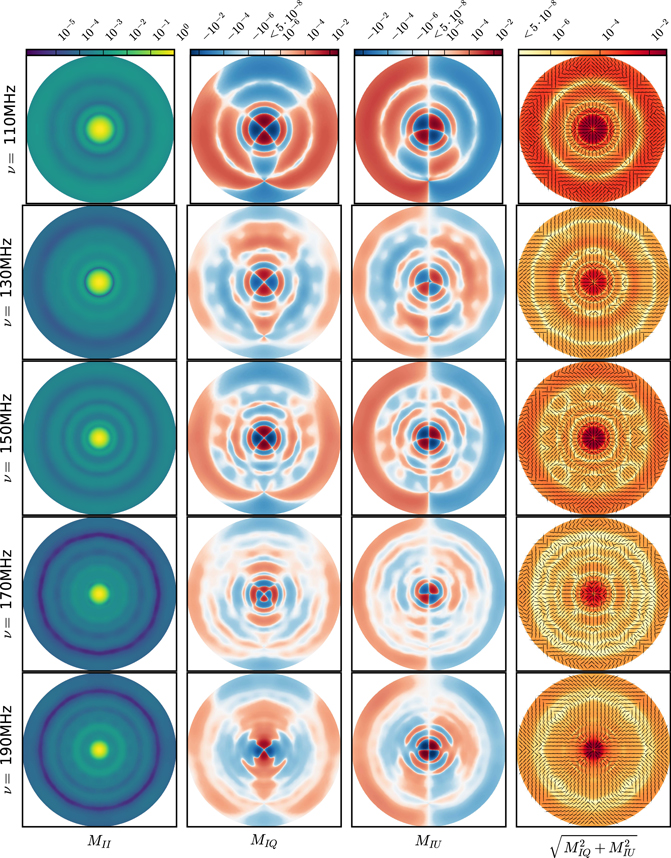
Figure 2. Mueller matrix elements for the  basis (see Appendix B) in Equation 19(c) derived from a simulation of a transmitting HERA antenna’s far-field electric vector fields. Each image is a Lambert equal-area projection of the function on the hemisphere centered on the antenna’s boresight—the inscribed circle is the antenna’s local horizon. The rows are different frequencies 110, 130, 150, 170, and 190 MHz, from top to bottom. Since the MIQ, MIU elements take values in a range that is symmetric about 0, the color scale is a symmetric log10 that spans six orders of magnitude on each side, with linearized values in the range of 10−6 to 10−8. All values are <1 in absolute value, so the sign is unambiguous. Overlaid on each image in the last column on the right is a unit tensor field that shows the geometric orientation of the polarization leakage. The plotted vector is headless and thus symmetric under a rotation by an angle π. This reflects the symmetry of the polarization state Q + iU of the source of incident radiation under a rotation by π.
Download figure:
Standard image High-resolution image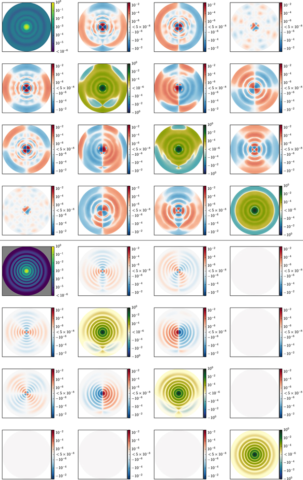
Figure 3. Mueller matrices at 150 MHz as defined in Equation (20) for the HERA model (top) and the analytically defined Airy beam dipole (bottom). As in Figure 2, the matrix elements are shown in the  basis (see Appendix B). The rows are the kernels for each of the Vokes parameters, i.e., the first row of each matrix is MII, MIQ, MIU, MIV from left to right, etc. The color scales are as described in Figure 2, but note that the diagonal elements have a different range than the off-diagonal components.
Download figure:
Standard image High-resolution imageAs an aside, it may also be useful to note that in the same way that the linear polarization on the sky may be described as a spin-2 field (in either Cartesian or polar form),

the associated Mueller matrix elements describing the polarization impurity are also the components of a spin-2 field,

The Vokes I polarization leakage terms can then be thought of as an inner product between the polarization impurity of the instrument and the polarization state Q, U of the incident radiation, which is

The right column of Figure 2 shows the scalar function MIL overlaid with a unit tensor field that shows the orientation on the sky of the instrumental impurity—geometrically, when the unit tensors of the instrumental impurity and the polarization state of the sky are at 45° (or 135° measured the other way), the inner product is 0. When the angle is 90°, the inner product is negative and minimized, i.e., MIQQ + MIUU = −MILL. The visualization in Figure 2 permitted by this representation may be useful for understanding the effect of the ionospheric Faraday rotation, which will be examined in more detail in Section 4.
The power spectrum can then be estimated from  for each baseline through the delay transform (Parsons et al. 2012)

where  is the frequency band selected to estimate the power spectrum at a given redshift and
  is a windowing function that accounts for the finite bandwidth and any further choice of tapering function. Then, an estimator
  for the spherically averaged power spectrum P(k) is obtained by averaging over time samples of the delay spectra (see, e.g., Ali et al. 2015 for the additional analysis complexities required with real measurements, and Liu et al. 2016 for more in-depth theoretical considerations),

This method of estimating the power spectrum motivates the analysis in this paper, but since we will only be considering ratios of different power spectra, the precise proportionality is unimportant here.
3. Visibility Simulation Components
We compute the visibility matrix in Equation 12(a) by a quadrature on a HEALPix1
pixelization of the sky (Górski et al. 2005). The functions  ,
,  , and
, and  are evaluated for each
  in the set of HEALPix pixels
  . Explicitly, Equation 12(a) is estimated as

where  . In this section we discuss our definition and evaluation of these three functions, as well as particular parameters of our simulations. The visibility simulation code is publicly available.2
3.1. Calculation of the Ionospheric RM from Archival Total Electron Content
Over the past three decades, methods to measure the total electron content (TEC) using global positioning system (GPS) dual-frequency receivers have been developed and improved (e.g., Royden et al. 1984; Lanyi & Roth 1988; Mannucci et al. 1998; Schaer 1999. Commission géodésique 1999; Iijima et al. 1999; Komjathy et al. 2005; Erdogan et al. 2016). These methods utilize the TEC-induced time delay between the arrival of radio waves of two closely spaced frequencies to estimate the TEC value of the ionosphere above a GPS station. Repeating this method for stations around the world and interpolating spatially provides an estimate of the TEC above any location on Earth.
Meanwhile, many generations of the International Geomagnetic Reference Field (IGRF; e.g., Finlay et al. 2010) have continually improved the model of Earth’s magnetic field. This model is composed by spatial interpolation of magnetic field measurements (in up to 13th-order spherical harmonic coefficients) reported by institutions around the world.
Based on the IonFR3
package of Sotomayor-Beltran et al. (2013), we have developed radionopy,4
a python package to calculate ionospheric RM values (the function φ in Section 2). Like IonFR, radionopy uses GPS-derived TEC maps (in the IONosphere Map EXchange format; ionex) and the IGRF to estimate the value of φ at a given latitude, longitude, and date. Unlike its predecessor, radionopy is written to calculate φ( ) over an arbitrary point set of directions on the sky, allowing images of the full sky. Additionally, radionopy implements the temporal interpolation scheme recommended in Schaer et al. (1998) to obtain full-sky maps for arbitrary times between the 2 hr time resolution of the provided IONEX data, such that the resulting φ(n, t,
  ) is a fairly smooth function of t. The interpolation scheme is as follows. Let η denote universal time (UT) and i index the times at which the TEC maps

are available as a function of the geocentric latitude θ and longitude ϕ. Then the interpolated TEC map at an arbitrary time η such that ηi ≤ η ≤ ηi+1 is a linear interpolation of the forward- and backward-rotated preceding and succeeding maps given by
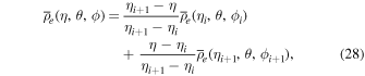
where ϕk = ϕ + ω⊕(η − ηk), with ω⊕ the angular speed of Earth. The RM function φ(n, t(η),  (θ, ϕ)) is then computed by the approximation of Equation (1) described in Sotomayor-Beltran et al. (2013). Figure 4 shows an example of radionopy output for the RM function φ(n, t,
  ) evaluated in altitude/azimuth coordinates at the location of the HERA array, and Figure 18 shows example output TEC maps over Earth.
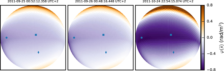
Figure 4. Images of  at a fixed LST of 2.5 hr. The first two maps are consecutive sidereal days; the third is 30 days later. At the top of each panel is the civil time and date of the RM snapshot. The images are horizon to horizon in a Lambert equal-area projection centered on longitude = +21
4283, latitude = −30
7215. The square, diamond, and circle indicate the points for which RM sequences over the day index n are shown in Figure 5. The images are oriented so that north is up and east is to the right. The places where
 correspond to points where
  ; the null to the north is near the equator.
Download figure:
Standard image High-resolution imageWhile the intrinsic time and spatial resolution of the resulting RM maps is relatively low, the RM computed in this way has recently been validated as being reasonably close to more precise measurements using pulsar timing dispersion (Malins et al. 2018).
Figure 5 shows a selection of RM sequences over 100 sidereal days at a fixed LST hour of 2.5 for several different years. The RM due to the ionosphere is generally a random function over time, with the underlying random variable being the TEC whose variation is driven by solar radiation. The RM varies randomly from day to day but follows a clear trend over the course of 100 days.
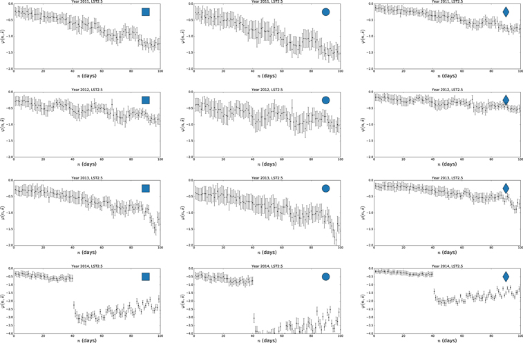
Figure 5. Rotation measure sequences over 100 days at three different points on the sky at fixed LST for each year from 2011 to 2014. The error bars are the 1σ error bars propagated from TEC uncertainties provided with the IONEX data. There is a clear trend along with the random variation. A significant solar event is observable as the large jump in 2014 (note the scale on the vertical axis of the bottom row of panels differs from the top three rows). This appears to correspond to a relatively large solar flare that was observed on 2014 October 19 by NASA’s Solar Dynamics Observatory, which was followed by several weeks of abnormally high solar activity.
Download figure:
Standard image High-resolution imageThe cause of this trend can be understood broadly by noting that the magnitude of the RM goes inversely as the time since the Sun went down. As the season progresses, a given LST transit occurs progressively closer to the previous sunset. Since the Sun is the driver of ionization in the atmosphere, as this proximity increases, the ionosphere has had less time for recombination to occur since it was last heated, resulting in a higher free electron density and thus a higher magnitude of RM.
Careful inspection of Figure 5 would reveal that each of the three different points in the RM maps is not exactly a rescaling of a common function of n, i.e., φ is not a separable function of n and  . However, it is clear in Figure 4 that there is a distinct average shape to the function
  , which is largely due to the increasing path length through the ionosphere with increasing zenith angle, as well as the projection of the geomagnetic field, along different lines of sight. These observations are quantified somewhat by considering the matrix

where
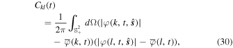

which measures the similarity in spatial structure between different days. The integral is taken over the observed hemisphere  , and the absolute value of φ is taken because the sign does not vary between days. We can also compute this correlation for the TEC by replacing φ(n, t,
  ) with
  in Equations (30) and (31). A representative example of the matrices ckl for both the RM and TEC are shown in Figure 6, where we see that the shape of the RM field is not as variable between days as the underlying TEC field.
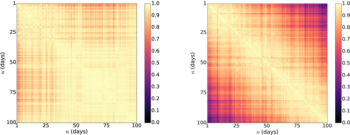
Figure 6. Left: matrices as defined in Equation (29) at t = LST 2.5 hr for 100 days starting on 2011 September 10. Right: same function as in the left panel, but applied to the TEC column density, i.e., with  replaced by
  .
.
Download figure:
Standard image High-resolution image3.2. Antenna Response Model
The instrumental Jones matrix  is derived from electromagnetic simulations of a HERA antenna element using the commercial software CST, which solves for the far-field electric field radiated by an array antenna element when operated in transmission (Fagnoni & Acedo 2016). By Lorentz reciprocity these electric field functions define the polarized response of the instrument to the incident plane waves produced by celestial sources (De Hoop 1968; Born & Wolf 1999; Potton 2004; Balanis 2005) and thus define the instrumental Jones matrix as described in Appendix B.
We take the data for the fields output by CST and interpolate to a HEALPix map. Only the simulation for a single feed is available, so we use the assumption that the antenna structure is symmetric under 90° rotations about the antenna boresight to derive the response of the second feed. Since the simulation was computed at 1 MHz resolution in frequency (which was deemed sufficient to capture the frequency structure), an interpolation in frequency is performed by cubic spline fit to the components of the spherical harmonic transforms of the electric field components and then synthesizing the fields at the desired frequency and spatial resolution. The fields simulated by CST are defined over the full sphere. We apply a hard cut to the fields at the local horizon, which is defined as the zenith angle of π/2, and set the instrumental response  to zero below this horizon.
Additionally, for comparison with a simplified model we use a Hertzian dipole with an Airy disk directivity taper. In terms of a set of Cartesian coordinates (x, y, z) such that  is along the antenna’s boresight and
  , this Jones matrix is


where J1(x) is the Bessel function of the first kind of order one and 2a = 14.6 m is the diameter of a HERA dish. The purpose of this simpler and less realistic model is to illustrate how the details of the instrumental response affect the simulations. The HERA antenna simulation used here is that of an early model that is still in the process of development. We expect that the final model of the antenna far-field response will differ slightly from the one available to us now, but not significantly so. The difference will be much smaller than the difference that can be seen in Figure 3 between the current HERA model and this simple Airy dipole construction. Further, although the polarization properties of the antenna beam have not been measured, other, more accessible properties have been measured, and their agreement with the CST simulated model suggests that it is quite realistic. Therefore, despite the similarity with the HERA model, the Airy dipole should probably be thought of as a large change to the instrument model, rather than a small one.
3.3. Sky Model
While a good model of the actual diffuse Stokes I emission is available in the form of the Global Sky Model, there is currently no equivalent full-sky model of the polarization state of the diffuse galactic synchrotron emission. Therefore, the best method available is to use a random realization generated from a statistical model with constrained parameters. We use the CORA5 code to generate a set of Stokes I, Q, and U diffuse maps. The CORA package was developed for use in Shaw et al. (2015), and the details of its physical motivation and implementation are discussed there. Briefly, CORA generates random realizations of the polarization state of the diffuse emission by RM synthesis (Brentjens & De Bruyn 2005; Jelić et al. 2010)

where F describes the distribution and polarization angle (F is a complex-valued function) of polarized emission as a function of the Faraday depth ϕ. The function F is in turn decomposed into spherical harmonic components as

The components flm(ϕ) are Gaussian-random complex-valued functions, while  is a fixed function of ϕ and
  . Realizations of diffuse linear polarization components Q, U are thus generated by drawing realizations of the components flm(ϕ). Figure 7 shows an example of the diffuse polarized power
  and polarization orientation tensor field generated by this model.
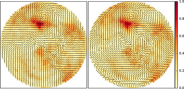
Figure 7. Image of the polarized power  in the sky model over half of the sky as would be observed by an antenna instantaneously, meaning that the edge of the image is the local horizon 90° from zenith. The linear color scale is normalized to the peak of the image, and both panels show the same map. Overlaid is a unit tensor field that shows the orientation of the linear polarization state (Q, U). The tensor field in the left panel shows the initial polarization orientation field, while the right panel shows the polarization orientation after ionospheric Faraday rotation at 150 MHz (i.e., the polarization orientation field of the polarization state (Qn, Un) in Equation 19(c)). Since the RM field
  is spatially smooth, the orientation field after Faraday rotation maintains its initial spatial correlation.
Download figure:
Standard image High-resolution imageStokes I is generated by CORA as an extrapolation of the Haslam map at 408 MHz, but we subtract the Stokes I term from the Vokes parameters when analyzing the simulated visibilities in Section 4. The one exception is in Figure 8, where, for context, we show the simulated  function including the Stokes I term.
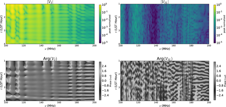
Figure 8. Amplitude and phase of  (left) and
  (right) for the intrinsic Vokes I visibility (φ = 0) computed in our fiducial visibility simulation. The amplitude plotted in both figures is relative to the maximum of
  .
.
Download figure:
Standard image High-resolution imageWhile the constraints on CORA's model parameters are, in the author’s words, “crude,” the model is sufficiently realistic to capture the important characteristic features of diffuse polarized emission, namely, the unsmooth frequency structure and spatial correlation. In particular, our results are by construction independent of the absolute level of polarized power present in the sky model and somewhat insensitive to the particular frequency spectrum of the polarization. We purposefully avoid speculation about the absolute level of polarization leakage that may be observed with HERA.
3.4. Simulation Parameters
- 1.We compute the visibility matrix for a 30 m east–west-oriented baseline.
- 2.The two dipole-feed orientations a and b are east–west and north–south, as is the case for the HERA antenna elements.
- 3.The visibilities are computed for each of 201 equally spaced frequency points ν = νj (i.e., a 0.5 MHz channel width) in the band 100–200 MHz; the smallest frequency is 100 MHz, and the largest is 200 MHz. From this band five 20 MHz sub-bands are used:

- 4.In the delay transform we use a Blackman–Harris window function.
- 5.We compute visibilities using the historical ionospheric data for the 100-day sequence starting on September 10 in each year of interest; this is the sequence for which RM data are shown in Section 3.1. The LST hour range 1–4 was chosen so that all local times in this range are between sunset and sunrise for each of the 100 days at the geographic location of the HERA array.
- 6.Fiducial simulations: We picked a single realization of the sky model to use for a set of fiducial simulations. In these simulations Nt = 96 equally spaced time samples t = tl in the LST hour range 1–4 were computed. Since each of the functions modeled in our simulation is, by construction, smooth on the scale of our sky pixelization, this is sufficient to completely sample the time dependence of the visibilities. Visibilities were computed using the historical ionosphere data from the years 2009, 2011, 2012, and 2014 and for both instrumental response models.
- 7.Sky model variance simulations: We also performed simulations using many realizations of the statistical sky model. In order to save computational time in these simulations, six equally spaced time samples were computed in the same LST range. For each of 12 yr from 2003 to 2014, visibilities for 100 different realizations of the sky model were computed, i.e., the 100 realizations are different for each year. The reduced cadence of the time sampling has an effect on the results, but we found from resamplings of the fiducial simulations that it was negligible compared to the change due to the sky model.

4. Results from Simulations
4.1. Attenuation of Linear Polarization in a Vokes Parameter Delay Spectrum
Power spectrum estimators based on the delay spectrum will generally average visibility measurements taken over multiple days at fixed (t, ν) in order to attenuate thermal noise. We follow this procedure by averaging the simulated visibilities over a set Sk of N sidereal days. The simulated visibilities  are computed on an LST grid for each of Nd consecutive days indexed by
  . We can then choose a subset
  and compute the average at fixed t as

and then the corresponding averaged Vokes parameters are

Here we find the averaging process for visibilities that was alluded to in Section 2. Now, instead of the polarization state of a single source, the averaged quantity is  , which can be considered a functional over the sequence of functions
  . For the simple model in Section 2 of a single polarized point source the notion of attenuation of the polarized power was clear, but extending the idea to the delay spectrum of visibilities warrants some additional consideration.
For each individual day n the effect of the ionospheric Faraday rotation of the polarization state on the sky is a small change to the frequency spectrum  . We can make the consequences more apparent by considering Equations (37) and (38) in greater detail. The instrumental response
  is independent of n, so we take the sum in Equation (37) inside the integral defining
  in Equation 12(a):

The sum in parentheses may always be expressed as

since the cumulative effect of summing the N different rotations may be described by a single rotation by an angle 2μ where

and an amplitude factor

which define the resultant matrix

Note that  is the matrix representation of the complex number Z(N)/N (Equation (5)). Then, for each
  the averaged Vokes
  is
is


This form exposes the fact that the ionospheric Faraday rotation need not reduce the Vokes I polarization leakage; in fact, it can increase it. Suppose that MIQQ + MIUU = 0 for some ν and some  so that the polarization leakage term is—by cosmic accident of alignment—intrinsically zero. Then, any rotation by a small angle
  will make the polarization leakage term nonzero. On the other hand, the rotation by itself can reduce the polarization leakage. Suppose now that
  . Then, there is always a choice of rotation angle 2μ that will null the polarization leakage term given by

Of course, generally the change in the magnitude of the leakage terms at each point  will fall between these two extremes, and the change in the visibility will be the result of integrating over all such changes. This may be visualized by comparing the polarization orientation of the model sky in Figure 7 and the instrumental response in Figure 2. The spatial coherence of the fields means that merely changing the polarization angle over the whole sky can have dramatic effects on the polarization leakage terms.
For small N where the ionosphere does not change very much between different days, the amplitude factor A is generally fairly close to unity, but the resultant effective rotation of the polarization state by the angle 2μ can produce a stronger (or weaker) instrumental coupling to the polarization state if the original state (Q, U) was not maximally (or minimally) aligned with the instrument. While A and  are fairly smooth functions of frequency, the change in the frequency spectrum due to the realignment term (the term proportional to
  ) including nonsmooth Q, U will tend to make the power in any given τ mode of the leakage delay spectrum fluctuate slightly. As N increases and the variation between successive ionospheric Faraday screens becomes significant, the amplitude factor A decreases enough to attenuate the polarization leakage regardless of the relative orientation of the sky’s polarization state to the instrumental response. The result is that the precise attenuation may be somewhat variable as a function of N for different τ modes, but as N increases, it should tend to converge to an overall trend. For this reason, taking the ratio of a mean over modes of the delay spectrum of the polarization leakage provides a good summary measure of the attenuation.
With these considerations in mind, we define a metric to assess the overall level of attenuation of the polarization leakage. Since we are interested in how polarization will affect power spectrum measurements, we define the attenuation in terms of the delay spectra that would be used in such measurements.
The attenuation of polarization leakage due to the ionosphere is defined as the ratio of the total power in the leakage function after averaging visibilities over different ionospheric Faraday rotations to the total power in the intrinsic leakage that would occur if the observation was made in the absence of ionosphere rotation

where  is the band over which the delay transform is computed. Then, the leakage delay power spectrum
  is computed as

and  is the delay transform (Equation (24)) of the leakage terms
  in the Vokes I visibility for the nth day:

The intrinsic leakage function  is formally obtained from Equation (47) by setting the ionospheric RM as φ = 0, so

is the Vokes I polarization leakage that would be observed without ionospheric interference and is constant as a function of n, which we think of as the intrinsic leakage.
Figures 8 shows the simulated  including the intrinsic leakage term, as well as
  on its own, and Figure 9 shows some examples of the effect of the ionospheric Faraday rotation on the frequency and delay spectra of the visibilities.
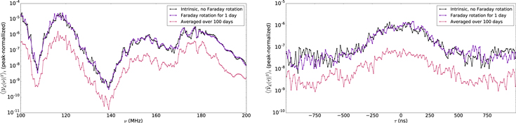
Figure 9. Left: LST-averaged square magnitude of the simulated Vokes I polarization leakage as a function of frequency ν, e.g., the result of averaging over t in the top right panel of Figure 8. Summing the black “Intrinsic” and pink “Averaged” curves over any of the sub-bands  would produce the numerator and denominator for Sk = S100 in Equation (46). Right: delay power spectra over the full 100–200 MHz band of the intrinsic Vokes I polarization leakage and a representative sample of the leakage when Faraday rotation for a single day is included. In both ν and τ representations there is a characteristic amplitude and shape, but the ionospheric Faraday rotation for a single day perturbs the spectra. The spectra resulting from averaging the visibilities over 100 days of different Faraday rotations produce an average attenuation, but additionally perturb the spectra mode by mode owing to the resultant effective rotation of the polarization state on the sky.
Download figure:
Standard image High-resolution imageIt is worth noting explicitly that by Parseval’s theorem the sums over the delay τ in Equation (46) are equivalent to simply summing the squared (and windowed) visibility amplitude over the frequency sub-band  . We write the definition in terms of delay spectra in anticipation of modifications to the definition for use with real data or more realistic simulations in which we have more confidence in the detailed frequency–frequency covariance. In particular, with real data we cannot easily subtract the Stokes I term from our Vokes I data, but we could instead apply a high-pass delay filter by restricting the sum over τ-modes in Equation (46) to
  since
since  is compact in delay compared to
  and
and  . More generally, we reiterate that the notion of “attenuation” is not uniquely defined, and we have made a particular choice here, though a well-motivated one, that is only applicable to simulated data.
In Figure 10 we plot the relative leakage factor ξI in each of five frequency bands over the 100 cumulative subsets Sk of S, the set of 100 different days for which visibilities were simulated. The cumulative subsets are  , so in Figure 10 we can write the attenuation ξI as a function of N, the number of consecutive sidereal days in the sum. This will be referred to as the “natural attenuation,” since it is “natural” to simply average up all available data after observing for N days. Each panel shows the set of five such discrete attenuation curves for each of the four calendar years and two instrumental response models for which we computed visibilities as discussed in Section 3.
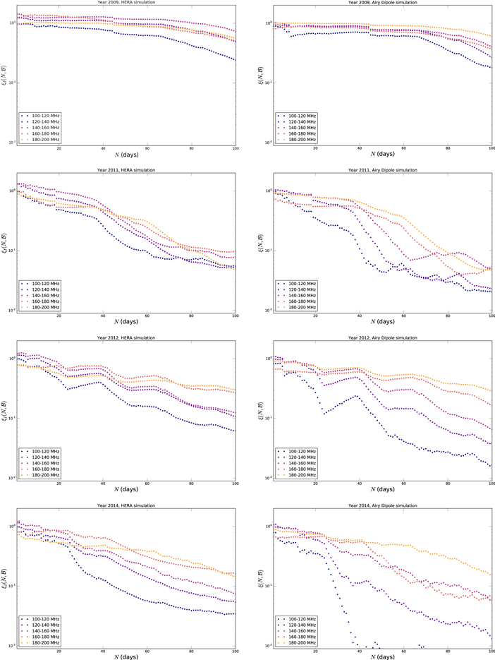
Figure 10. Natural attenuation of the Vokes I polarization leakage as defined in Equation (46) as a function of the number N of consecutive days averaged over, up to 100 days from September 10 for the four years 2009, 2011, 2012, and 2014. Left: from the fiducial simulations with the HERA antenna response model. Right: from the fiducial simulations with the simple Airy dipole model. It is interesting to see that the large change in the magnitude of the RM during the year 2014 (Figure 5) does not produce a correspondingly large change in the attenuation.
Download figure:
Standard image High-resolution imageThe smooth nature of the attenuation curves is reminiscent of the correlated and trending walks in the plane considered in Section 2 and reflects the trends of φ(n) shown in Figure 5. We can also recognize the occasional oscillatory behavior as a natural feature of the polarization state undergoing a trending walk in the tangent plane at each point on the sky. The effect of the changing relative orientation of the polarization state to the instrumental response is evident as ξI > 1 for some of the curves when N is small.
The lack of uniform ordering by frequency band is due to the interplay between the intrinsic oscillation in the random walk of the polarization state and the frequency dependence of the instrumental coupling over each band  . Although the instrumental response changes only slowly over each 20 MHz sub-band, we see that there is significant variation in Figure 2 over the full 100–200 MHz band. This contributes to the deviations from the ordering of attenuation curves by central frequency that we might naively expect from the simple formulae in Section 2. Additionally, there is the changing relative importance of the factor A and the μ-rotation as a function of N. For small N, the amplitude factor A ∼ 1, but for the highest-frequency band the rotation is changing the relative polarization angle between the sky and the instrumental response such that the Faraday-rotated leakage is smaller in magnitude than the intrinsic leakage. This is in contrast to the lower-frequency bands, some of which have the leakage amplified (ξI > 1) somewhat by the μ-rotation for small N. As N increases, the amplitude factor A becomes more significant. In particular, the magnitude of A decreases more quickly at lower frequencies. As a result, eventually the attenuation curves of the lower-frequency bands drop into a monotonic, or nearly monotonic, ordering with frequency band. Of course, μ is still a function of N, so its variation should be expected to contribute to eccentricities in the curves as the alignment of the effective polarization state to the instrumental response continues to gradually change.
The attenuation curves for the HERA model show that in 100 days the polarization leakage in our simulations is attenuated by a factor of 10 or more in the three bands in the 100–160 MHz range, and the two higher-frequency bands are not far behind. Comparison with the Hertzian dipole model shows that the details of the coupling between the instrument and the polarization state of the sky do affect the resulting visibility enough to noticeably change the attenuation factor as a function of N. This makes clear that accurate prediction of the attenuation factor is dependent on an accurate beam (and sky) model.
4.2. Sky Model Variance
There is significant variation in the natural attenuation curves with the changing ionospheric Faraday rotations for different years, which reflects the underlying variation of the visibilities. The fact that different rotations of the polarization state of the sky can produce such a change in the power spectrum suggests that if the Faraday rotation field and instrument model are held fixed, different polarized skies could also produce significantly different results.
The attenuation curves we have considered so far are the results of simulations using a single realization of a statistical model of the diffuse polarization. To understand how much our simulations could vary with the choice of sky model, we compute visibilities for 100 realizations of the diffuse polarization generated with CORA.
Figures 11–13 show the resulting natural attenuation curves of 100 different sky model realizations using the HERA instrument model over the same 100-day sequence in each year from 2003 to 2014. For each year and sub-band the geometric mean and geometric variance of the sample of attenuation curves are estimated, and the resulting mean curve and 2σ intervals are also shown.
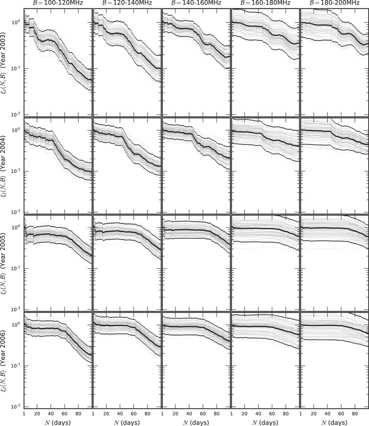
Figure 11. Distributions of the Vokes I polarization leakage attenuation factor obtained in simulations with different realizations of the sky model. For each year (row) 100 different sky realizations are generated and the attenuation factor is computed in each sub-band (column). Each thin gray curve is the attenuation curve for a realization of the sky model. The thick black points show the geometric mean and geometric 2σ deviation of the distribution of ξI(N) for each N.
Download figure:
Standard image High-resolution image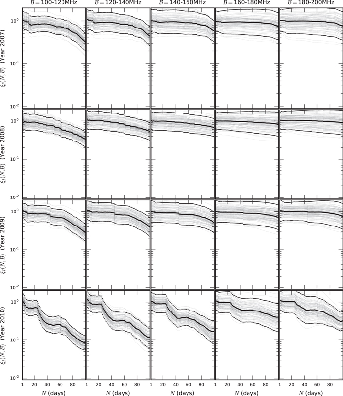
Figure 12. Same as in Figure 11, but for the years 2007–2010.
Download figure:
Standard image High-resolution image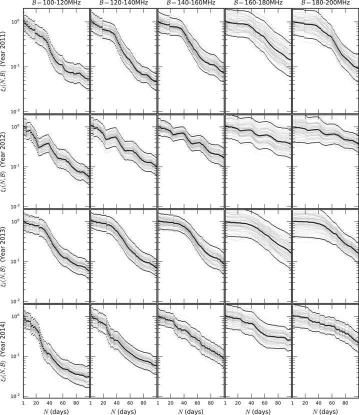
Figure 13. Same as in Figure 11, but for the years 2011–2014.
Download figure:
Standard image High-resolution imageThere is a significant variance over the different realizations of the sky. Thus, it is not possible to predict with high accuracy the attenuation that occurs for a specific set of measurements without an accurate sky (and instrument) model. Nevertheless, for the purpose of forecasting the likely range of attenuation that might be obtained in HERA data, the variation is constrained enough that we still get a good idea of what to expect. By considering the mean attenuation curves for each year, we see a large variation as a function of the year. This is due to the solar cycle.
4.3. The Solar Cycle
Solar activity—the rate of ionizing flux and charged particle emission from the Sun—waxes and wanes with the ∼11 yr solar cycle and is highly correlated with the rate of sunspot occurrence. Thus, there is a correlation between the average TEC and solar activity (e.g., Sotomayor-Beltran et al. 2013), and we expect a similar correlation with the attenuation factor. Historical sunspot data, as well as future projections, are available from the NOAA Space Weather Prediction Center. In Figure 14 we compare the mean attenuation over the variable sky model simulations at 100 days with the solar cycle as tracked by the number of sunspots observed in each month.
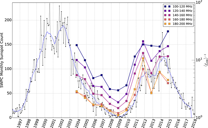
Figure 14. Illustration of how the ionospheric attenuation in our simulations follows the solar cycle by overlaying sunspot number data with the inverse of the expected attenuation factors obtained in our sky model variance simulations. Note the two different vertical axes on the left and right. The thin blue and thin black curves show the historical monthly sunspot numbers from the NOAA Space Weather Prediction Center (https://www.swpc.noaa.gov/products/solar-cycle-progression) over solar cycles 23 and 24. The black points show the count for each month, while the blue curve is a smoothed version of the data obtained by averaging the counts over 13 months. Overlaid are the inverses of the mean over sky realizations of the power spectrum attenuation for each band obtained in the sky model variance simulations at N = 100, i.e., the last point on the curves in Figures 11–13.
Download figure:
Standard image High-resolution imageIt turns out that the years 2011–2014 approximately span the peak of the current solar cycle 24. In contrast, the year 2008—the year of the previous solar minimum—exhibits little or no attenuation even after 100 days. The HERA array should reach its full complement of antennas and observe for 3 yr from 2021 to 2023. Thus, we expect that the next few seasons will pass through solar minimum and be near solar maximum by the end of data taking.
4.4. Fluctuating Polarized Power in the Vokes Parameters
The fluctuation of the ionospheric Faraday rotation turns the otherwise constant (for each t) polarization leakage term into something resembling a stochastic noise term, which is suppressed similarly to the thermal noise by averaging over multiple days of observation. However, unlike the thermal noise, we should not expect the Faraday-rotated polarization to be optimally suppressed by averaging over all the available visibility samples.
For example, this is obvious in the attenuation curve for the year 2012 in Figure 10, where there is a significant lack of monotonicity in the attenuation curves. In this case, if one had visibilities for only the first 40 days, the optimal attenuation is not obtained by averaging over all 40 days; more attenuation could be obtained by only including the first ∼20 days in the average, i.e., by using only half the available data. The reason for this can be observed in Figure 5, where the value of the RM for the year 2012 between days 20 and 40 can be seen to have a corresponding trend reversal, resulting in more coherent averaging of the polarization leakage over this range of days and thus less attenuation. On the other hand, because of the linear trend over tens of days, it is reasonable to expect that an average over a set of days with more separation between them will produce a greater attenuation, since the difference between each day’s RM tends to increase with the number of intervening days.
Given the set of indices of consecutive sidereal days

it is then likely that there are subsets  of nonconsecutive days that will produce significantly more attenuation of the polarization terms in the Vokes parameters than the natural attenuation produced by summing over all consecutive days. There will equivalently be subsets that produce significantly less attenuation or even amplification of the polarization terms.
Figure 15 shows some distributions of  obtained from the fiducial visibility simulations over a collection
  of
of  subsets of S for which the natural attenuation is shown in Figure 10. The number of elements N in each subset Sk is held fixed at N = 50—that is, the elements of each Sk are drawn from S without replacement.
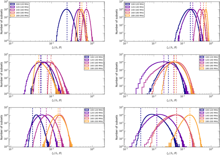
Figure 15. Left: distributions of  . Right: distributions of
  . The distributions are obtained by taking 106 random subsets Sk each of length N = 50 days (i.e., elements of Sk are drawn without replacement) from the fiducial HERA simulations in the years 2009 (top), 2011 (middle), and 2014 (bottom). The dashed lines indicate the 100-day natural attenuation value (i.e., Sk = S, N = 100) of ξI or ξL, not the mean of the distribution. Note the difference in range on the horizontal axes between the left and right panels.
Download figure:
Standard image High-resolution imageThe existence of these wide distributions of attenuation factors suggests a null test that is particularly sensitive to polarization leakage in the delay spectrum estimator of the EOR power spectrum. If the thermal noise is sufficiently suppressed for a given subset size N, then the fluctuation of any problematic polarization leakage should dominate the variation of the different power spectrum estimates. Since variation in the ionospheric Faraday rotation of polarization leakage implies that there will be a distribution of delay power spectra similar to those in Figure 15, the absence of such a distribution rules out polarization leakage as the source of a detection above the expected thermal noise. The converse is not necessarily true—there may be other sources of contamination that could also produce such a distribution, so the presence of such a distribution does not imply that the excess power is due to polarization on the sky.
The best-case scenario is that the magnitude of any polarization leakage is below the cosmological signal level. In this case the effect of ionospheric fluctuations would never be observed directly in the Vokes I spectrum. Therefore, as a consistency check we will want to simultaneously observe the ionospheric fluctuation of the Vokes Q and U parameters. Observing fluctuating polarized power in the Vokes Q/U parameters will then show that there is a fluctuation that would have been observed in Vokes I if the magnitude of polarization leakage had been large enough.
While considering the delay spectra of  and
and  individually can be useful for assessing instrumental systematics (Kohn et al. 2016), we can continue to proceed by analogy to the Stokes parameters to define a quantity analogous to L2 = Q2 + U2 that is maximally sensitive to the magnitude of linear polarization on the sky:

For real data this will include a bias due to Stokes I and the instrumental polarization impurity that is unaffected by the changing Faraday rotations (see Equation 44(b)), and at low frequencies, where the polarization fraction on the sky is small, Stokes I will be at least even with Stokes Q/U in contribution to Vokes Q/U. For the purpose of assessing the attenuation of observed polarized power in our simulation, we follow the same approach here as was applied to Vokes I leakage and subtract the Stokes I term from Vokes Q and Vokes U to isolate the terms that are sensitive to the ionospheric Faraday rotation.
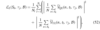
We then define a Vokes polarization delay power spectrum
and thus the relative attenuation factor for the Vokes polarization power

Examples of ξL as computed from our simulations are also shown in Figure 15—the ξL distributions are generated from the exact same collection of subsets Sk that was used for the ξI distributions. We can see that the peaks in the distributions over  and the N = 100 values of ξL (dashed vertical lines in the plots) are comparable to the same quantities for ξI, but they are not perfectly correlated. It is notable that the variance of the ξL distributions is significantly larger than those of ξI, because the definitions of ξI and ξL already divide out an absolute magnitude. Note that this increased variance is not symmetric relative to the peaks of the ξI distributions—the distributions of ξL are relatively skewed toward smaller values. It appears that it is easier to find a combination of Faraday rotations that can significantly attenuate the Vokes polarization power spectrum than it is for the Vokes I polarization leakage.
Another potential issue with this null test is the computational cost in sampling the collection of possible subsets. The number of possible subsets Sk of any length is  , which is ∼1030 for Nd = 100, while the number of subsets of size N = 50 is
  . It is thus not possible to construct the full distributions over all possible subsets even in simulation, much less for actual measurements, which generally require more processing to produce power spectrum estimates. In reality, the number of samples Ns that can be used may only be in the hundreds or thousands.
The distributions in Figure 15 were generated by uniformly sampling the full collection of subsets of length 50. But we are not ignorant of the ionosphere’s behavior, and we would like to be able to use this knowledge to bias the sampling toward the tails of these distributions.
In principle, we might like to use simulations such as the ones done in this paper to inform a selection of subsets with which to estimate the power spectrum. But we have already seen how sensitive the attenuation is to the detailed coupling of the polarization states of the sky to the instrumental response, which casts doubt on our ability to make accurate predictions from simulations given our current levels of knowledge about the relevant functions. Fortunately, for the purpose of this null test we do not need perfect accuracy, only to do a little better than completely random guessing. Additionally, we need not precisely predict the actual magnitude of the attenuation in a particular subset, only its relative place in the distribution.
We attempt to approximate the distribution of  in our fiducial HERA simulations by a simpler functional of the ionospheric RM that is independent of the observed sky and includes only an approximate and generic model of the instrumental response. Define
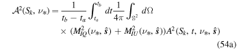

where ν* is the central frequency of each sub-band  , the function A2 is given by Equation (42), and the sums are computed over an nside = 8 HEALPix map, as the integrand does not vary as much on small scales as the functions in our visibility calculation. The Mueller matrix elements used are those of the analytically defined Airy dipole model, computed from the definition of this Jones matrix (Equation (32)) and the formula for the Mueller matrix elements (Equation (20)).
This quantity need not predict the value of the attenuation precisely. We are only interested here in finding subsets that correspond to attenuation factors in the tails of the distributions of ξI in Figure 15. Thus, to compare the distributions for ξI, ξL, and  , we compute the z-scores for each variable from the distribution over the chosen collection
  of subsets Sk. The z-score for the variable
  ,
,  ,
,  is
is

where Mean() and Std() are the mean and standard deviation of X over  , respectively. We denote the z-scores for each of these variables by
  ,
,  ,
,  , respectively.
Figure 16 shows the correlation of  with
with  in the same years and for the same collection of subsets as used in Figure 15. We can see that the subsets that produce values of
  in the tails of the distribution tend to also find values of ξI in the tails of the distribution. The correlation is far from perfect, but as noted, the point is merely to improve the statistical power of the null test—any correlation helps compared to completely uniform sampling. Figure 17 then shows how
  and the cuts on
  are correlated with
  . Additionally, the proxy function
  is simply an inspired guess based on Equation 44(b). It seems likely that an improved method of sampling these distributions based on the ionospheric RM data could be found; in particular, we have not used the fact that the RM has a significant trend as a function of n.
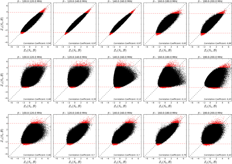
Figure 16. Correlation of the ionospheric fluctuation tracer  with the Vokes I polarization leakage in the fiducial visibility simulation for the years 2009 (top), 2011 (middle), and 2014 (bottom). The collection of 106 subsets used here is the same as the one used to make Figure 15. The red points show a cut on the 500 largest and smallest values of
  for each
  . Such a cut would select the subsets to be used to estimate the power spectrum in our null test.
Download figure:
Standard image High-resolution image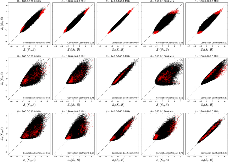
Figure 17. Correlation of the ionospheric fluctuations in the Vokes polarization band power with the Vokes I polarization leakage band power from the fiducial HERA visibility simulations for the years 2009 (top), 2011 (middle), and 2014 (bottom). The red points here correspond to the subsets from the cut on  , i.e., the red points in Figure 16. This shows that if we see a distribution in the Vokes polarization, we can infer that there exists a distribution in the Vokes I polarization, though we should not necessarily expect to see the same distribution.
Download figure:
Standard image High-resolution image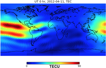
Figure 18. Example output from radionopy: the full-sky TEC content of the ionosphere (in TECU; factors of 1016 electrons per m2) on a Healpix grid, in this case projected onto a python Basemap. This particular snapshot shows the ionosphere at UT 0 hr on 2012 April 11.
Download figure:
Standard image High-resolution image5. Discussion and Conclusions
- 1.Ionospheric attenuation cannot be counted on to suppress polarization leakage in the power spectrum. Given what little is known about the level of polarized power on the sky in the 100–200 MHz frequency band, even at solar maximum it seems as likely as not that this attenuation might suppress polarization leakage to a negligible level. This increases the importance of precise modeling of this systematic, either to show that it will indeed be small relative to the EOR signal, or for the purpose of subtraction.
- 2.Our simulations suggest a definitive test for polarization leakage in the power spectrum. This test comprises the following:
- (a)From the set S of Nd available sidereal days select a collection of subsets with the number N < Nd of elements in each Sk held fixed. The number Nd must be large enough to allow significant ionospheric variation over S. Additionally, the fraction N/Nd must be chosen to strike a balance between allowing the ionospheric attenuation to vary significantly between subsets and also ensuring that each subset represents sufficient integration time on the thermal noise.
- (b)Compute the power spectra PI(Sk) and PL(Sk) for each of the subsets. This produces a distribution of power spectra over.
- (c)If the Vokes I power spectrum estimator is dominated by Stokes I on the sky, then the changing ionospheric Faraday rotations between different subsets will have no effect and each subset will produce the same spectrum up to an expected distribution owing to the thermal noise.
- (d)The distribution of PL should be significantly and obviously inconsistent with the expected thermal noise distribution.
- (e)The null test is passed when both 2(c) and (d) are satisfied, as 2(d) demonstrates that the effective polarized power on the sky has an observable variation over, while 2(c) shows that there is no corresponding variation of what is supposed to be Stokes I.
should be chosen remains open to further investigation. We have shown that a simple proxy function for ionospheric attenuation can reliably bias the sampling toward subsets with relatively high or low attenuation factors. Additional consideration could produce an improved method. The sensitivity of this test as a function of the thermal noise level is explored in a schematic way in Appendix C, but detailed consideration should be the subject of further simulations and analysis that can explore in detail the parameter space of cosmological signal level, thermal noise level, and polarized foreground power level. Additionally, the method of quantifying the consistency of these distributions with an expected thermal noise distribution need not be limited to simply computing the variance. For example, we showed that using our simple proxy function to select subsets can often produce distinctly bimodal distributions. The difference in the means of the high-attenuation collection and the low-attenuation collection could be a useful discriminating statistic. More generally, an advanced subset selection method may go hand in hand with a more robust way of distinguishing the resulting distributions from the expected thermal noise. - 3.The simulations we have used of the polarized sky are intended to be reasonably accurate representations of the expected sky, but their fidelity could certainly be improved. This is necessary for accurate prediction, since we have shown that the level of leakage is sensitively dependent on the correlated structure in the sky model and its alignment with the polarized antenna response, and this does produce large variations in the potential level of leakage. Given this uncertainty, we have purposely avoided considerations of the details of the absolute level of polarization leakage by considering ratios, and we demonstrate that these do show systematic trends independent of the details of the sky model.
- 4.Averaging over sidereal days at fixed LST may still be a useful method for suppressing polarized foregrounds even in the situation in which one tries to model and subtract them directly from the visibilities, as the residual (unmodeled) polarization leakage will be attenuated by averaging over many days. This may ease the requirements on the completeness of the polarized model. On the other hand, an increasing level of ionospheric attenuation goes hand in hand with increasing complexity of the ionosphere, and thus increasing complexity of the model that must be constructed in order to perform the subtraction. It remains to be seen whether the global model of the ionospheric Faraday rotation that we have presented here would be adequate for such a task.
- 5.The variance in the visibility and resulting power spectrum can be quite large when the polarization angle on the sky is not constrained. While preliminary, the results of our simulations suggest that a statistical foreground model that does not constrain the orientation of the polarization on the sky may be inadequate for predicting polarization leakage levels to the accuracy required for HERA, and possibly other EOR experiments. Determining the extent to which this is true or not through more careful consideration of the parameterization of the sky model and the mapping into the visibility will require further research. Obviously, it is necessary to determine the polarization angle accurately to be able to subtract a model from the visibilities.


This material is based on work supported by the National Science Foundation under grant nos. 1440343 and 1636646, the Gordon and Betty Moore Foundation, and institutional support from the HERA collaboration partners. S.A.K. is supported by a University of Pennsylvania SAS Dissertation Completion Fellowship. J.E.A. acknowledges support from NSF CAREER award no. 1455151.
Appendix A: Comparing Ionospheric RM Outputs
There are now several software packages that interpret CODE ionex files specifically for the use of low-frequency radio interferometers. Two of these are ionFR (Sotomayor-Beltran et al. 2013) and the results shown in Arora et al. (2015). In Figure 19 we show qualitative agreement with both of these works by comparing maps of vertical TEC values over the globe. In Figure 20 we show radionopy and ionFR RM output for a single pointing toward Cassiopeia A (Cas A; R.A. = 23h23m279, decl. = +58°48′42
4) from the LOFAR Core site in the Netherlands, which exhibit quantitative agreement. Slight offsets at the highest RM values that day can be attributed to differences in our interpolation schemes.
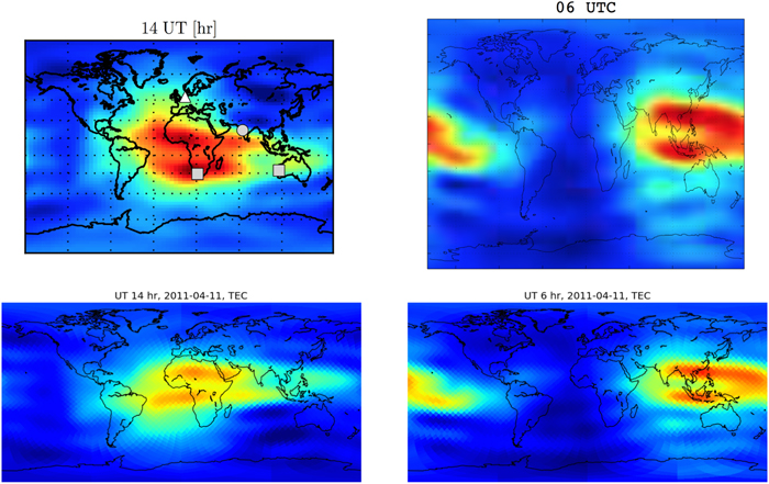
Figure 19. Top: vertical TEC from the CODE ionex file for 2011 April 11, overplotted on the globe in a Cartesian projection, as measured in Sotomayor-Beltran et al. (2013) and Arora et al. (2015) (left and right, respectively). Bottom: radionopy output for the same times and day. There is qualitative agreement, save for an error resulting in upside-down maps in Sotomayor-Beltran et al. (2013), as pointed-out by Arora et al. (2015).
Download figure:
Standard image High-resolution image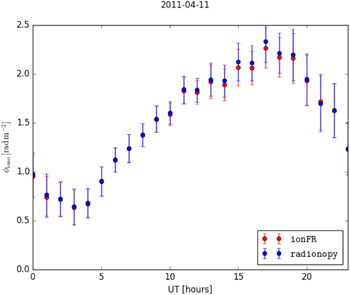
Figure 20. RM of Cas A as viewed from the LOFAR Core site in the Netherlands on 2011 April 11, according to ionFR and radionopy. The two codes show quantitative agreement; this demonstrates that radionopy can be used for single-pointing as well as full-sky RM measurements.
Download figure:
Standard image High-resolution imageAppendix B: The Instrumental Jones Matrix and Basis Transformation
While the instrumental Jones matrix  happens to be a 2 × 2 matrix in the case of the antenna with two different feed polarizations, it is better thought of as a list of rank-1 tensor fields
  for the kth feed of N feeds

that correspond to the far-field electric vector fields generated by each feed operated in transmission. Each row of the matrix corresponds to the normalized electric vector field pattern of a single feed of the antenna.
In order to compute Equation 12(a), the instrumental Jones matrix  and the coherency matrix
  must be specified in the same basis. Because of the cylindrical symmetry of the
  ,
,  basis, we can specify the instrumental response in this basis, rather than the alternative of performing a basis transformation on the observed coherency matrix. Observe that the integrand in Equation 12(a) is invariant under a transformation


where  is a 2 × 2 unitary matrix field. Any basis transformation (a point-by-point 2 × 2 rotation) is such a unitary matrix. Since the coherency matrix is specified in the
  basis, we thus require the instrumental response to be specified in this basis.
However, it is generally practical to specify the instrumental response in a basis of spherical coordinates local to the antenna so that the representation is independent of the telescope’s geographic location, and a standard choice of coordinates is the zenith angle θ ∈ (0, π) and local azimuthal angle  . Explicitly, this means that the electric field data generated from an EM simulation of the antenna are specified as the complex coefficient functions of the vector field

which defines the instrumental response as


where  denotes the direction of the antenna’s boresight. There is an equivalent representation of this vector field
  in the equatorial basis

The components in the two different bases are related by




which defines a rotation matrix field  with elements


For two feeds a and b with the response of each given by the vector fields  and
and  , the instrumental Jones matrix is then specified in the equatorial basis as

Appendix C: Effect of Thermal Noise in Polarization Null Test
Since we have not included the effect of thermal noise or an absolute scale for the polarized power in our analysis, we consider a schematic model of how these variables would affect the statistics of the proposed null test. The point is to argue that if polarization leakage were the limiting systematic in the power spectrum, the variance in our null test due to fluctuations in the polarized power will eventually dominate the variance due to thermal noise.
Let  be the Stokes I contribution to the power spectrum,
  the contribution of Stokes Q and U, and
  the thermal noise with mean
  ; for simplicity of exposition we neglect cross-terms between Stokes parameters. The power spectrum

can then be considered a random variable over the collection  of subsets of sidereal days, as each subset produces a different realization of the noise, and changing ionospheric attenuation produces a fluctuation in
  . The
. The  term, which represents the cosmological signal, is taken to be constant over the subsets. If
  is the intrinsic polarized power, then the attenuation factor is


where  is defined by the mean of
  over
over  ,
,

The polarized power can also be written as


so we can see that

The mean and variance of  are then




If  , then we detect the cosmological signal with an uncertainty dominated by the thermal noise and any other small systematics. If
  , then we can see that the ionospheric fluctuation of
  in our null test will dominate the variance due to thermal noise—we will have been thwarted from observing cosmological reionization, but we will not be fooled into thinking otherwise.
In a regime where polarization leakage is comparable to the cosmological signal, we would have  , and thus the second term is approximately the thermal-noise-to-signal ratio on a detection in the absence of
  . The HERA experiment is designed to detect the EOR power spectrum at high signal-to-thermal-noise ratio, so even in a regime where
  is slightly smaller than
  the excess variance in the null test should still be detectable.
Footnotes
- 1
- 2
https://github.com/UPennEoR/IonRIME. Note that this is intended only to provide documentation for the results, as the code does not constitute a user-friendly software package.
- 3
- 4
- 5