Abstract
We use continuous wavelet transform techniques to construct the global and environment-dependent wavelet statistics, such as energy spectrum and kurtosis, to study the fluctuation and intermittency of the turbulent motion in the cosmic fluid velocity field with the IllustrisTNG simulation data. We find that the peak scale of the energy spectrum defines a characteristic scale, which can be regarded as the integral scale of turbulence, and the Nyquist wavenumber can be regarded as the dissipation scale. With these two characteristic scales, the energy spectrum can be divided into the energy-containing range, the inertial range, and the dissipation range of turbulence. The wavelet kurtosis is an increasing function of the wavenumber k, which first grows rapidly then slowly with k, indicating that the cosmic fluid becomes increasingly intermittent with k. In the energy-containing range, the energy spectrum increases significantly from z = 2 to 1, but remains almost unchanged from z = 1 to 0. We find that both the environment-dependent spectrum and kurtosis are similar to the global ones, and the magnitude of the spectrum is smallest in the lowest-density and largest in the highest-density environment, suggesting that the cosmic fluid is more turbulent in a high-density than in a low-density environment. In the inertial range, the energy spectrum’s exponent is steeper than both the Kolmogorov and Burgers exponents, indicating more efficient energy transfer compared to Kolmogorov or Burgers turbulence.
Original content from this work may be used under the terms of the Creative Commons Attribution 4.0 licence. Any further distribution of this work must maintain attribution to the author(s) and the title of the work, journal citation and DOI.
1. Introduction
The turbulent motion of the cosmic baryonic fluid in large-scale structures of the universe has attracted increasing attention in cosmological studies over the last several decades. The physical origin of turbulence in cosmic baryonic fluids is complex and diverse, mainly including the following. Accretion through structure formation or hierarchical mergers should be able to generate and sustain turbulence in the intergalactic medium (IGM) and in galaxy clusters (K. Subramanian et al. 2006; A. Bauer & V. Springel 2012; L. Iapichino et al. 2017), and the associated physical processes, such as the injection and amplification of vorticity by shock waves (e.g., D. Ryu et al. 2008; D. H. Porter et al. 2015; F. Vazza et al. 2017) or ram pressure stripping (e.g., R. Cassano & G. Brunetti 2005; K. Subramanian et al. 2006; E. Roediger & M. Brüggen 2007), can also generate turbulence in clusters of galaxies. In addition, outflows or feedbacks from active galactic nucleus (AGN) jets, which inflate buoyant bubbles and eventually stir the intracluster medium (ICM), are expected to drive turbulence and heat cluster cores (M. Brüggen et al. 2005; L. Iapichino & J. C. Niemeyer 2008; M. Gaspari et al. 2011; N. Banerjee & P. Sharma 2014; M. Angelinelli et al. 2020), and the supernova (SN)-driven galactic winds are also expected to generate turbulence in and around galaxies (e.g., C. Evoli & A. Ferrara 2011; L. Iapichino et al. 2013).
Observational evidence for turbulent motions in the ICM has been provided by direct detection of nonthermal broadening of the X-ray emission lines by the Hitomi satellite (Hitomi Collaboration et al. 2016), and by indirect observations such as fluctuations in the magnetic field in the diffuse cluster radio sources (C. Vogt & T. A. Enßlin 2003; M. Murgia et al. 2004; C. Vogt & T. A. Enßlin 2005; T. A. Enßlin & C. Vogt 2006; A. Bonafede et al. 2010; V. Vacca et al. 2010, 2012), fluctuations in the X-ray surface brightness or in pressure inferred from X-ray and Sunyaev–Zel’dovich effect maps (P. Schuecker et al. 2004; E. Churazov et al. 2012; I. Zhuravleva et al. 2014; M. Gaspari et al. 2014; S. A. Walker et al. 2015; R. Khatri & M. Gaspari 2016; I. Zhuravleva et al. 2018), and the suppression of resonant line scattering in the X-ray spectra (E. Churazov et al. 2004; I. Zhuravleva et al. 2013; Hitomi Collaboration et al. 2018; X. Shi & C. Zhang 2019). These effects can be used to detect and measure turbulence in the cosmic baryonic fluids. In addition to observations, the origin and evolution of turbulence in cosmic baryonic matter has been extensively studied using various cosmological hydrodynamical simulations (e.g., M. L. Norman & G. L. Bryan 1999; K. Dolag et al. 2005; L. Iapichino & J. C. Niemeyer 2008; E. T. Lau et al. 2009; W. Zhu et al. 2010; F. Vazza et al. 2011; F. Miniati 2014; M. Gaspari et al. 2014; M. Brüggen & F. Vazza 2015; M. Angelinelli et al. 2020).
There are a large number of problems relevant to the study of the formation and evolution of galaxies and galaxy clusters. Among these, the study of the heating mechanisms in the ICM and IGM is particularly important. If there is no sufficient heating mechanism, then there will be a phenomenon called cooling flow within the galaxy clusters, and there will also be an excess of star birth in the galaxy, which is known as the overcooling problem (G. M. Voit 2005). In addition, a heating mechanism may also be responsible for the missing baryon problem (J. N. Bregman 2007).
The main proposals to overcome this overcooling problem are the heating mechanisms, such as SN or AGN feedback, and turbulence in the IGM or ICM. In the popular semianalytical models of galaxy formation, the heating mechanism is mainly based on SN and AGN feedback, and turbulent heating is not considered (Q. Guo et al. 2011; B. M. B. Henriques et al. 2015). However, some studies suggest that turbulent heating has a significant effect and should not be ignored. For example, W. Zhu et al. (2010) suggests that the turbulent pressure can be compared to the thermodynamic pressure of the baryonic gas. Furthermore, I. Zhuravleva et al. (2014) suggests that turbulent heating is sufficient to offset radiative cooling, and indeed appears to be locally balanced at each radius, which may be a key element in solving the gas cooling problem in cluster cores.
In a series of papers, we have carried out a number of studies on the turbulence of the cosmic baryon fluid, briefly summarized as follows. B. Kim et al. (2005) explore the dynamics and evolution of the baryonic gas in the universe, focusing on its velocity field and its interaction with the dark matter gravity, and discuss the implications of a Burgers fluid model for describing the dynamics of the IGM, highlighting the importance of considering heating and cooling processes in understanding the evolution of the IGM. Using the WIGEON hydrodynamical simulation (L.-L. Feng et al. 2004), P. He et al. (2006) shows that the intermittency of the velocity field of the cosmic baryonic fluid at redshift z = 0 in the scale range from the Jeans length, roughly 0.1–0.3 h−1 Mpc, to about 16 h−1 Mpc can be described extremely well by She–Leveque's universal scaling formula, and these results imply that the motion of the highly evolved cosmic baryonic fluid is similar to a fully developed turbulence. H.-Y. Yang et al. (2020) use updated WIGEON data (W. Zhu et al. 2013) and study the turbulence-induced deviation of the spatial distributions between baryons and dark matter. They find that at z = 0, at the 1% deviation level, the deviation scale is about 3.7 h−1 Mpc for the density field, while it is as large as 23 h−1 Mpc for the velocity field, a scale that falls into the weakly nonlinear regime of the density field for the structure formation paradigm. Their results also suggest that the effect of turbulence heating is comparable to that of these processes such as SN and AGN feedback. H.-Y. Yang et al. (2022) compare the results derived from IllustrisTNG and WIGEON simulations, and find that for the ratio of the density power spectrum between dark matter and baryonic matter, as scales become smaller and smaller, the power spectra for baryons are increasingly suppressed for WIGEON simulations, while for TNG simulations, the suppression stops at k = 15–20 h Mpc−1, and the power spectrum ratios increase when k > 20 h Mpc−1. These results indicate that turbulent effects can also have the consequence of suppressing the power ratio between baryons and dark matter. These are of great importance for understanding the distribution and evolution of baryonic matter in the universe, as well as issues related to galaxy formation, and therefore turbulence in the cosmic baryonic fluid is worthy of in-depth study.
The wavelet analysis technique is a powerful tool, and the application of the wavelet transform technique to turbulence can be traced back more than three decades. In a review article, M. Farge (1992) extensively discusses wavelet transforms as a powerful tool for achieving scale localization, allowing for the analysis of different scales of motion in turbulent flows. This article delves into the computation of local energy spectra, wavelet coefficients, and statistical properties, showing how wavelet analysis facilitates the investigation of coherent structures, intermittency, and other key aspects of turbulence. It also details the application of wavelet transforms to turbulence analysis, emphasizing their ability to provide a localized and multiscale view of the flow, leading to insights into coherent structures, intermittency, and statistical properties. M. Farge (1992) emphasizes the advantages of wavelet analysis over traditional methods and provides concrete examples of its application to turbulent phenomena, providing a valuable resource for fluid mechanics researchers seeking a multiscale perspective on turbulent flows.
The wavelet analysis method can also find its application in the study of cosmological turbulence. To name just a few that are relevant to our current interests. P. Schuecker et al. (2004) construct two-dimensional (2D) pressure maps from XMM-Newton observations of the Coma galaxy cluster using wavelet methods, which effectively suppress noise and reveal small-scale turbulence structures, helping to isolate and analyze pressure fluctuations, enabling the computation of their power spectra and providing evidence for turbulence in the ICM. G. Kowal & A. Lazarian (2010) use wavelet analysis to decompose the velocity field of compressible magnetohydrodynamic turbulence into Alvén, slow, and fast modes, and investigate in detail the turbulence properties such as spectra, anisotropy, scaling exponents and intermittency, showing that these properties are influenced by both the sonic and Alvén Mach numbers. X. Shi et al. (2018) use a novel wavelet analysis method to study the radial dependence of the ICM turbulence spectrum, and find that faster turbulence dissipation in the inner high-density regions causes the turbulence amplitude to increase with radius. They also find that the ICM turbulence at all radii decays in two phases after a major merger, i.e., an early fast-decay phase and a slow secular-decay phase.
In a series of works, we have used the continuous wavelet transform (CWT) to construct the wavelet statistics, such as the wavelet power spectrum (WPS), wavelet cross-correlation and wavelet bicoherence, as well as the environment-dependent WPS (env-WPS), and analyzed the clustering and non-Gaussian properties of large-scale structures in the universe using the cosmological simulation data (Y. Wang & P. He 2021, 2022; Y. Wang et al. 2022). In a recent paper (Y. Wang & P. He 2024), we mainly use the env-WPS to study how baryonic effects vary with scale and local density environment. In addition, we also complete a comparative study of several fast algorithms for one-dimensional (1D) CWT (Y. Wang & P. He 2023).
In this work, we apply the CWT techniques to the IllustrisTNG simulation data to study the turbulent motion of the cosmic baryonic fluid in the large-scale structures of the universe. This paper is organized as follows. In Section 2, we briefly introduce our methods and the simulation data used in this work. In Section 3, we present the results of our work. In Section 4, we present the summary and conclusions of the paper.
2. Methods and Data
2.1. Continuous Wavelet Transform and Power Spectrum
For a random field with the zero mean value, say the three-dimensional (3D) velocity field of the cosmic baryonic fluid
u
, its isotropic CWT  is obtained by convolution with the wavelet function Ψ as

Throughout this work, we use the so-called 3D isotropic cosine-weighted Gaussian-derived wavelet (CW-GDW), which can achieve good localization in both spatial and frequency space simultaneously (Y. Wang & P. He 2022, 2024). It is defined in real space as
with its Fourier transform
where r = ∣
x
∣, k = ∣
k
∣, and  is the normalization constant such that ∫∣Ψ(
x
)∣2
d3
x
= 1.
is the normalization constant such that ∫∣Ψ(
x
)∣2
d3
x
= 1.
In many cases, we compare the results of the CWT with those of the Fourier transform, such as comparing the global WPS with the Fourier power spectrum (FPS). However, the wavelet scale w and the Fourier wavenumber k are not simply equal, but have a correspondence w = cw k, where cw ≃ 0.3883 for the 3D isotropic CW-GDW (see Appendix A).
With the CWT  , we can define the env-WPS of the velocity field as
where the environment is specified with the dark matter density contrast  . For the environment Δ, we specify a density interval δ1 < Δ < δ2 as the density-limiting condition, and determine all the spatial regions V1, V2, V3, ..., with VΔ = V1 ∪ V2 ∪ V3..., such that the density-limiting condition is satisfied within VΔ. The spatial coordinate
x
runs over all the spatial region VΔ, and we count the number of all the coordinates as NV
. In this way, we obtain the env-WPS of Equation (4). If the density interval is taken as 0 < Δ < ∞ , then we obtain the global WPS as,
. For the environment Δ, we specify a density interval δ1 < Δ < δ2 as the density-limiting condition, and determine all the spatial regions V1, V2, V3, ..., with VΔ = V1 ∪ V2 ∪ V3..., such that the density-limiting condition is satisfied within VΔ. The spatial coordinate
x
runs over all the spatial region VΔ, and we count the number of all the coordinates as NV
. In this way, we obtain the env-WPS of Equation (4). If the density interval is taken as 0 < Δ < ∞ , then we obtain the global WPS as,

which is actually calculated by averaging over all spatial positions. It can be seen that the global WPS  is related to the FPS P
u
(k) as (Y. Wang et al. 2022)
is related to the FPS P
u
(k) as (Y. Wang et al. 2022)

One can see that the global WPS is the wavelet-weighted average of the FPS in k space. The former therefore has a similar but smoother shape to the latter. Obviously, the wider the bandwidth of the wavelet function, the smoother the global WPS. If the bandwidth is narrower, the global WPS is closer to the FPS.
Integrating both sides of Equation (6) with respect to w, we can obtain an approximate relationship with the correspondence w = cw k as

where  is a constant depending on the wavelet function. Therefore, the global WPS and the FPS differ by only a scaling factor that depends on the specific wavelet function selected. Obviously, for the power-law power spectrum P
u
(k) ∝ kn
,
is a constant depending on the wavelet function. Therefore, the global WPS and the FPS differ by only a scaling factor that depends on the specific wavelet function selected. Obviously, for the power-law power spectrum P
u
(k) ∝ kn
,  preserves the same power index. For the 3D isotropic CW-GDW used in this work, IΨ/(2π2
cw
) ≈ 1.0754, at which point the shape and size of the global WPS and FPS are very close (see Appendix A). However, due to the simultaneous spatial and frequency localization of the CWT, we can specify any shape of the region for integration, such as a density-bounded region. Therefore, we can define the env-WPS as in Equation (4). Because the env-WPS can be calculated in spaces of arbitrary shapes, whereas the FPS is only restricted to regular shapes such as squares or cubes, the techniques of wavelet analysis are superior to those of Fourier analysis, as demonstrated in Figure 1.
preserves the same power index. For the 3D isotropic CW-GDW used in this work, IΨ/(2π2
cw
) ≈ 1.0754, at which point the shape and size of the global WPS and FPS are very close (see Appendix A). However, due to the simultaneous spatial and frequency localization of the CWT, we can specify any shape of the region for integration, such as a density-bounded region. Therefore, we can define the env-WPS as in Equation (4). Because the env-WPS can be calculated in spaces of arbitrary shapes, whereas the FPS is only restricted to regular shapes such as squares or cubes, the techniques of wavelet analysis are superior to those of Fourier analysis, as demonstrated in Figure 1.
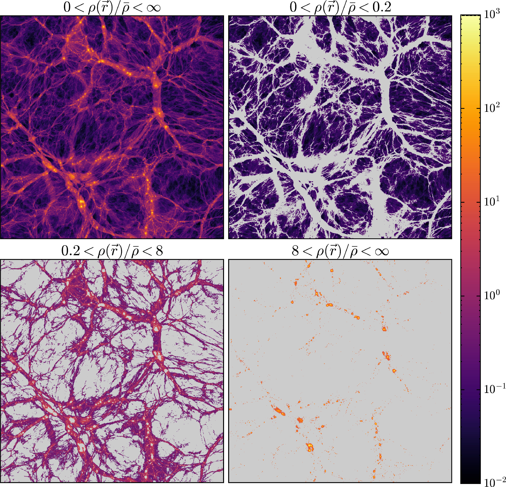
Figure 1. A 2D slice of the IllustrisTNG100-1 dark matter density field at z = 0 (top left-hand panel), and spatial regions corresponding to the density ranges labeled in these panels. The slice covers a 75 × 75h−2 Mpc2 area with a thickness of 0.3 h−1 Mpc. The gray background indicates the region outside the specified density range. Fourier analysis can only be applied to the regular region, such as a square or a cube (top left-hand panel), whereas wavelet analysis can be applied to regions of any shape (all four panels).
Download figure:
Standard image High-resolution imageIncidentally, it is not necessary to use anisotropic wavelets to compute the velocity WPS. In Y. Wang & P. He (2022), we compute the matter WPS using both 3D isotropic and anisotropic wavelet, and find that they yield almost identical results. For details of the CWT techniques that we have developed, please refer to Y. Wang & P. He (2021), Y. Wang et al. (2022), Y. Wang & P. He (2022, 2023), and Y. Wang & P. He (2024).
2.2. Turbulence in the Cosmic Baryonic Fluid
As mentioned in Section 1, the cosmic baryonic fluid is characterized by turbulent motion. In this work, we investigate in which regions, to what extent, and on which scales the cosmic baryonic fluid is turbulent.
2.2.1. Filtering Out the Bulk Flow
Although it is difficult to define turbulence (P. A. Davidson 2015), we can still provide a description of turbulent flow in fluids and distinguish between turbulent and bulk flow.
In general, a velocity field of the fluid u is a superposition of the turbulent velocity and the bulk velocity, i.e., u = u turb + u bulk. Bulk flow is a flow state in which the fluid particles move in a relatively orderly manner, and the flow velocity and direction are relatively uniform in a given cross section. In contrast, turbulent flow refers to a chaotic, disordered flow state in which the fluid particles move irregularly and randomly, and usually occurs when the fluid velocity is high, the pressure gradient is large, or the Reynolds number exceeds a certain critical value. Turbulent flow has the characteristics of rapid mixing, strong diffusion, and good heat transfer. Therefore, it is necessary to develop an approach to separate the turbulent flow from the bulk motion (e.g., D. Vallés-Pérez et al. 2021; K. Dolag et al. 2005; F. Vazza et al. 2012; J. A. ZuHone et al. 2013; X. Shi et al. 2018; M. Angelinelli et al. 2020).
In this study, we utilize the code based on the iterative multiscale filtering approach of F. Vazza et al. (2012, see the Appendix of their paper) to extract turbulent motions from the velocity field of the cosmic fluid. Specifically, we apply no weighting scheme when calculating the local mean velocity field, i.e., wi = 1 in Equation (3) of F. Vazza et al. (2012). To use the code, we set the relevant parameters as eps=0.05, epssk=0.5 and nk=16.
2.2.2. Intermittency of Turbulence
In general, there are two types of turbulence in fluids, Kolmogorov turbulence and Burgers turbulence. Kolmogorov turbulence is essentially excited by subsonic motion of the flow, and characterized by eddies of different scales (A. Bauer & V. Springel 2012). In the fully developed state, the fluid satisfies ∇ ·
u
= 0, and its kinetic energy spectrum follows the Kolmogorov's k−5/3 scaling-law. Burgers turbulence is essentially excited by supersonic motion of the flow (S. Boldyrev et al. 2004; C. Federrath et al. 2010; A. Bauer & V. Springel 2012) and characterized by shock waves (L. Konstandin et al. 2015), which gives k−2 for the kinetic energy spectrum at steady state when  , the Reynolds number, satisfies
  , where Lc is some correlation length (E. Balkovsky et al. 1997). The turbulence in the cosmic baryonic fluid is composed of both Kolmogorov turbulence and Burgers turbulence, but it is not simply a mixture of the two types of turbulence, as will be discussed later.
In turbulence, the presence of shocks leads to a strong intermittency, and therefore the turbulent energy dissipation in space is also intermittent. Intermittency in turbulence refers to the phenomenon where fluctuations in velocity, pressure, or other flow properties occur in a sporadic or irregular manner. Intermittency arises because these fluctuations are not uniformly distributed in space and time. Studying intermittency helps in understanding how energy cascades from large to small scales and dissipates. Usually, the deviation of the tails of the probability density function (PDF) from Gaussian is seen as a manifestation of intermittency, with a highly unusual scaling for the moments of the velocity differences (E. Balkovsky et al. 1997). Therefore, to characterize the intermittency of turbulence in the cosmic fluid, as in C. Meneveau (1991) and J. M. Angulo & A. E. Madrid (2023), we define the wavelet global kurtosis (or flatness) of the cosmic velocity field as

and the wavelet environment-dependent (env-) kurtosis as

in which  is the CWT of the velocity component along a given axis, and
  . For a scalar Gaussian field, the kurtosis = 3, whereas for the turbulent velocity field of fluids, its PDF is generally a long-tailed distribution, with kurtosis > 3.
Kurtosis can be thought of as a measure of the intermittency of the turbulence. The greater the kurtosis, the more intermittent the cosmic flow should be.
Note that M. Farge (1992) use the local wavelet energy spectrum of the velocity field to define the local intermittency of turbulent flow, see their Equation (59). We do not use this definition because we have already used env-WPS to perform the spectral analyses throughout this work.
2.2.3. Ratio of Power Spectra of the Two Modes
The velocity field of the cosmic baryonic fluid u can be separated by the Helmholtz–Hodge decomposition (G. B. Arfken & H. J. Weber 2005) into a compressive (or longitudinal) part “∥” and a solenoidal (or transverse) part “⊥”, as u = u ∥ + u ⊥, where the compressive part u ∥ satisfies ∇ × u ∥ = 0, and the solenoidal part u ⊥ satisfies ∇ · u ⊥ = 0, respectively. In Figure 2, we present a visualization of the velocity field for the TNG50 data at z = 0.
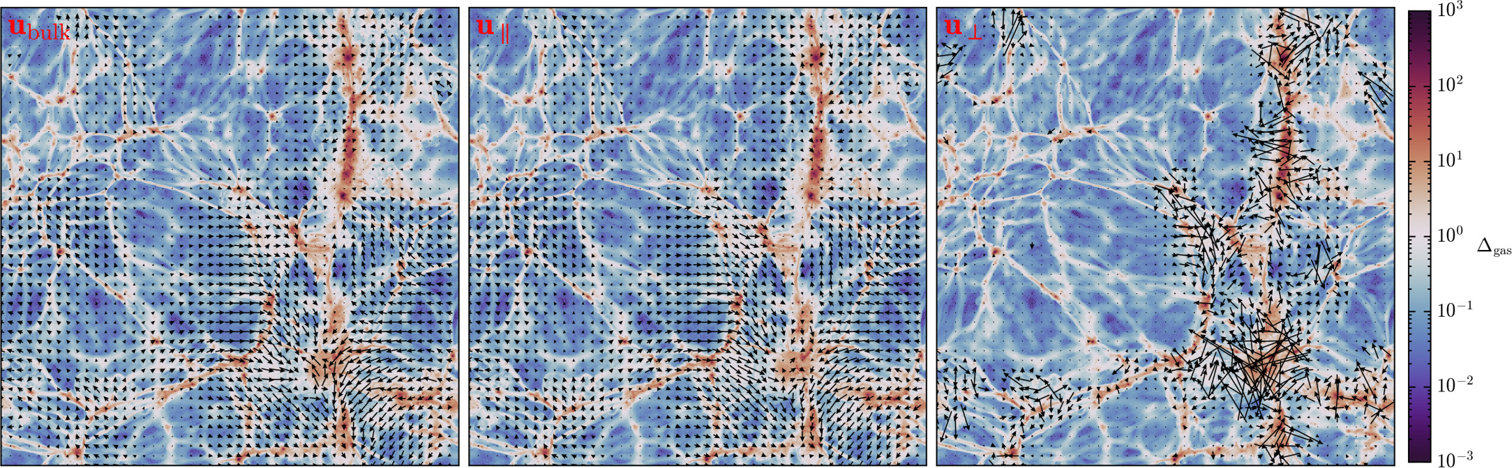
Figure 2. A 2D slice of the velocity field for the TNG50-1 data at z = 0. The slice covers a 35 × 35h−2 Mpc2 area with a thickness of 0.18 h−1 Mpc. The line of sight is along the z-axis, and only the velocity in the x–y direction is displayed. The panels on the left-hand, middle, and right-hand correspond to the bulk velocity
u
bulk, the compressive component
u
∥, and the solenoidal component
u
⊥, respectively. The background represents the density contrast  of the baryonic fluid.
Download figure:
Standard image High-resolution imageFor the divergence d ≡ ∇ · u and the vorticity ω ≡ ∇ × u of the velocity field of u , it is easy to show that

in which Pd (k), Pω (k), P∥(k), and P⊥(k) are the FPS of d, ω , the velocity component u ∥, and u ⊥, respectively.
The small-scale compression ratio can be defined as follows (S. Kida & S. A. Orszag 1990; W. Schmidt et al. 2009)
This ratio quantifies the relative importance of the compressive and solenoidal modes in a flow (L. Iapichino et al. 2011). Inspired by this compression ratio, we define the FPS ratio of the solenoidal mode to the total turbulence as

It can be seen that Q(k) is superior to rCS because it is scale dependent. Similar to the FPS ratio in Equation (12), we can also define the global WPS ratio as

in which  ,
,  ,
,  , and
, and  are global WPS of d,
ω
, the velocity component
u
∥, and
u
⊥, respectively, computed in the same way as Equation (5), and the correspondence w = cw
k is used to convert w to k.
are global WPS of d,
ω
, the velocity component
u
∥, and
u
⊥, respectively, computed in the same way as Equation (5), and the correspondence w = cw
k is used to convert w to k.
As mentioned above, the turbulence in the cosmic fluid consists not only of Kolmogorov turbulence, but also of Burgers turbulence. Therefore, it is not proper to treat the turbulent energy spectrum as consisting only of the solenoidal component (see, D. Ryu et al. 2008), and it is better to take Pd
(k) + Pω
(k), or its wavelet counterpart  , as the total energy spectrum. Thus, Q(k) and
  reflect the solenoidal fraction of the total turbulence energy as a function of k.
With the env-WPS of the velocity field in Equation (4), we can also define the env-WPS ratio as
in which  ,
,  ,
,  , and
, and  are the env-WPS of d,
ω
, the velocity component
u
∥, and
u
⊥, respectively.
are the env-WPS of d,
ω
, the velocity component
u
∥, and
u
⊥, respectively.  is the ratio of the solenoidal component to the total energy as a function of k and the environment δ.
2.3. Simulation Data
We utilize data from the IllustrisTNG simulations (TNG for short) (A. Pillepich et al. 2018b; D. Nelson et al. 2018; F. Marinacci et al. 2018; J. P. Naiman et al. 2018; V. Springel et al. 2018; D. Nelson et al. 2019), focusing on the samples TNG300-1, TNG100-1, and TNG50-1. These samples correspond to simulated universes of sizes 205 h−1 Mpc, 75 h−1 Mpc, and 35 h−1 Mpc, respectively. TNG simulations are comprehensive, encompassing large-scale gravo-magnetohydrodynamical processes within the cosmos, and are executed using the moving-mesh code AREPO (V. Springel 2010). This code employs a second-order accurate Godunov-type scheme for the hydrodynamic equations on a dynamically unstructured mesh, improving the fidelity of both supersonic and subsonic fluid turbulence simulations. A. Bauer & V. Springel (2012) demonstrated AREPO's superiority in accurately replicating turbulence, achieving Kolmogorov-like scaling laws for density, velocity, and vorticity power spectra, aligning with theoretical expectations from the fully developed isotropic turbulence.
In addition to gravitational and hydrodynamic calculations, the TNG simulations incorporate a comprehensive set of physical processes (A. Pillepich et al. 2018a; D. Nelson et al. 2019), which include: (1) the formation and evolution of stars, (2) the associated metal enrichment and loss of mass, (3) cooling processes for primordial and metal-enriched gases, (4) the impact of SN on the pressurization of the interstellar medium, without resolving individual SN events, (5) feedback from stars, manifesting as galactic winds powered either by SN or stars in the asymptotic giant branch (AGB), (6) the formation and growth of supermassive black holes, accompanied by energy feedback from AGN in both high-accretion quasar and low-accretion kinetic wind phases, and (7) the role of magnetic fields in cosmic structures.
Given the abundance of the physical processes included in the TNG simulations and AREPO's excellent performance in hydrodynamical computations, the TNG data are well suited for studying cosmic fluid turbulence.
3. Results
We use the piecewise cubic spline (PCS) scheme (E. Sefusatti et al. 2016) to assign all the simulation particles into a 15363 grid, and with this grid we can use FFT to compute the FPS and WPS (see Y. Wang & P. He 2024 for the numerical pipeline).
3.1. The Global Results
As mentioned in Section 2.2.1, in all the following computations the bulk flow has been removed from the velocity field using the approach of F. Vazza et al. (2012).
In Figure 3, we show both the FPS and the global WPS at z = 0 for the velocity field
u
and its “∥” and “⊥” components of the cosmic fluid, with the corresponding spectral ratios Q(k) and  . From top to bottom are the results for the TNG300, TNG100, and TNG50 simulations, respectively. As analyzed in Section 2.1, the global WPS is almost the same as the FPS, just with a slightly higher factor. The ratios Q(k) and
  also give almost the same results. Indeed, we observe that the Fourier analysis and the global wavelet analysis give consistent results, suggesting that the wavelet analysis is valid.
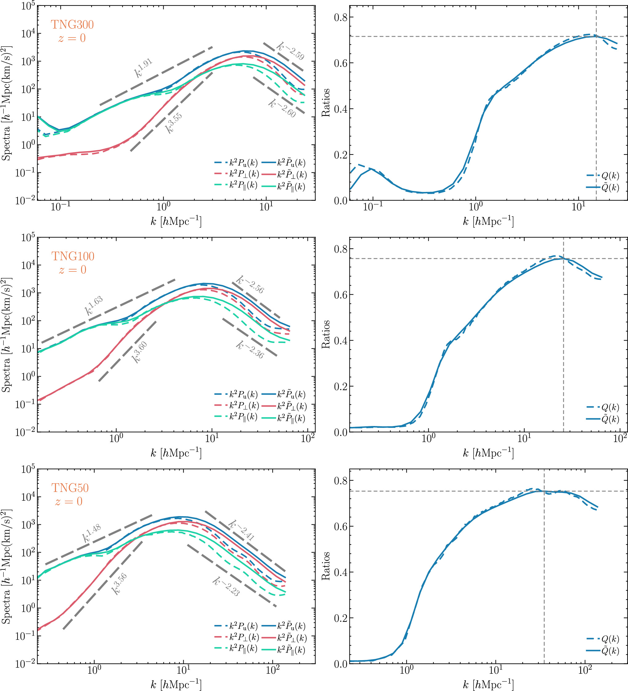
Figure 3. Both Fourier and global wavelet energy spectra at z = 0 for the velocity field u , its “∥” and “⊥” component of the cosmic fluid (left column), with the corresponding spectral ratios (right column). From top to bottom are the TNG300, TNG100, and TNG50 data, respectively. To aid the eye, the relevant power laws are indicated in the figure.
Download figure:
Standard image High-resolution imageIt can be seen that there are peaks in all energy spectra of the velocity
u
of the cosmic fluid, and the peak scales are kS−peak = 6.0, 8.2, and 8.8 h Mpc−1, i.e., the length scale 1.0, 0.76, and 0.71 h−1 Mpc for TNG300, TNG100, and TNG50, respectively. It seems that the peak scales are roughly 1/5 − 1/3 of the sizes of virialized cluster halos. At large scales, i.e., k < kS−peak, the energy spectra are increasing functions of k and the turbulent velocity
u
turb is mostly dominated by its compressive component. Within this scale range, the gravitational collapse converts the potential energy of the structure into kinetic energy of the bulk flow, and the bulk flow further decays into turbulent flows—first in the compressive mode and, with increasing k, mostly in the solenoidal mode, as can also be seen from the spectral ratios Q(k) and  . The transition scales of the two modes can be determined by setting
  or Q(ktrans) = 1/2, and thus we get ktrans = 1.9, 2.9, and 2.7 h Mpc−1 for TNG300, TNG100, and TNG50, respectively.
According to the analysis by W. Zhu et al. (2010), the baroclinic term in their dynamical Equation (1) drives the growth of vorticity over time, which becomes more effective during the nonlinear evolutionary stage. We observe that the WPS of the solenoidal mode increases significantly faster with k compared to that of the compressive mode if k < kS−peak. This is likely the reason for the dips observed at k ∼ 1 h Mpc−1.
One can see that the energy spectra drop rapidly at k > kS−peak. As shown in the figure, the exponent of the energy spectrum within this scale range is −2.59, −2.56, and −2.41 for TNG300, TNG100, and TNG50, respectively, which are all steeper than not only the Kolmogorov exponent −5/3 but also the Burgers turbulence exponent −2. As discussed in Section 2.2.2, Kolmogorov turbulence is excited by subsonic motion of the flow, characterized by eddies of different scales, and hence the u ⊥ component is mostly responsible for Kolmogorov turbulence, while Burgers turbulence is excited by supersonic motion, characterized by shock waves, and hence the u ∥ component is mostly responsible for Burgers turbulence. The mechanism of energy dissipation is different for Kolmogorov and Burgers turbulence. In Kolmogorov turbulence, kinetic energy is cascaded from larger vortices to smaller and smaller vortices, and then dissipated into thermal energy below the dissipation scale, whereas in Burgers turbulence kinetic energy can be not only passed from large-scale to small-scale eddies but also directly dissipated into thermal energy by shock waves at any scale in the inertial range. Hence, we conclude that a steeper energy spectrum results in a more efficient energy transfer in Burgers turbulence compared to Kolmogorov turbulence, attributed to the additional dissipation from kinetic to thermal energy in the inertial range. This conclusion can be extended to the general case: turbulence with a steeper energy spectrum generally exhibits a more efficient energy transfer than turbulence with a less steep spectrum. See Appendix B for a detailed discussion about the relationship between the energy spectrum's exponent and the rate of energy transfer.
We notice that there are also peaks in the spectral ratios Q(k) and  . The peak scales kQ−peak = 14.9, 25.7, and 34.9 h Mpc−1 for TNG300, TNG100, and TNG50, respectively. The power of the
u
⊥ component drops rapidly beyond kQ−peak.
. The peak scales kQ−peak = 14.9, 25.7, and 34.9 h Mpc−1 for TNG300, TNG100, and TNG50, respectively. The power of the
u
⊥ component drops rapidly beyond kQ−peak.
According to the general theory of Kolmogorov turbulence, the turbulence energy spectrum can be divided into the energy-containing range, the inertial range and the dissipation range, using two characteristic scales—the integral scale and the dissipation scale (e.g., P. A. Davidson 2015). In our current work, we define the peak scale kS−peak as the integral scale, and thus consider the scale range k < kS−peak as the energy-containing range. We consider the Nyquist wavenumber kNyquist as the dissipation scale, which is explained below. As aforementioned, we use the PCS scheme to assign all the particles into an  grid. However, from another perspective, this assignment process is also a smoothing process—it smooths out the velocity field at scales below the grid scale Δg = Lbox/Ng, thereby eliminating turbulence at these smaller scales than Δg while retaining turbulence at larger scales. In this sense, Δg is the scale at which turbulence transitions into turbulence-free motion, a characteristic that is precisely indicative of the dissipation scale. Therefore, it is reasonable to consider the Nyquist wavenumber, kNyquist, as a better representative of the dissipation scale.
3
Consequently, the scale range kS−peak < k < kNyquist can be regarded as the inertial range, and the scale range k > kNyquist as the dissipation range of turbulence.
grid. However, from another perspective, this assignment process is also a smoothing process—it smooths out the velocity field at scales below the grid scale Δg = Lbox/Ng, thereby eliminating turbulence at these smaller scales than Δg while retaining turbulence at larger scales. In this sense, Δg is the scale at which turbulence transitions into turbulence-free motion, a characteristic that is precisely indicative of the dissipation scale. Therefore, it is reasonable to consider the Nyquist wavenumber, kNyquist, as a better representative of the dissipation scale.
3
Consequently, the scale range kS−peak < k < kNyquist can be regarded as the inertial range, and the scale range k > kNyquist as the dissipation range of turbulence.
Note that, taking into account the numerical viscosity, the effective Reynolds number of the numerically computed flow scales as ∼ , where Lc is some correlation length, say the integral scale (W. Schmidt 2015). Due to the smaller Δg and therefore larger effective Reynolds number for TNG50, the TNG50 simulation is less affected by numerical viscosity, and is more suitable for turbulence studies. In the following, we will use only TNG50 data for the subsequent work.
However, it should be noted that near kNyquist, numerical effects such as smearing, aliasing, and shot noise may be significant. Therefore, the results in this scale range should be approached with some caution (Y. Wang & P. He 2024).
Figure 4 shows the z-evolution of both the global energy spectrum and the spectral ratio  for the TNG50 simulation. We observe that the spectrum grows slightly from z = 4 to 2, but increases significantly from z = 2 to 1 in the k < kS−peak scale range, indicating that turbulence induced by structure formation is increasingly injected into the cosmic fluid with time. However, the spectrum remains almost unchanged from z = 1 to 0, indicating that the turbulence is close to saturation, or that the injection of turbulence by structure formation is balanced by the transfer from the larger to the smaller scales and the dissipation of turbulence into heat. In the k > kS−peak range, the energy spectrum is also enhanced from z = 4 to 2, but the magnitude of the enhancement is less than for k < kS−peak.
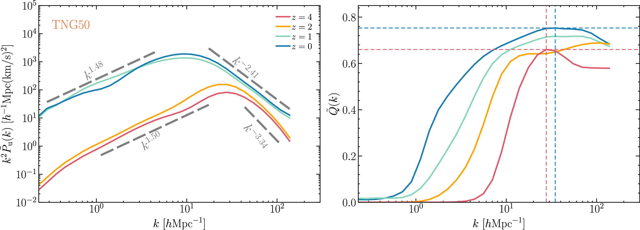
Figure 4. The z-evolution of the energy spectrum (left-hand panel) and the spectral ratio (right-hand panel) for the TNG50 simulation. Similar to Figure 3, the relevant power laws are indicated in the figure.
Download figure:
Standard image High-resolution imageFrom z = 4 to z = 0, the peak scale of the spectrum increases from kS−peak = 27.7 h Mpc−1 to kS−peak = 8.8 h Mpc−1, and the transition scale from the compressive mode to the solenoidal mode also increases from ktrans = 14.2 h Mpc−1 to ktrans = 2.7 h Mpc−1, while the peak scale of  decreases from kQ−peak = 27.7 h Mpc−1 to kQ−peak = 34.9 h Mpc−1. Additionally, it can be seen that the exponent of the spectra at small scales becomes less steep as the redshift decreases.
In Figure 5, we show the global kurtosis as a function of k for the z = 0 TNG50 data. We can see that the three directions give almost the same results, so we will only use the z-direction data in the following calculation. For the u field, it can be seen that the kurtosis = 3 at about k = 0.2 h Mpc−1, then grows rapidly with k to about ktrans = 2.7 h Mpc−1, and then grows slowly to the large-k end, indicating that the cosmic fluid becomes increasingly intermittent as k increases. As can be seen from the results for u ⊥ and u ∥, the kurtosis for u ⊥ is generally greater than that for u ∥. From the energy spectra of u ⊥ and u ∥ in Figure 3, we know that u ∥ predominates in the spectra when k < ktrans, but the kurtosis of u ⊥ is relatively significant. Consequently, the overall kurtosis can be considered a compromise between the contributions from u ⊥ and u ∥. This compromises accounts for the rapid increase in the global kurtosis observed in k < ktrans. In the range k > ktrans, u ⊥ predominates in the spectra, and hence the global kurtosis follows that of u ⊥, explaining the slow growth of the global kurtosis in this scale range.
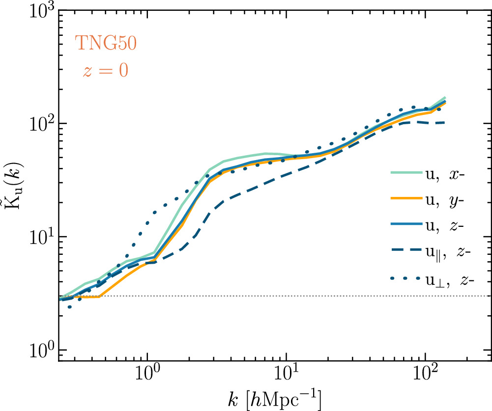
Figure 5. The global kurtosis of the velocity field u , u ∥, and u ⊥ of the TNG50 data at z = 0, respectively. The curves show the x-, y-, z-direction of u and the z-direction of u ∥ and u ⊥, respectively. The horizontal dotted line shows the kurtosis = 3.
Download figure:
Standard image High-resolution imageIn Figure 6, we show the z-evolution of the global kurtosis as a function of k for the TNG50 data. One can see that for all four redshifts the kurtosis increases with k, just as for z = 0, first in a fast mode, then in a slow growth mode. As previously analyzed, the transition scales ktrans = 14.2, 7.9, 5.0, and 2.7 h Mpc−1 for z = 4, 2, 1, and 0, respectively, roughly corresponding to scales where the fast growing mode switches to the slow mode.
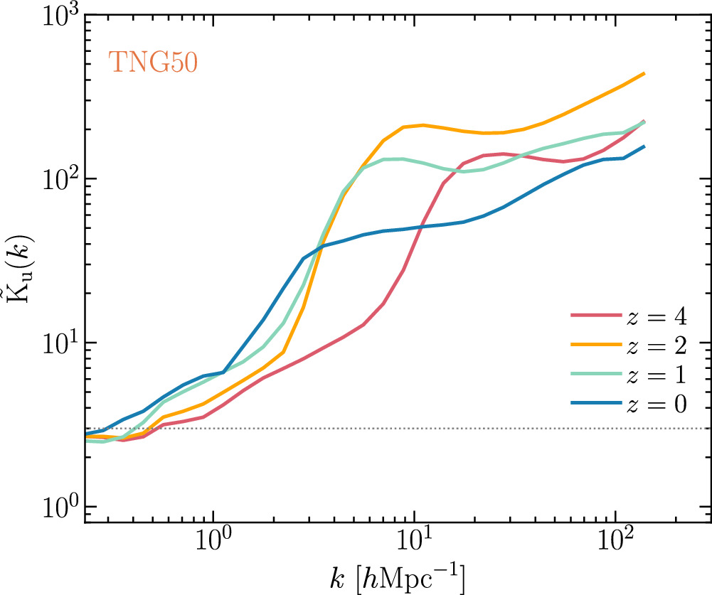
Figure 6. z-evolution of the global kurtosis for the TNG50 data. The horizontal dotted line shows the kurtosis = 3.
Download figure:
Standard image High-resolution imageAt large scales of k < 3 h Mpc−1 the kurtosis increases monotonically with decreasing z, whereas at small scales of k > 3 h Mpc−1 the kurtosis does not change monotonically with decreasing redshift—from z = 4 to 2 the global kurtosis first increases and then decreases at z < 2. These results show how the intermittency of turbulence for cosmic fluid evolves with redshift.
3.2. The Environment-dependent Results
We divide the simulation space of TNG50 into five different environments according to the dark matter density, denoted as Δi with i = 0, 1,...,4 and listed in Table 1. Among them, Δ0 and Δ1 can be regarded as voids or low-density regions, and Δ4 as various high-density structures, such as clusters, filaments, sheets, and their outskirts (see the bottom right-hand panel of Figure 1).
Table 1. The Local Density Environments, Specified With  of Dark Matter
| Δ0 | Δ1 | Δ2 | Δ3 | Δ4 | |
|---|---|---|---|---|---|
| Δdm ∈ | [0, 1/8) | [1/8, 1/2) | [1/2, 2) | [2, 8) | [8, +∞) |
Download table as: ASCIITypeset image
In Figure 7, we show the z = 0 energy spectra of the velocity field u for the five environments of TNG50. We observe that, similar to the global energy spectra in Figure 3, the env-dependent spectra also exhibit peaks. The positions of these peaks are kS−peak = 8.5, 9.5, 10.4, 11.1, and 11.8 h Mpc−1 with increasing environmental density, respectively, indicating a trend for kS−peak to shift toward larger values of k. These five env-dependent energy spectra, starting from the same k, increase with the increasing k, reach their peaks, and then decrease rapidly. These spectra are regularly distributed—the spectrum with the lowest density at the bottom and the spectrum with the highest density at the top. These results suggest that the cosmic fluid is more turbulent in a high-density environment than in a low-density environment. We also observe that the exponents of all the spectra are steeper than the Burgers exponent. Notably, the exponent in the low-density environment is even steeper than in the high-density environment, suggesting a more efficient energy transfer in a low-density environment.
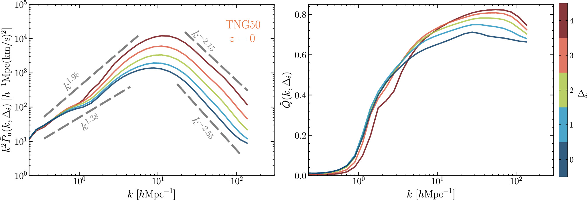
Figure 7. The environment-dependent wavelet energy spectra of the TNG50 simulation at z = 0 for the velocity field u of the cosmic fluid (left column), with the corresponding spectral ratios (right-hand column). The five environments are indicated on the color scale on the right side.
Download figure:
Standard image High-resolution imageFrom the env-dependent  , we see that the transition scale ktrans ≃ 2.7 h Mpc−1 is nearly identical for the low-density environments Δ0, Δ1, Δ2, and Δ3. This suggests that
  is insensitive to the environmental density in the scale range k < 3 h Mpc−1 when Δdm < 8. However, ktrans does depend on environmental density. For instance, in the highest-density environment Δ4, ktrans = 3.4 h Mpc−1, corresponding to ∼1.8 h−1 Mpc, roughly the outer region within a galaxy cluster. When k > 20 h Mpc−1,
  becomes sensitive to environmental density, which increases from low- to high-density environments, implying that the solenoidal mode of the velocity field is more significant in high-density environments than in low-density environments. Similar to the global spectral ratio
  shown in Figure 3, the env-dependent ratios
  also exhibit peaks. The peak positions, kQ−peak = 27.7, 32.2, 42.5, 51.0, and 55.5 h Mpc−1, respectively, shifting to higher values with increasing environmental density.
We observe that the energy spectra for the five density environments are quite similar, differing only in the peak position and the amplitude of the spectra. Turbulence can emerge in a dark matter void for the following reasons. First, even in a dark matter void, there is still a large amount of baryonic matter, as can be seen from the baryon fraction verse dark matter density in Figure 7 of H.-Y. Yang et al. (2020). Second, mathematically, when Reynolds number is sufficiently large, say  , the solutions of the hydrodynamical equations will be turbulent. Since the viscosity in the cosmic baryonic fluid is very low, TNG employs the moving-mesh code AREPO to solve the cosmological, gravo-magnetohydrodynamical equations, disregarding viscosity. Hence, it is not difficult for a flow with low viscosity to develop into turbulence, even in low-density regions.
In Figure 8, we show the z-evolution of the env-dependent energy spectra and the spectral ratios  for TNG50 data from the three environments Δ0, Δ2, and Δ4, respectively. In k < kS−peak, all env-dependent spectra grow slightly from z = 4 to 2, but are significantly enhanced from z = 2 to 1, and the spectra remain almost unchanged from z = 1 to 0. In k > kS−peak, these energy spectra are also enhanced from z = 2 to 1, but the enhancement is less than for k < kS−peak. From z = 4 to z = 0, both the peak scales of the spectra and the transition scales increase, while the peak scales of
  decrease. It can be seen that, for all the environments, the transition scales increase as the redshift decreases. Also, the exponents of all the spectra at small scales become less steep with decreasing redshift. In general, the z-evolution of the env-dependent energy spectra and spectral ratios is similar to the z-evolution of the global energy spectra and spectral ratios in Figure 4.
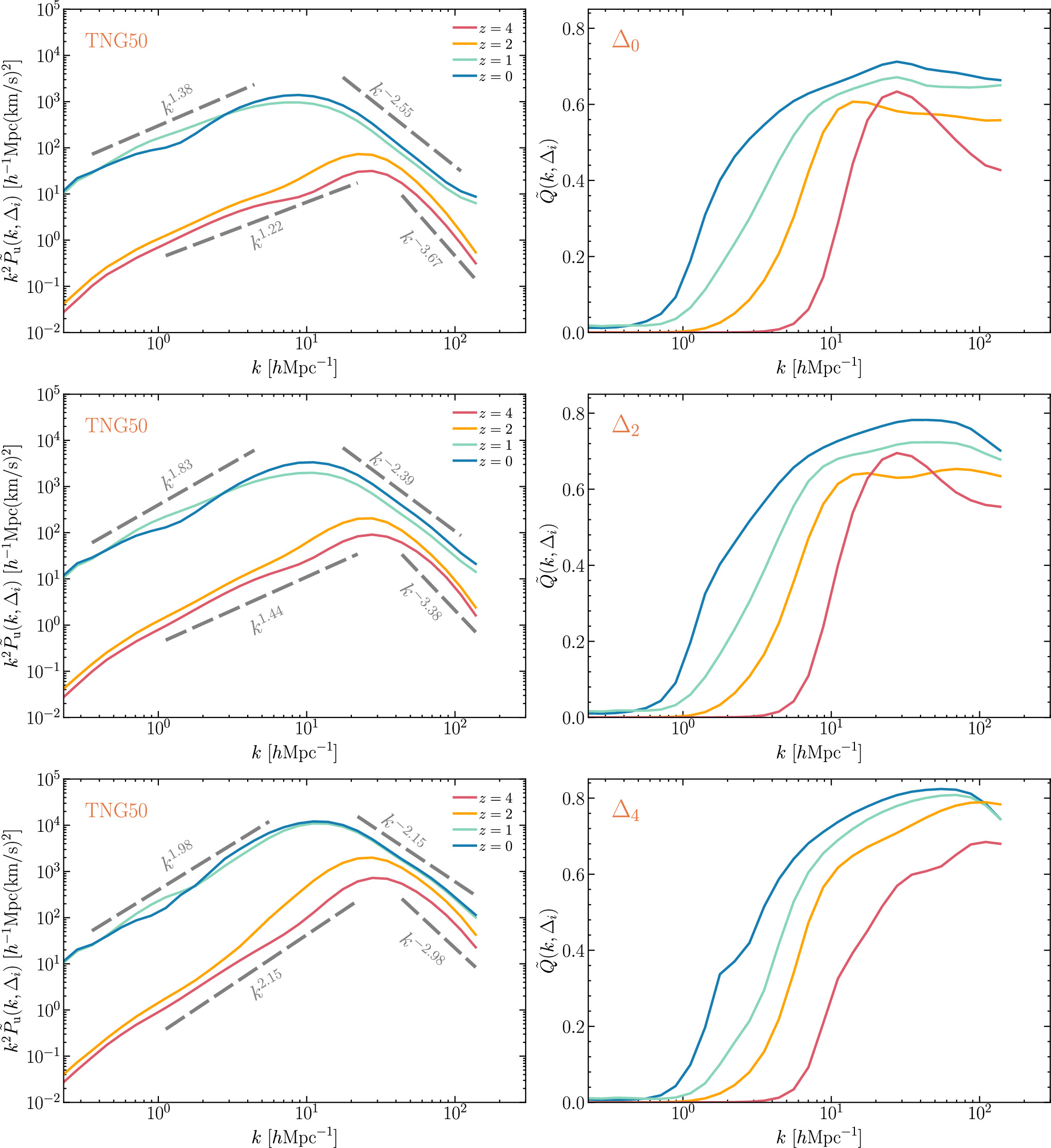
Figure 8. z-evolution of the energy spectrum (left-hand column) and the spectral ratio (right-hand column) for the TNG50 simulation of the three environments Δ0, Δ2, and Δ4, respectively. The four redshifts are shown in the figure. As in Figure 3, the relevant power laws are indicated in the figure.
Download figure:
Standard image High-resolution imageIn Figure 9, we show the env-kurtosis for z = 0 TNG50 data. It can be seen that these env-dependent results are all similar to the global kurtosis—a fast growing mode followed by a slow growing mode roughly at the transition scale ktrans as k increases. However, the kurtosis is largest for the lowest-density environment Δ0 and decreases toward the highest-density environment Δ4. The results indicate that the velocity field's intermittency in k > ktrans becomes weaker with increasing environmental density. This trend suggests an inverse relationship between the level of intermittency and the proportion of the solenoidal mode in the energy spectra, as observed by comparing the spectral ratios in Figure 7. In Figure 10, we show the z-evolution of the env-kurtosis for the three environments Δ0, Δ2, and Δ4. In general, these results are similar to the z-evolution of the global kurtosis shown in Figure 6, except for the cases of Δ0 and Δ4, where the kurtosis does not change monotonically from z = 4 to 2 at small scales of k > 20 h Mpc−1.
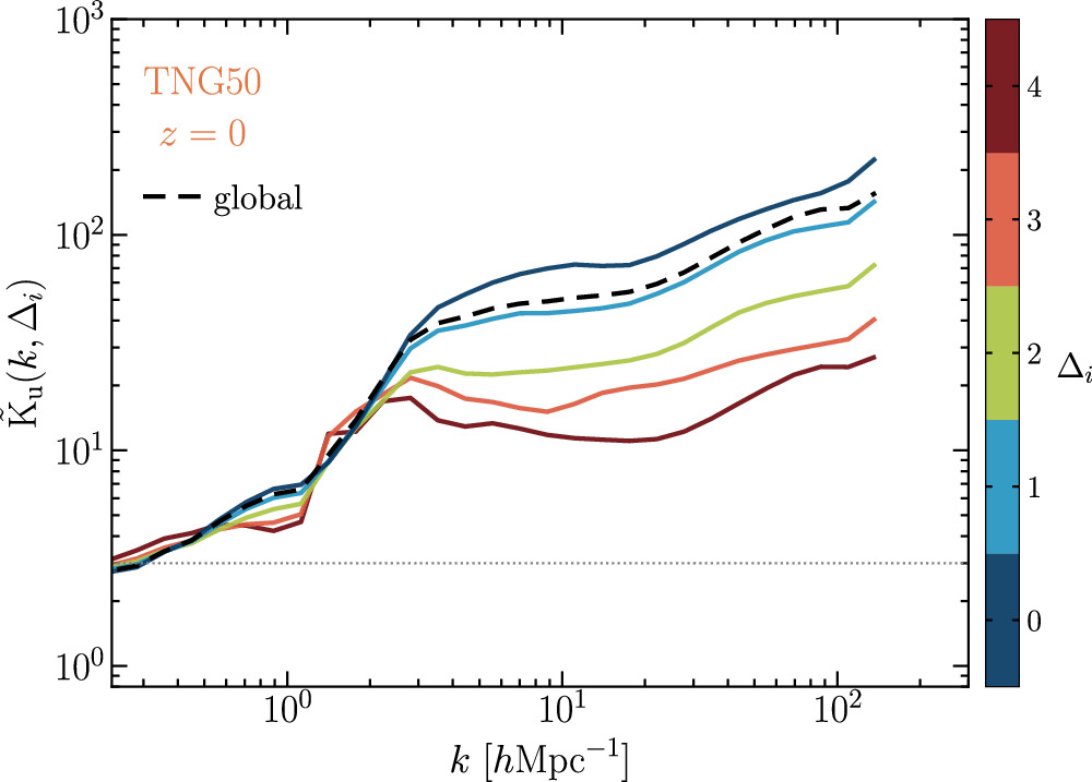
Figure 9. Environment-dependent kurtosis for the TNG50 data at z = 0. The five environments are indicated on the color scale on the right-hand side. The horizontal dotted line shows the kurtosis = 3.
Download figure:
Standard image High-resolution image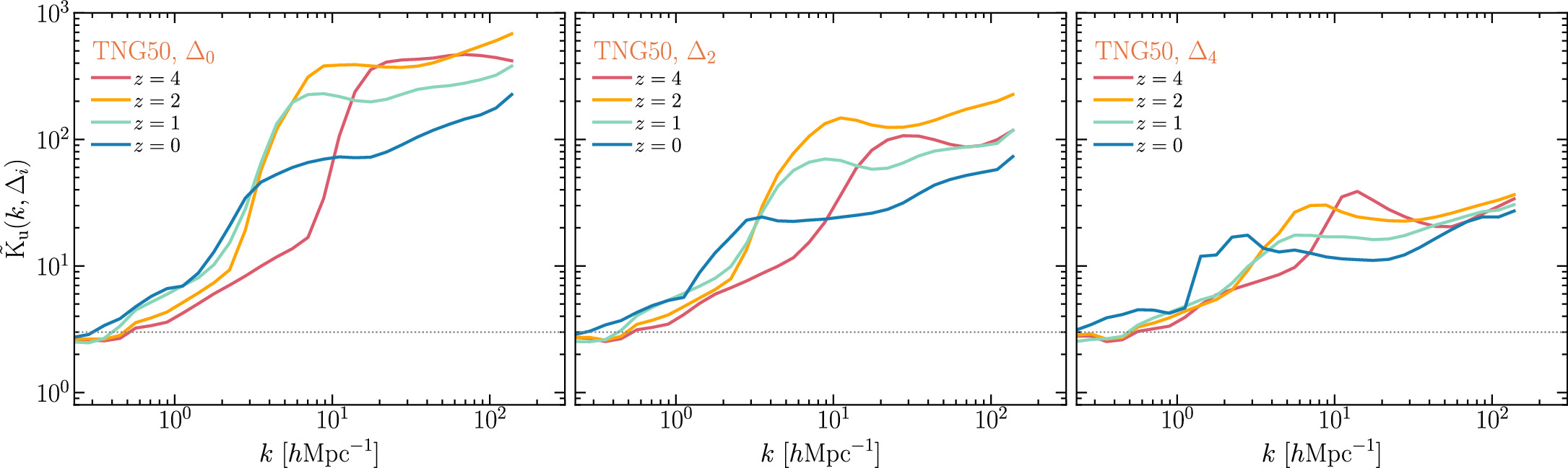
Figure 10. z-evolution of the env-kurtosis for the TNG50 simulation of the three environments Δ0, Δ2, and Δ4, respectively. The horizontal dotted line shows the kurtosis = 3.
Download figure:
Standard image High-resolution imageThese results show how the intermittency of turbulence for cosmic fluid depends on the environmental density and evolves with redshift. In general, higher kurtosis indicates a probability distribution with a sharper peak and/or heavier tails, suggesting that there are more intense events occurring within the turbulence. Intermittent events in turbulence are often associated with localized bursts of energy release, which can be identified through changes in kurtosis. Studying intermittency in cosmic fluid can have implications for cosmological models, particularly those related to the large-scale structure of the universe and the formation of cosmic structures.
4. Summary and Conclusions
The turbulent motion of the cosmic baryonic fluid, an important topic in the study of the large-scale structures of the universe, has attracted increasing attention in cosmological studies over the last few decades. In this study, we first use CWT techniques to construct the global and environment-dependent wavelet energy spectra of the cosmic baryonic fluid, which are used to characterize the intensity of the turbulence as a function of the wavenumber k. The presence of shocks leads to a strong intermittency in the baryonic fluid, so that the turbulent energy dissipation in space is also intermittent. The deviation of the tails of the PDF from Gaussian is usually considered as a manifestation of intermittency. We then define the wavelet global and environment-dependent kurtosis (or flatness) of the velocity field to characterize the intermittency of turbulence in the cosmic fluid.
We use the velocity field data from the IllustrisTNG simulation. The velocity of the baryonic fluid is decomposed into turbulent and bulk flow using the iterative multiscale filtering approach of F. Vazza et al. (2012), and the turbulent flow is further separated into compressive and solenoidal modes using the Helmholtz–Hodge decomposition.
We define five environments according to the dark matter density. We then compute both the global and environment-dependent energy spectrum and kurtosis of the turbulent velocity for z = 0 TNG data, and present the z-evolution of the turbulent energy spectrum and kurtosis. To study the contribution of the solenoidal (or compressive) mode to the total turbulence energy, we also define the spectral ratio, either the Fourier Q or the wavelet  , of the two modes of the velocity field. Our main findings and conclusions are as follows:
- 1.There are peaks in all the energy spectra at kS−peak and in the spectral ratios Q(k) and
 at kQ−peak for the velocity field of the cosmic baryonic fluid. The peak scale kS−peak can be treated as the integral scale, and the Nyquist wavenumber as the dissipation scale. Consequently, the scale range k < kS−peak, kS−peak < k <kNyquist, and k > kNyquist can be considered as the energy-containing range, the inertial range, and the dissipation range of the turbulence, respectively. In the energy-containing range, the turbulent velocity is mostly dominated by its compressive component. The gravitational collapse converts the potential energy of the structure into kinetic energy of the bulk flow, and further decays into turbulent flows, initially in the compressive mode and, as k increases, mostly in the solenoidal mode. In the inertial range, the energy passes from large-scale to small-scale eddies by the solenoidal mode or is dissipated directly into thermal energy by the compressive mode. The exponent of the energy spectrum is steeper than not only the Kolmogorov exponent but also the Burgers exponent, indicating more efficient energy transfer compared to Kolmogorov or Burgers turbulence.
 - 2.The global energy spectrum increases significantly from z = 2 to 1 in the energy-containing range, indicating that structure formation-induced turbulence is increasingly injected into the cosmic fluid with time. However, the spectrum remains almost unchanged from z = 1 to 0, indicating that the injection of turbulence by structure formation is balanced by the transfer from the larger to the smaller scales and the dissipation of turbulence into heat. In the inertial range, the energy spectrum is also enhanced from z = 2 to 1, but the magnitude of the enhancement is less than for the energy-containing range.
- 3.Similar to the global energy spectra, the environment-dependent spectra can also be classified into the energy-containing, the inertial and the dissipation range based on the two characteristic scale, kS−peak and kNyquist. The spectral magnitude is lowest in the lowest-density environment and highest in the highest-density environment, suggesting that the cosmic fluid is more turbulent in a high-density environment than in a low-density environment. In k > 20 h Mpc−1, increases from low- to high-density environments, implying that the solenoidal mode of the velocity field is more significant in high-density environments than in low-density environments. The z-evolution of the environment-dependent energy spectra and spectral ratios is generally similar to that of the global energy spectra and spectral ratios.
- 4.The kurtosis (or flatness) of the cosmic velocity field is an appropriate statistic to characterize the intermittency of turbulence in the cosmic fluid. A characteristic scale ktrans can be determined by or Q(ktrans) = 1/2. For the velocity field, the wavelet global kurtosis grows rapidly with k in the k < ktrans range, and then grows slowly in the k > ktrans range, indicating that the cosmic fluid becomes increasingly intermittent as k increases. The kurtosis for the solenoidal component is generally greater than that the compressive component. As z decreases, the kurtosis increases in the k < 3 h Mpc−1 range, whereas in k > 3 h Mpc−1 the global kurtosis first increases from z = 4 to 2 and then decreases at z < 2.
- 5.The environment-dependent kurtosis is almost completely similar to the global one—a fast growing mode followed by a slow growing mode at the transition scale ktrans as k increases. The kurtosis is lowest for the densest environment and increases toward the lowest-density environment, indicating that the intermittency of the velocity field in the k > ktrans range becomes increasingly strong as the density of the environments decreases. The z-evolution of the env-kurtosis is similar to that of the global kurtosis, except for the cases of the lowest- and highest-density environment, where the kurtosis does not change monotonically from z = 4 to 2 in the k >20 h Mpc−1 range.


Comparisons of the global WPS and the spectral ratios  with the corresponding results of the Fourier analysis show that the Fourier analysis and the global wavelet analysis give almost the same results, demonstrating that the wavelet analysis techniques are reliable and trustworthy. However, the environment-dependent wavelet analysis proves to be more powerful than the Fourier analysis in that the wavelet statistics such as the env-WPS or the env-spectral ratios
  cannot be implemented by the Fourier analysis. In this work, the environments are simply defined by the dark matter density. In fact, one can design various complex environments by specifying, for example, a particular spatial region or a specific cosmic structure.
The simple theoretical framework of turbulence is based on Kolmogorov turbulence, which is homogeneous and isotropic in space and is characterized by eddies of different scales. However, this picture is problematic for the turbulence of the cosmic baryonic fluid, which is subject to structure formation driven by gravity in the context of cosmic expansion. Structure formation leads, for example, to the density stratification of the cosmic fluid, where buoyancy forces resist radial motions, making the turbulence anisotropic (e.g., X. Shi et al. 2018; X. Shi & C. Zhang 2019; R. Mohapatra et al. 2020; M. Simonte et al. 2022; C. Wang et al. 2023). In this work, we have not yet considered the anisotropic turbulence caused by the density stratification, which will be left for future studies.
Following the general theory of Kolmogorov turbulence, we also divide the turbulent energy spectrum of the cosmic baryonic fluid into three ranges: the energy-containing range, the inertial range and the dissipation range. Note that these authors (W. Schmidt et al. 2009, 2010, 2016; X. Shi et al. 2018; X. Shi & C. Zhang 2019; X. Shi et al. 2020) also refer to these terms, but they should adopt different definitions from ours. Indeed, as X. Shi et al. (2018) points out, these concepts are not easy to identify and define. In fact, the real situation is much more complex than this general picture. Since the compressive mode exists at all scales, the kinetic energy of the turbulent flow, even of the bulk flow, can be directly dissipated into thermal energy at all scales.
In addition, in the inertial and dissipation range, both kinetic and thermal energy may also be injected by feedback from SN-driven galactic winds or AGN outflows, and these physical processes deserve to be studied in detail. Thus, the fact that the spectral exponent in the inertial range is steeper than that of Kolmogorov or Burgers turbulence indicates that the simple theory of Kolmogorov or Burgers turbulence does not hold for the cosmic baryonic fluid. One can speculate that a steeper energy spectrum may be of great significance for structure formation, which, for example, can lead to more efficient transfer of energy to smaller scales, potentially affecting the formation and evolution of galaxies.
Acknowledgments
The authors thank the anonymous referee for helpful comments and suggestions. We acknowledge the use of the data from IllustrisTNG simulation for this work. We also acknowledge the support by the National Science Foundation of China (No. 12147217, 12347163) and by the Natural Science Foundation of Jilin Province, China (No. 20180101228JC).
Software: NumPy 4 (S. van der Walt et al. 2011; C. R. Harris et al. 2020), nbodykit 5 (N. Hand et al. 2018), SciPy 6 (E. Jones et al. 2001), Matplotlib 7 (J. D. Hunter 2007), WPSmesh. 8 (Y. Wang & P. He 2024), Jupyter Notebook 9
Appendix A: The Match between FPS and Global WPS
There are a wide variety of wavelets, e.g., Poisson wavelet, Morse wavelet, Morlet wavelet, and b-spline wavelet, as well as CW-GDW we use here. The fact that they have different forms implies, on the one hand, that the same wavelet scale value may represent different physical scales for different wavelets, and, on the other hand, the WPS computed from different wavelets has different magnitudes. Therefore, we need to standardize the wavelet scale and the magnitude of WPS, which can be done by matching them to the wavenumber and FPS, respectively.
Following the scheme of S. D. Meyers et al. (1993) and C. Torrence & G. P. Compo (1998), we have demonstrated in Section 2.5 of Y. Wang et al. (2022) that the relationship w = cw
k between the wavelet scale w and wavenumber k can be obtained by solving  for w, where
  is the CWT of the 1D cosine function
  . With a closer look, we see that
  is equivalent to
  , and further to

In accordance with Equation (A1), we can get the value cw
≈ 0.3883 for the isotropic CW-GDW by solving  numerically.
Next, integrating both sides of Equation (6) with respect to w from zero to infinity, we have
Let  , then we have
which can be substituted into the Equation (A2) to get
where  is a constant depending on the wavelet. Using the w = cw
k and
is a constant depending on the wavelet. Using the w = cw
k and  , we further obtain
Considering the similar shapes of  and P
u
(k), the above equation implies that the integrand terms on both sides are approximately equal, i.e.,
and P
u
(k), the above equation implies that the integrand terms on both sides are approximately equal, i.e.,

in which the value of IΨ/(2π2 cw ) is roughly 1.0754 for the isotropic CW-GDW.
Note that the above procedure does not assume a particular form of the power spectrum. In fact, we can get a more accurate conclusion for the power-law spectra, P u (k) = Akn . Substituting it into Equation (6) gives

where  is a function of index n. For clarity, we list the values of
  for different spectral indices in Table A1. As can be seen, Equation (A3) holds exactly only for n = −1. However, most power spectra in the real world are more complicated than a simple power-law form, and it is not necessary or practicable to utilize a different factor value for each segment with a different index. Therefore, it is a fair approximation to match the FPS by multiplying the entire WPS by a factor IΨ/(2π2
cw
), at least for n > −3.
for different spectral indices in Table A1. As can be seen, Equation (A3) holds exactly only for n = −1. However, most power spectra in the real world are more complicated than a simple power-law form, and it is not necessary or practicable to utilize a different factor value for each segment with a different index. Therefore, it is a fair approximation to match the FPS by multiplying the entire WPS by a factor IΨ/(2π2
cw
), at least for n > −3.
Table A1. The Values of Scaling Factor  at Different Indices
| n | −3 | −2 | −1 | 0 | 1 | 2 | 3 |
|---|---|---|---|---|---|---|---|

| 1.4738 | 1.2211 | 1.0745 | 1 | 0.9763 | 0.9963 | 1.0587 |
Download table as: ASCIITypeset image
Appendix B: Relationship between Exponent of Energy Spectrum and Energy Transfer Rate
For homogeneous and isotropic turbulence, its energy spectrum in the inertial range can usually be expressed in the form of a power law as ∝k−n , such as n = 5/3, 2 to represent Kolmogorov and Burgers turbulence, respectively. A general conclusion is that a steeper turbulence energy spectrum, with n > 5/3, has a higher rate of energy transfer from turbulent kinetic energy to thermal energy. We will elucidate this point with Figure B1 below.
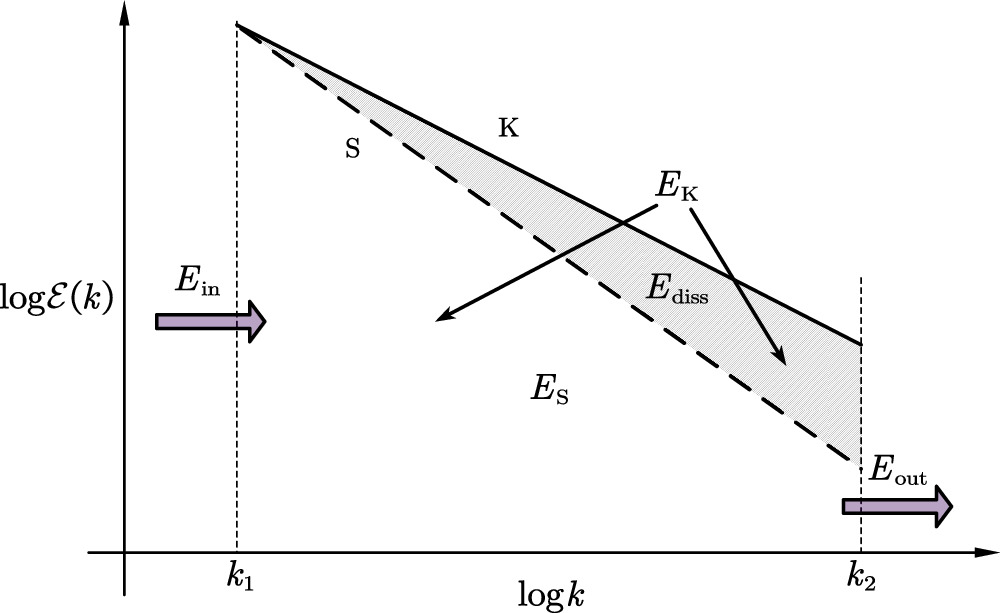
Figure B1. An illustration of the relationship between the energy spectrum’s exponent and the rate of energy transfer. “K” denotes the spectrum for Kolmogorov turbulence and “S” denotes the energy spectrum for the turbulence with a steeper exponent. k1 and k2 correspond to the integral scale lint and dissipation scale ldiss, respectively, with k1 = 2π/lint and k2 = 2π/ldiss. Ein denotes the injection energy, EK denotes the turbulent energy of Kolmogorov turbulence, ES denotes the turbulent energy of steeper-energy-spectrum turbulence, Ediss denotes the energy that is dissipated in the inertial range, and Eout denotes the energy that is dissipated at the dissipation scale k2. In the following analysis, we assume that the shapes of all energy spectra, such as the exponents and the amplitudes of the spectra, have been balanced by the continuously injected energy, thus remaining unchanged over time.
Download figure:
Standard image High-resolution imageFor a turbulent fluid system, we denote its turbulent kinetic energy as Eturb, and its energy transfer rate from turbulent kinetic energy to thermal energy at the dissipation scale k2 as ε. This energy transfer rate is a characteristic of the turbulent fluid system and should not depend on, for example, the exponent of the energy spectrum. Hence, the time it takes to transfer the turbulent kinetic energy from large-scale eddies to small-scale eddies and then dissipate it into thermal energy at the dissipation scale k2 is given by

where Eout is actually the total turbulent energy within the inertial range, i.e., Eout = Eturb. For a turbulent fluid, its turbulent energy within the inertial range is given by:

where  is the energy spectrum of the turbulence.
Since there is no energy dissipation within the inertial range for Kolmogorov turbulence, the energy transfer rate for Kolmogorov turbulence is:

where we use Equation (B1) and Ein = EK = Eout. EK is the turbulent energy of Kolmogorov turbulence, derived with Equation (B2).
Now let us turn to the case of the steeper-spectrum turbulence “S,” whose turbulent energy within the inertial range is denoted as ES, calculated with Equation (B2). From Figure B1, we know that

where Ediss is the energy that is not transferred from large-scale to small-scale eddies, but is directly dissipated into thermal energy through shock heating within the inertial range. Such processes occur within very thin fronts of shock waves and should be considered to occur instantaneously, i.e., the time taken is negligible. It should be noted that the time required to transfer energy into heat is not determined by the injection energy Ein, but by the turbulent kinetic energy Eout( = ES), as suggested by Equation (B1). Hence the energy transfer rate for the steeper-spectrum turbulence is
where we use Equations (B1), (B3), and (B4). From Equation (B5), we see that the energy transfer rate for the steeper-spectrum turbulence is larger than that for Kolmogorov turbulence.
This is precisely our conclusion that for homogeneous and isotropic turbulence, a steeper energy spectrum of turbulence indicates a more efficient energy transfer.
Footnotes
- 3
The Nyquist wavenumber, kNyquist ≡ π/Δg, is 23.5, 64.3, and 137.8 h Mpc−1 for TNG300, TNG100, and TNG50, respectively.
- 4
- 5
- 6
- 7
- 8
- 9