Abstract
The afterglow of GRB 190114C has been observed at 60–1200 s after the burst in the sub-TeV range by the MAGIC Cerenkov telescope. The simultaneous observations in the X-ray range, which is presumed to be of synchrotron origin, and in the sub-TeV range, where the emission is presumed to be inverse Compton, provide new stringent constraints on the conditions within the emitting regions and their evolution in time. While the additional data contain a lot of new information, it turns out that fitting both the X-ray and the TeV emission is much more complicated than what was originally anticipated. We find that optical flux measurements provide important complementary information that, in combination with TeV measurements, breaks degeneracy in the parameter space. We present here a numerical fit to the multiwavelength observed spectrum using a new code that calculates the single-zone synchrotron including self-Compton emission, taking into account the exact Klein–Nishina cross sections, as well as pair production via absorption of the high-energy photons inside the emitting zone and the emission from the resulting secondary pairs. We also present a revised set of single-zone parameters and a method for fitting the data to the observations. Our model for GRB 190114C that fits all the observations, from the optical data point to the sub-TeV range, suggests that it is in the fast-cooling regime. The inferred parameters for observations at two separate moments of time show significant deviations from some of the common expectations in afterglow modeling but are all consistent with the predictions of the pair-balance model.
1. Introduction
Gamma-ray bursts (GRBs), both short (that last a fraction of a second) and long (up to hundreds of seconds) ones, are followed by long-lasting multiwavelength afterglows that have been observed in X-rays, IR/optical/UV, and radio. The observations have been interpreted as synchrotron emission arising from a relativistic blast wave propagating into the interstellar medium (ISM) or stellar wind (Mészáros & Rees 1997; Sari et al. 1998). The blast wave generates magnetic fields and accelerates electrons that produce this radiation. While numerous modifications and extensions to this model have been suggested, and while some observations in various bursts do not conform to the simplest version of this model, its predictions are in rough agreement with the observations.
The basic afterglow model (Sari et al. 1998; Granot & Sari 2002) is a one-zone model where energetic electrons downstream of a relativistic shock emit synchrotron radiation in a shock-generated magnetic field. The electrons’ and magnetic energies are related to the total energy behind the shock using constant equipartition parameters. Depending on parameters, the system can be in fast or slow cooling (in the former case most of the electrons’ energy is emitted within a dynamical timescale; in the latter it is not) or in an adiabatic or radiative evolution (in the former case the blast wave energy is much larger than the radiated energy; in the latter, which can take place only in fast cooling, a significant fraction of the blast wave energy is radiated in a dynamical timescale).
The model results in closure relations between the spectral indices in different spectral ranges and the temporal behavior. While the model has been giving a good overall fit to the observations, there are well-known deviations from its basic version (plateaus, sharp decline, flares, and others). In spite of those, it has been extensively used to infer the conditions within the afterglows’ emitting regions and other global parameters, such as the total kinetic energy of the blast wave or the density distribution of the circumburst matter (see, e.g., Wijers & Galama 1999; Panaitescu & Kumar 2000, 2002; van Eerten et al. 2012; Nava et al. 2013; Beniamini et al. 2015; Ghirlanda et al. 2018; Aksulu et al. 2020, and many others).
The same electrons that produce synchrotron emission will also produce inverse Compton (IC) radiation (see, e.g., Sari et al. 1996; Panaitescu & Mészáros 1998a; Sari & Esin 2001; Pe’er & Waxman 2005; Ando et al. 2008; Fan et al. 2008; Nakar et al. 2009, and many others for discussion in the context of GRBs and their afterglow). Furthermore, Derishev et al. (2001) have shown that typical GRB synchrotron emission must be accompanied in the TeV range by an IC component, whose power is at least ∼10% of the synchrotron power. Thus, observations of the high-energy component would add significant new constraints on the emission mechanism and will enable a clearer determination of the conditions within the emitting region, such as the ratio of electrons to magnetic energy densities and the typical Lorentz factors of the emitting electrons. However, it turns out that a determination of expected spectrum when Klein–Nishina (KN) corrections take place is rather complicated. Analytic description of how IC losses in the KN regime influence the synchrotron part of the spectral energy distribution (SED) was given by Derishev et al. (2001) and then in greater detail and in application to the afterglow evolution by Nakar et al. (2009) (see also Fan 2010; Wang et al. 2010; Daigne et al. 2011; Barniol Duran et al. 2012; Lemoine 2015; Tak et al. 2019). In fact, as we show below, the situation is even more complicated than the analytic expectation when one attempts a full numerical solution.
In order to be as model independent as possible, we developed a method to estimate the conditions within the emitting region given an observed momentary SED combined with a set of observations at low energies (X-rays) corresponding to synchrotron and at high energies (TeV) corresponding to synchrotron self-Compton (SSC). Our analysis is generic, and our only assumptions are that the emission process is SSC and that the emission can be approximated using a single zone. As we describe the SED at a single moment of time, our best-fit parameters are independent of the assumption about temporal evolution of the system and are applicable to a wide range of situations, regardless of how the system evolves in time. The conditions can be described by just five variables: Γ, the Lorentz factor of the shock front; γm
(or γb
, which we define later); p, the characteristic Lorentz factor of the emitting electrons and the slope of the high-energy tail of the injection function; B, the magnetic field in the emitting region; and e
/
B
, the ratio of the electrons’ to magnetic field energy density.
The method is based on a new single-zone code from E. Derishev (2021, in preparation) that includes for a given injection spectrum all relevant radiation processes—synchrotron and SSC within the KN regime, pair creation by high-energy photons (as a result of their absorption inside the emitting zone), and the radiation from secondary pairs produced. We apply this method to the observed data of GRB 190114C (MAGIC Collaboration et al. 2019a) and compare our results to other modeling of this event (Wang et al. 2019; MAGIC Collaboration et al. 2019b; Asano et al. 2020).
GRB 190114C was observed by MAGIC in the sub-TeV range ≈60–1200 s after the trigger. We find that while details of our fit are somewhat different from our earlier results (Derishev & Piran 2019), which were analytic estimations based only on the preliminary GCN data, the basic features of fast cooling and a rather large value for the magnetic equipartition parameter (B
) hold.
Our results agree with the basic predictions of the pair-balance model (Derishev & Piran 2016). Note that, as stated earlier, the fitting procedure was generic and it did not assume this particular model. This model makes specific predictions about the average Lorentz factor of injected electrons and the ratio of synchrotron and IC powers. Its framework includes an “accelerator,” which supplies energy to radiating particles, and an “emitter,” which transfers energy from the particles to synchrotron and IC radiation. The interaction between the two is in the form of two-photon pair production due to internal absorption of high-energy IC photons by low-energy target photons (of synchrotron origin). A key feature of the pair-balance model is a strong shock modification, which smears out the discontinuity. The latter completely disappears if the power of high-energy (IC) radiation absorbed inside the shock is ∼15% of the shock kinetic power, switching off runaway acceleration of secondary pairs (Derishev & Piran 2016). The need to balance the accelerator’s power by pair loading results in the requirement that the emitting zone is not entirely transparent to its own IC radiation. It also drives the Lorentz factor of radiating electrons to a value that corresponds to the border between Thomson and KN Comptonization regimes for their own synchrotron radiation.
The paper is organized as follows. In Section 2 we describe the model that we use in our analysis. The method we use to fit the data to the model is described in Section 3. We discuss the SED fitting to the observations of GRB 190114C in Section 4. In Section 5 we compare our findings for GRB 190114C with some previous works. We then compare our findings with the predictions of the pair-balance model in Section 6. We summarize implications of our results in Section 7 and our conclusions in Section 8.
2. The Model
2.1. One-zone SSC Kinetic Equations
The one-zone model is the common simplest description of the emitting region. It assumes that the region is uniform and isotropic. Thus, the distribution functions for all particle species depend only on their energy and, in nonstationary cases, on time. The radiating particles are injected into the zone and escape from it after producing photons on their way. Introduction of particle escape terms of the form  approximates this situation. Note that the effective escape times for radiating particles and photons are, generally speaking, different, and this is accounted for by a geometrical factor Λ introduced below. If the emitting region is expanding, then radiating particles undergo adiabatic cooling in addition to radiative losses. This situation is approximated by adding expansion terms of the form
  (where
  and V is the comoving volume) in combination with an adiabatic cooling term for evolution of the radiating particle’s momentum,
  .
.
We include the following physical processes:
- (i)Radiative synchrotron losses, which are treated as continuous emission and enter equations as the source term for photons and cooling term for electrons.
- (ii)Comptonization, which can proceed in the KN regime. Therefore, we avoid continuous-loss approximation and use instead a collision integral for two-body collisions of electrons/positrons with photons with exact QED cross section. Compton scattering is taken into account by two corresponding collision terms in equations for the photon and radiating particle distributions.
- (iii)Two-photon pair production, which is important when Comptonization proceeds in the KN regime and cooling due to IC losses is fast compared to the effective photon escape time. Two-photon pair production is taken into account by two corresponding integral terms—the drain term in the equation for the photon distribution and a source term (which sums up with injection) in the equation for the distribution of radiating particles. Because of pair creation, we have both electrons and positrons, and we group them together as “radiating particles” or simply electrons. Radiation from secondary pairs is included in our model, and, as we show later, it plays an important role in fitting the spectrum of GRB 190114C.
We neglect pair annihilation, which is unimportant for GRB afterglows. We also neglect synchrotron self-absorption and induced scattering, and therefore our calculations are not valid below the self-absorption frequency, which is not relevant for the analysis carried out here. Finally, we neglect collective plasma effects.
The electrons’ distribution function,  , where γ is the electron Lorentz factor, satisfies, within this formulation,

where teff is the effective electrons’ lifetime,  , Qinj is the electrons’ injection rate,
  is the pair production rate, and Se
describes Comptonization losses that are treated via an electron–photon collision integral with exact QED cross section.
is the pair production rate, and Se
describes Comptonization losses that are treated via an electron–photon collision integral with exact QED cross section.  is the time derivative of γ due to synchrotron losses and adiabatic cooling (note that IC cooling is treated separately in Se
):
is the time derivative of γ due to synchrotron losses and adiabatic cooling (note that IC cooling is treated separately in Se
):

For the photon distribution function,  , where
 = E/(me
c2) is the dimensionless photon energy, we have

where Qsy and Sph are the synchrotron and IC photon sources. The geometric factor Λ reflects the difference in effective lifetimes for photons and electrons. It arises mainly as a result of the inevitable anisotropy in the photon distribution within the source. In application to GRB afterglows (i.e., relativistic expanding blast wave), the geometric factor is Λ ≈ 1 in the slow-cooling regime, and it increases logarithmically to ∼several in the fast-cooling regime (Derishev & Piran 2016, 2019).
2.2. Hydrodynamics and Model Coefficients
The kinetic description is supplemented by a description of the hydrodynamic evolution of the relativistic blast wave. The coupling between the hydrodynamics and the radiation is described by several dimensionless coefficients that are included implicitly in the formulation of the problem (Sari et al. 1998). The one-zone nature of the model implies using average (along equal arrival time surface, as well as due to finite width of the emitting region) values for the shock’s radius, kinetic energy of the shocked material, the lifetime of emitting electrons, the Doppler factor of the emitted photons, and source-frame luminosity integrated over an expanding spherical shock.
In general, these quantities can be expressed in terms of the shock front Lorentz factor Γ and observer’s time tobs. Sari et al. (1998) express everything in terms of the Lorentz factor of the shocked material, denoted  in that paper (following Blandford & McKee 1976). However, some authors use the Sari et al. (1998) formulae but with Γ instead of γ, and this is a source of confusion.
We define the factors Ci as





where M is the swept-up mass and hνobs the energy of observed photons, Lorentz boosted from hν in the emitting zone comoving frame, and
r
is the fraction of energy dissipated to radiation. The coefficients depend on the hydrodynamics (e.g., Blandford & McKee 1976), which depends in turn on the density distribution of the circumburst matter and on the radiative efficiency of the blast wave. But they also depend on different assumptions concerning averaging within the emitting zone. The dimensionless factors Ci
may incorporate the averaging along equal arrival time surfaces. More specifically, in this paper we use CR
that takes into account averaging over the arrival time, CΓ for averaging over the blueshift of νobs, and CL
for averaging over the Lorentz boost of observed flux.
At times one needs to know the effective Lorentz factor of emitting matter, Γem, i.e., the Lorentz factor that fluid immediately behind the shock front had at the moment when the shock’s radius was equal to the effective emission radius (Equation (4a)), whereas the shock itself had already expanded to radius Rsh = 2(m + 1)Γ2 ctobs/(1 + z), defined by the self-similar Blandford & McKee (1976) solution, Γ2 ∝ r−m , where m = 1 and m = 3 for an adiabatic blast wave propagating into wind-like and ISM density profiles. With the effective coefficients that we use in this paper, the Lorentz factor of the emitting matter and the shock front Lorentz factor are related as

Numerous authors considered different values for CR . Specifically, for the ISM case, Waxman (1997) gives CR = 1, while Sari (1997) gives CR = 8. In the wind case, Dai & Lu (1998) give CR = 4. Panaitescu & Mészáros (1998b) calculated luminosity-averaged factors CR for both ISM and wind cases. Other factors are usually hidden and not discussed. Sari et al. (1998) give, either explicitly or implicitly, the full set of coefficients Ci for the ISM case. Finally, E. Derishev (2021, in preparation) calculated effective values for all the coefficients for both ISM and wind cases. We use this last set of values (effective coefficients; see Table 1) in our best fits. It is important to state, however, that the specific values of these coefficients change the inferred values of the physical parameters, but they do not change the quality of the fit and the qualitative characteristics of the solution.
Table 1. Coefficients Used in Different One-zone Afterglow Models
| Density Profile | ||
|---|---|---|
| Reference | Wind | ISM |
| Sari et al. (1998), “SPN98 coefficients” hereafter |
CR
= 2,  , ,  , CL
= 17/12
a , CL
= 17/12
a
| |
| Panaitescu & Mészáros (1998b) | CR ≈ 3.1 | CR ≈ 6.5 |
| Nava et al. (2013) | CR = 4/5 | CR = 8/9 |
| Dai & Lu (1998) |
CR
= 4, 
|
CR
= 8, 
|
| Derishev & Piran (2019) |
CR
= 4,  , Ct
= 4, CΓ = 1 , Ct
= 4, CΓ = 1 |
CR
= 8,  , Ct
= 8, CΓ = 1 , Ct
= 8, CΓ = 1 |
| Current work (from E. Derishev 2021, in preparation), | CR ≈ 2.45, CE = 2/9, Ct ≈ 1.16, |
 , CE
= 6/17, Ct
≈ 0.96, , CE
= 6/17, Ct
≈ 0.96, |
| “effective coefficients” hereafter | CΓ ≈ 0.64, CL = 9/8 | CΓ ≈ 0.87, CL = 17/16 |
Notes. Note that in most cases these coefficients are introduced implicitly rather than explicitly in the corresponding papers. If a particular coefficient does not appear in a paper, neither explicitly nor implicitly, then it is not listed in the table.
a This coefficient does not appear in the paper, but rather is calculated using the same approach that was used to normalize the distribution of emitting electrons.Download table as: ASCIITypeset image
Some choices of coefficients (4) are summarized in Table 1. When attempting to reproduce fits obtained for GRB 190114C by other authors, we use the values given by Sari et al. (1998) (SPN98 coefficients; see Table 1). In the latter paper, as well as in many others, the authors consider Equation (4a) as an expression for both the effective emission radius and the shock’s radius at the moment of observation. This implies a relation between the shock’s radius, its Lorentz factor, and the upstream density that does not comply with the hydrodynamic solution of Blandford & McKee (1976) unless CR = 8 (ISM case) or CR = 4 (wind case). We follow this practice when trying to reproduce results of other authors, but our own best-fit solutions are obtained taking into account the difference between the effective emission radius and the shock’s radius.
Various authors, following Granot & Sari (2002), carried out “beyond one-zone” calculations in attempts to estimate the effects of a more realistic geometry on the resulting spectrum. However, as far as we know, there was no systematic attempt to quantify these effects in terms of the above set of coefficients and explore their effect on the resulting spectrum.
2.3. The Injection Function
Following Sari et al. (1998), the common choice for the injection function has been a power law with a lower cutoff:

where 〈γ〉 is the average Lorentz factor of the injected electrons. Here and below, in Equation (7), the injection function is normalized by integrating it over γ so that the product of this integral times the electron’s effective lifetime, teff, equals the number density of emitting electrons in the system ξe ne , where ne is the number density of all electrons that come from the upstream to the downstream.
This truncated-injection function was introduced in the context of analytic approximations, and it allows us to reduce the calculations to finding simple asymptotic forms while keeping all the essential physics. Numerical simulations allow more complicated expressions, and it makes sense to use a smooth form of the injection function. Therefore, in this paper we use the form introduced in Derishev & Piran (2016),
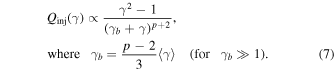
This function is differentiable in momentum space for all γ and converges to expression (6) in the limit γ ≫ γb . Being smooth, it allows one to avoid numerical artifacts that originate from the step discontinuity in the truncated-injection function.
Usually the average Lorentz factor of the injected electrons is expressed in terms of the energy fraction in accelerated electrons,

where μ is the mass per one upstream electron (μ = mp for purely hydrogen composition). The fraction of upstream electrons that are being injected, ξe , is commonly assumed to be unity. However, in the pair-balance model the injected particles originate from secondary electron–positron pairs created in the upstream, so one generally expects ξe ≠ 1 (even ξe > 1 is possible).
Whatever is the injection function, we supplement it by an exponential cutoff at the Lorentz factor

such that the synchrotron cooling rate equals the maximum acceleration rate qe
Bc and further acceleration is problematic. Here qe
is the electron’s charge, σT
is the Thomson cross section, and B is the downstream magnetic field. IC losses may decrease  . However, it happens only if IC losses are dominant even for highest-energy electrons in spite of possibly large KN corrections. This is not the case for GRB afterglows.
3. SED Fitting
We explore a stationary one-zone SSC model with effective (i.e., average) parameters to approximate the observed spectrum of a decelerating blast wave. To run ahead of ourselves a bit, this leads, for GRB 190114C, to a surprisingly good SED fit from the visible band to TeV. We estimate the goodness of SED fit in the standard way, by calculating χ2 with the set of XRT, BAT, LAT, and MAGIC observational data points; all of them are taken from MAGIC Collaboration et al. (2019b).
MAGIC Collaboration et al. (2019b) provide a table of Swift-UVOT measurements taken with a white filter and an estimate for the host galaxy extinction ( ). With these measurements we calculated the average magnitudes in two time intervals, 68−110 s and 110−180 s, which are 14.00 ± 0.03 and 14.91 ± 0.03, respectively. We converted these magnitudes into ν
Fν
values at 2 eV using UVOT white filter response,
3
correcting for extinction in our Galaxy (Schlafly & Finkbeiner 2011, about applying the Fitzpatrick 1999 model for host galaxy extinction and assuming
4
spectral index β = −0.2 (Fν
∝ νβ
)). This procedure resulted in an average ν
Fν
(2 eV) ≃ 1.14 × 10⁻⁹ erg s−1 cm−2 for the 68−110 s time interval and ν
Fν
(2 eV) ≃ 4.9 × 10⁻⁹ erg s−1 cm−2 for the 110−180 s time interval. Systematic errors due to uncertainty in the host galaxy extinction are −25% to +30%.
). With these measurements we calculated the average magnitudes in two time intervals, 68−110 s and 110−180 s, which are 14.00 ± 0.03 and 14.91 ± 0.03, respectively. We converted these magnitudes into ν
Fν
values at 2 eV using UVOT white filter response,
3
correcting for extinction in our Galaxy (Schlafly & Finkbeiner 2011, about applying the Fitzpatrick 1999 model for host galaxy extinction and assuming
4
spectral index β = −0.2 (Fν
∝ νβ
)). This procedure resulted in an average ν
Fν
(2 eV) ≃ 1.14 × 10⁻⁹ erg s−1 cm−2 for the 68−110 s time interval and ν
Fν
(2 eV) ≃ 4.9 × 10⁻⁹ erg s−1 cm−2 for the 110−180 s time interval. Systematic errors due to uncertainty in the host galaxy extinction are −25% to +30%.
The one-zone SSC model is described by four macroscopic and two microscopic parameters. The macroscopic parameters are the shock’s Lorentz factor Γ and the observation time tobs, which in turn, together with Γ, determines the lifetime of particles in the emitting zone (see Section 2.2), the magnetic field strength, and the energy density of the accelerated (injected) electrons/positrons. The last two quantities are typically expressed in terms of the equipartition parameters B
and
e
in combination with the energy density of the shocked material, which in turn is proportional to the isotropic equivalent kinetic energy of the shock, Ekin. The shock’s kinetic energy merely sets the typical GRB energy scale and has no impact on the calculated SEDs. Its value is arbitrary to a certain extent, although there are lower and upper limits based on the total observed flux and the physical model of the radiating relativistic shock. The two microscopic parameters determine the energy distribution of the leptons, which we characterize by a lower-energy cutoff at γb
(or γm
) and a high-energy spectral index of the distribution, p.
This characterization of the problem depends on the blast wave only in two ways. First, as mentioned earlier, tobs and Γ determine the leptons’ cooling time. Second, we take into account averaging over the emitting region that is reflected in the coefficients discussed in Section 2.2. We use the set of effective coefficients. In Section 4.2 we compare to the results obtained with the more familiar SPN98 coefficients. Using different coefficients leads to virtually the same SED fit, but of course the implied parameters will be somewhat different.
Our approach is to perform a systematic scan over the four-dimensional parameter space (the free parameters are Γ, B, γb
(or γm
), and the ratio of leptonic to magnetic energy e
/
B
), looking for all regions where the calculated SEDs fit the observations. We do not consider the power-law index of the injection function as a free parameter and expect that its value is universal and is dictated by the particle acceleration process, and we use p = 2.5. However, in Section (4.3) we discuss the sensitivity of our conclusions to the particular choice of p. At the same time we differ from the traditional approach by treating γb
as an independent free parameter instead of choosing the value proportional to Γ (Sari et al. 1998). As our goal is model-independent analysis, we relax the model-dependent assumption γb
∝ Γ. Similarly, when considering early and late SED fits, we do not assume a priori that the equipartition parameters remain the same. We use smooth injection (Equation (7)), but in Section 4.2.2 we compare to the results obtained with truncated injection (Equation (6)).
We calculate the SSC spectra numerically, using a newly developed single-zone code (E. Derishev 2021, in perparation), which evaluates both the underlying electron/positron distribution and the resulting photon distribution. The code takes into account synchrotron emission considering inhomogeneity of the magnetic field (assuming Gaussian distribution for its local strength, namely, 〈Bi 〉 = 0 for each component, and the rms value of the magnetic field equals B), IC scattering with recoil using the exact QED cross section, and two-photon production of electron–positron pairs (reinjected into the emitting zone), also with the exact cross section. For a given stationary injection the code finds the instantaneous SED.
We explore the full four-dimensional parameter space. This is done in two steps: first we look for a minimum χ2 in two dimensions, e
/
B
and γb
(we find that there is only one relevant minimum), and then we scan on a linear scale for Γ (the grid spacing is 5) and logarithmic for B (the spacing is 1/50 of a decade). The middle and bottom panels in Figure 1 are produced in a similar way, exchanging B with γb
or with
e
/
B
.
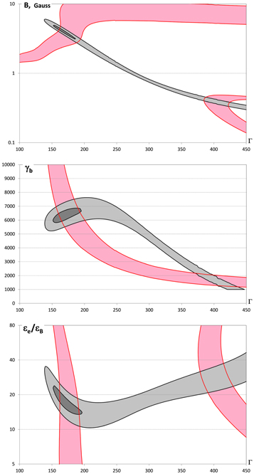
Figure 1. Regions of good fits projected onto 2D sections of the parameter space. For each pair of parameters (e.g., Γ–B in the top panel) we show a projection of the surface that passes through the best-fit values for the two other parameters (i.e., γb
and e
/
B
in the top panel). Shown are the regions of good (χ2 < 12; dark gray) and acceptable (χ2 < 16; light gray) fits to the TeV, GeV, and X-ray observations (19 data points). The region where the calculated optical flux is 0.7–1.35 of the observed value (covering both systematic and statistical uncertainties) is colored light red. Top: B–Γ parameter plane. Middle: γb
–Γ parameter plane. Bottom:
e
/
B
–Γ parameter plane.
Download figure:
Standard image High-resolution image4. Modeling GRB 190114C
We turn now to applying our method to fit the observed spectrum of GRB 190114C. The results of parameter space scans are presented in the following subsections. The case of the early-time (68–110 s after the trigger) SED fit is described in greater detail. It serves both as a practical example of our approach and as the reference for further analysis. We find the best-fit parameters for the early time and the best-fit parameters for the late time (110–180 s), as well as joint fit parameters corresponding to an adiabatic evolution between the early and late times. While the parameter groups are not that different from each other, we use the latter as our “preferred set of parameters” (see Table 2).
Table 2. Summary of Afterglow Parameters Found for a Combined Best-fit Solution at Two Moments of Time Assuming Adiabatic Evolution of the Shock Wave
| Parameter | tobs = 90 s | tobs = 145 s |
|---|---|---|
| Γ |
 ( ( ) ) |
 ( ( ) ) |
| B |
 G ( G ( G) G) |
 G ( G ( G) G) |
|
|
 ( ( ) ) |
 ( ( ) ) |
| γb |
 ( ( ) ) |
 ( ( ) ) |
| p | 2.5 | 2.5 |
| Ekin | 3 × 1053 erg | 3 × 1053 erg |
|
| 0.0061 (0.0062) | 0.0027 (0.0026) |
|
| 0.12 (0.13) | 0.096 (0.107) |
 (wind) (wind) |

|

|
| n (ISM) | 2 cm−3 | 2 cm−3 |
Note. In the table, parameters obtained with a wind density profile are followed in parentheses by parameters obtained with an ISM density profile. Note that the parameters below the double line depend on the specific choice of the shock’s kinetic energy. The errors given in the table correspond to +1 increase in χ2 measure. Note, however, that they are projections of the allowed region onto corresponding axes, and this region is elongated and inclined, so that the errors are strongly correlated. For example, the quantity Γ2.3 B is limited to within ±5% at early time and to within ±10% at late time.
Download table as: ASCIITypeset image
4.1. The Best-fit SED at Early Time
We approximate the earliest available data set, 68–110 s after the trigger, with instantaneous SED calculated for tobs = 90 s. Even though we fit an instantaneous spectrum, the effective coefficients used in the fit depend on the blast wave history. This in turn depends on the circumburst density profile. The results presented in this subsection are for a blast wave propagating into a wind external density profile. The ISM case is discussed in Section 4.2. When considering instantaneous spectra, the different coefficients lead to slightly different inferred physical parameters, but the SED itself remains essentially the same.
The best (minimal) SED χ2 values achieved in our parameter space scans are shown in Figure 1. Each point in the plots represents a solution obtained for two given parameters (say, Γ and B in the top panel), where we optimize the fit over the two other variables (γb
and e
/
B
in that case). Three conclusions immediately follow from these plots.
First, the parameter space region, where we find reasonably good SED fits, is strongly elongated. It extends from Γ ≃ 140, which corresponds to the fast-cooling regime, upward. There, starting from Γ ≃ 270, the solution becomes slow cooling. Although the best fit is firmly located at Γ ≃ 165, our fits can accommodate any Γ ≳ 140 within the range that we have explored (100 ≤ Γ ≤ 450), even though we have combined X-ray, GeV, and TeV observations. On the lower Γ values side, the allowed region is limited by internal two-photon opacity. A significant pair production would result in electromagnetic cascade, which is constrained by the LAT measurements and by the curvature of the X-ray spectrum. On the high-Γ side, the limiting factor is the hardness of the TeV tail, which, however, has rather weak statistical support.
Second, the most stringent lower limit on the shock’s Lorentz factor, Γ ≳ 160, arises from the visible-band observations. These observations put an upper bound on the contribution of secondary pairs to visible light. And in turn, this limits the amount of internal two-photon absorption and secondary pair creation to a level much smaller than the one allowed by the IC peak shape. Surprisingly, the most stringent upper limit on the shock’s Lorentz factor, Γ ≲ 420, also derives from the intersection of the allowed visible band with the allowed region from X-rays and TeV (see Figure 1). The large-Γ fits are slow-cooling solutions, and the position of X-ray peak is associated with the cooling Lorentz factor γc, whereas γb has to be much smaller (as dictated by the location of IC peak). This eventually increases the power of the optical-band emission to unacceptably high levels.
Third, the parameters of the SED fit, which reproduces the observed visible light flux in addition to X-ray and TeV spectra, are close to those of the best fit based on X-ray to TeV data points alone. Thus, there exists a good SED fit that reproduces observations in a very broad range, from ∼1 to ∼ 1012 eV.
A narrow valley of good fits extends from the global χ2 minimum near the lowest allowed shock’s Lorentz factor toward the largest possible Γ. At both ends we find an SED fit that reproduces the observed visible-band luminosity in addition to fitting the X-ray, GeV, and TeV data points. The statistically significant global minimum of χ2 (with respect to the X-ray to TeV data) falls in the region with a good fit to the optical. Solutions with lower and higher Γ are ruled out by producing too much optical radiation. Any solution from the valley of good fits between the two optically consistent SEDs provides a reasonably good fit from X-rays to TeV, which is likely the reason why different attempts to fit the SED of GRB 190114C in the literature resulted in different parameters. In the middle of the valley the predicted optical-band flux is so low that one needs another independent source of visible light.
It is interesting to analyze how restrictive is the requirement to fit the X-ray data points, ignoring other information and how much observations in various spectral bands contribute to our ability to pinpoint the GRB parameters. Figure 2 demonstrates that the X-ray data are not at all restrictive—we were able to find excellent SED fits for virtually any combination of the shock’s Lorentz factor and the magnetic field strength by varying just two remaining parameters, γb
and e
/
B
. When the (single) GeV observation is added to the X-rays, it excludes some regions at outskirts, most notably at small Γ, but still a huge degeneracy remains. The optical observations provide an even stronger constraint on the lowest possible Γ and exclude extremely strong magnetic field, which results in stronger optical signals than the one observed (a similar issue arises for the prompt phase; see Beniamini & Piran 2014). Within the hatched area shown in Figure 2 there is a good fit to the X-ray, but the optical flux produced is too low. This region is still allowed, as one can consider an additional source of visible light (“thermal” electrons, reverse shock, etc.) that contributes in the optical. On the other hand, regimes in which too much optical emission is produced (outside the red arc and the hatched region) are ruled out. Eventually, the most stringent constraint comes from TeV-range data points—the only observations that directly capture the IC component in the GRB spectra. However, degeneracy with respect to choosing the shock Lorentz factor persists unless one requires that the model reproduces the observed optical flux as well. The intersection of the TeV-allowed region with the optical-band region is the critical factor that determines the parameters.
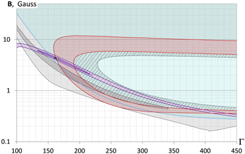
Figure 2. The parameter plane in B–Γ coordinates for tobs = 90 s, wind density profile, and smooth injection with p = 2.5. Regions where good fits to 12 X-ray data points can be obtained by varying γb
and e
/
B
are colored gray—darker shade corresponds to
 , lighter shade corresponds to
  , and the absolute minimum is
  . The blue shaded region corresponds to a good fit to the single GeV data point (
 ). Magenta shades indicate goodness of fit for six sub-TeV data points—darker shade for
  and lighter shade for
  . The light-red arc depicts the region where calculated optical flux is 0.7–1.35 of the observed value (covering both systematic and statistical uncertainties). The hatched area marks the region where there is a good fit to the X-ray data but the calculated optical flux is lower than observed. The open circle shows the location of the best fit to X-ray, GeV, and sub-TeV data points, and the nearby cross shows the solution that we choose taking into account later-time (tobs = 145 s) data points.
Download figure:
Standard image High-resolution imageThe best-fit spectrum over the whole parameter space shown in the top panel of Figure 3 corresponds to Γ = 165. However, keeping in mind the necessity of fitting the SED at a later time with the same circumburst medium parameters, we choose instead a solution corresponding to the smaller shock’s Lorentz factor, Γ = 161, and with a slightly larger value of χ2 as our reference early-time SED fit. In both these fits  , where Bcr ≈ 4.4 × 10¹³ G is the critical (Schwinger) magnetic field. This relation,
  , is a coincidence within the common model, but it is a prediction of the pair-balance model.
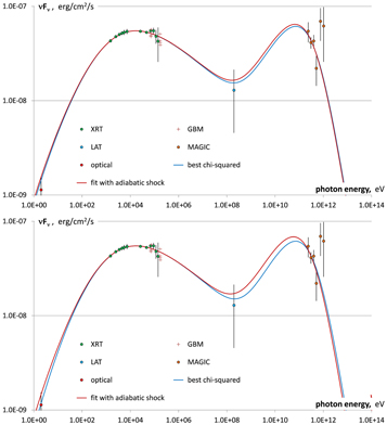
Figure 3. A comparison of the best χ2 SED fits to X-ray, GeV, and TeV data points at tobs = 90 s (blue curves) with SED fits that correspond to adiabatic blast waves with the same circumburst density parameters for both early and late observations (red curves) for the progenitor’s mass-loss rate (1.4 × 10⁻⁶
Vw,3000
E53.5
M☉
−1) or fixed ISM density (2 E53.5
mp
cm−3). Top: wind density profile. Best-fit parameters are Γ = 165, B = 4.18 G (B
≃ 6.4 × 10⁻³/E53.5),
e
/
B
≃ 18.5, γb
≃ 6620, resulting in χ2 ≃ 11.4 for 19 data points (not counting the optical point) with four parameters. The fixed progenitor’s mass-loss rate fit parameters are Γ = 161, B = 4.37 G (
B
≃ 6.1 × 10⁻³/E53.5),
e
/
B
≃ 19.6, γb
≃ 6540, resulting in χ2 ≃ 11.4 for 19 data points (not counting the optical point) with four parameters. Bottom: ISM density profile. Best-fit parameters are Γ = 115.5, B = 4.99 G (
B
≃ 6.7 × 10⁻³/E53.5),
e
/
B
≃ 19.0, γb
≃ 5570, resulting in χ2 ≃ 11.2 for 19 data points (not counting the optical point) with four parameters. Fixed ISM density fit parameters are Γ = 109, B = 5.68 G (
B
≃ 6.2 × 10⁻³/E53.5),
e
/
B
≃ 21.4, γb
≃ 5700, resulting in χ2 ≃ 11.5 for 19 data points (not counting the optical point) with four parameters.
Download figure:
Standard image High-resolution imageThe second optically consistent solution that we find at the high-Γ end of the valley of good fits corresponds to the slow-cooling regime. This solution has markedly worse goodness of fit as compared to the lower-Γ solution. It requires larger B
(and, correspondingly, larger
e
). The very large Γ in this solution implies unreasonably small circumburst density.
In Figure 4 we show the effect of internal absorption and consequent radiation from secondary pairs. In addition to flux decrease at TeV energies, the internal absorption causes an increase of flux at GeV and especially at IR–optical energies—there one sees extra radiation from secondary pairs, through IC and synchrotron emission, respectively. A small decrease at X-ray energies is because electrons cool faster in the presence of the additional radiation from the secondaries. All these effects become much more pronounced with lower values of Γ.
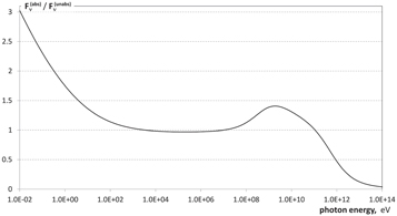
Figure 4. A comparison of fluxes produced in two simulations with identical parameters with internal two-photon absorption and with consequent radiation from secondary pairs  and without these effects
  . The parameters are from Table 2 (wind density profile, tobs = 90 s). In this particular example we use Γ = 161. The effects are more (less) pronounced with lower (higher) values of Γ.
Download figure:
Standard image High-resolution image4.2. Varying the Model Coefficients
4.2.1. ISM External Density Profile
Extending the results obtained in Section 4.1 for the wind-type external density profile to the case of constant external density (ISM case for short) requires nothing more than replacing the set of coefficients according to Table 1. Using the coefficients for the ISM case, we arrive at very similar results (see Figure 5): the allowed (good χ2 for X-ray, GeV, and TeV data points) solutions are located within a narrow band extending from the shock’s Lorentz factor Γ ≃ 95 upward, with fast-cooling (i.e., having low Γ) solutions being preferred, 5 and the best fit based on a combination of X-ray, GeV, and TeV data points (see bottom panel of Figure 3) is very close in parameter space to the solution that reproduces the observed optical flux. The physical conditions in the emitting zone are similar to those obtained in the wind case. Note that with the effective coefficients that we use, the effective emission radius is smaller than the shock’s radius, and the Lorentz factor of the emitting matter at the effective emission radius is larger than implied by the shock front Lorentz factor (due to deceleration; see Equation (5); it is Γem ≃ 149 in the wind case and Γem ≃ 141 in the ISM case).
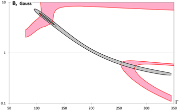
Figure 5. Regions of good fits in the B–Γ parameter plane obtained using the effective coefficients for the ISM density profile (i.e., same as the top panel of Figure 1, but for constant external density). Shown are the regions of good (χ2 < 12, dark gray) and acceptable (χ2 < 16, light gray) fits to the TeV, GeV, and X-ray observations (19 data points). The region where the calculated optical flux is 0.7–1.35 of the observed value (covering both systematic and statistical uncertainties) is colored light red.
Download figure:
Standard image High-resolution image4.2.2. Other Coefficients
We also look for a best-fit solution using the common SPN98 coefficients that correspond to the ISM case. The results, presented in Figure 6, are remarkably similar, in terms of the topology of the allowed and preferred regions in the parameter space, to the results obtained with the effective coefficients. The implied physical conditions in the emitting zone are different, but given the approximate nature of the one-zone model, we do not consider this difference as significant.
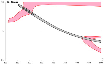
Figure 6. Regions of good fits in the B–Γ parameter plane obtained using the SPN98 coefficients for the ISM density profile (i.e., same as Figure 5, but for a different set of coefficients). Shown are the regions of good (χ2 < 12, dark gray) and acceptable (χ2 < 16, light gray) fits to the TeV, GeV, and X-ray observations (19 data points). The region where the calculated optical flux is 0.7–1.35 of the observed value (covering both systematic and statistical uncertainties) is colored light red.
Download figure:
Standard image High-resolution image4.3. Different Electrons’ Injection Function
Unlike alternative sets of the model coefficients from Table 1, choosing one or another shape of injection function causes notable changes in the topology of the allowed regions in the parameter space. Injection with p = 2.3 results in (somewhat counterintuitively) a best-fit solution with less pronounced KN corrections and a smaller rate of secondary pair production (smaller compactness). The net effect (see Figure 7) is a shift of the lower bound on the shock’s Lorentz factor to larger values Γ ≳ 180, which is again set by the observed optical flux. The best-fit region shifts to even larger Lorentz factor Γ ≃ 220 and moves away from the point that matches the optical flux, although a global fit from optical band to TeV band with reasonable goodness is still possible.
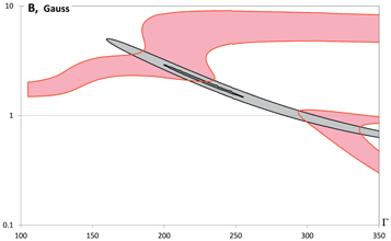
Figure 7. Regions of good fits (χ2 < 12, dark gray) and regions of acceptable fits (χ2 < 16, light gray) in the B–Γ parameter plane for hard injection with p = 2.3. The region where calculated optical flux is 0.7–1.35 of the observed value (covering both systematic and statistical uncertainties) is colored light red.
Download figure:
Standard image High-resolution imageA softer injection with p = 2.7 leads, on the contrary, to a best-fit solution with more pronounced KN corrections and a larger rate of secondary pair production. As a result, it tends to produce SEDs with too soft TeV spectra, and the region of fits with reasonable goodness shrinks to a small spot between Γ ≃ 135 and Γ ≃ 175, which again encompasses the solution that matches the observed optical flux (see Figure 8). There is also a region of lower, but still satisfactory, goodness of fit, which extends toward much larger Γ values and is a remnant of the valley-shaped region of allowed solutions found for p = 2.5 and p = 2.3. At Γ ≳ 460 there is another local minimum of χ2, which coincides with a good fit to the optical flux. However, this minimum is not as deep as the minimum at low Γ, and, in addition, it corresponds to unreasonably small external density.
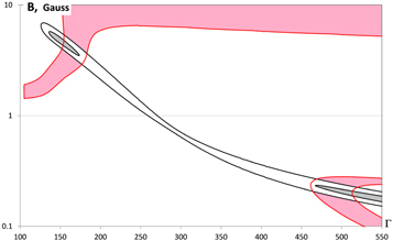
Figure 8. The regions of acceptable fits (χ2 < 16, light gray) in the B–Γ parameter plane for soft injection with p = 2.7. An additional contour line indicates a region of mediocre fits (χ2 < 25, unshaded). The region where calculated optical flux is 0.7–1.35 of the observed value (covering both systematic and statistical uncertainties) is colored light red. Note that the overall goodness of fit is lower here than in the other cases.
Download figure:
Standard image High-resolution imageFinally, we look for a truncated-injection SED fit, commonly used in most afterglow studies. Here we also find a global, from optical to TeV, fit obtained with p = 2.5. The parameters of the truncated-injection fit (see Figure 9) are not much different from those of the smooth-injection fit (note that for p = 2.5 the average Lorentz factor of injected electrons is 〈γ〉 = 3 γm and 〈γ〉 = 6 γb ). Both the smooth-injection and truncated-injection SEDs produce excellent fits to the observed optical, X-ray, GeV, and TeV fluxes and look similar in their IC part (TeV data points). The most prominent difference is the overly curved shape of the synchrotron (X-ray) peak owing its origin to the sharp cutoff in the truncated-injection function.
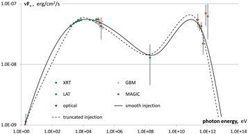
Figure 9. SED fits for smooth and truncated injection. Solid line: SED fit for smooth injection with best χ2 in X-ray, GeV, and TeV bands under the additional requirement that it exactly fits the optical-band flux (Γ = 190, B = 5.21 G (B
≃ 6.8 × 10⁻³/E53.5),
e
/
B
≃ 13.4, γb
≃ 5370). Dashed line: SED fit for truncated injection (Γ = 158, B = 6.21 G (
B
≃ 3.2 × 10⁻³/E53.5),
e
/
B
≃ 27.1, γm
≃ 21,000), which also matches the optical flux. Both fits use p = 2.5 and SPN98 coefficients that correspond to the ISM case.
Download figure:
Standard image High-resolution image4.4. Late-time SED and Evolution of the Parameters
We apply the same procedure for the later-time data set, which covers the interval from 110 to 180 s after the trigger, attempting to find the best fit with instantaneous SED calculated for tobs = 145 s. The resulting best (minimal) SED χ2 values achieved in our parameter space scans are shown in Figure 10 as a function of Γ and B. The topology of allowed regions in the parameter space is similar to those obtained with the earlier-time data set (Figures 1 and 5), and again, the best χ2 solutions based on X-ray, GeV, and TeV data points are close to the solutions that in addition reproduce the observed optical flux. The corresponding SEDs are shown in Figure 11. Thus, a later-time global SED fit from optical to TeV is possible. Like in the earlier data set, a second (slow-cooling) solution exists that provides an optically consistent fit. Again, it has worse goodness of fit, it corresponds to larger B
and
e
values, and it implies unreasonably small density of the circumburst medium.
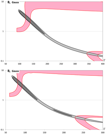
Figure 10. The SSC parameter plane at tobs = 145 s for the wind density profile (top) and ISM (constant-density) profile (bottom). The contour lines correspond to χ2 = 12 (dark gray) and χ2 = 16 (light gray) with 19 data points in X-rays, GeV, and TeV. The region where calculated optical flux is 0.7–1.35 of the observed value (covering both systematic and statistical uncertainties) is colored light red.
Download figure:
Standard image High-resolution image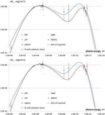
Figure 11. SED fits at tobs = 145 s. Blue lines: best χ2 SED fits to X-ray, GeV, and TeV data points. Red lines: SED fits that correspond to the same circumburst density parameters for both the early and late observations: progenitor’s mass-loss rate (1.4 × 10⁻⁶
Vw,3000
E53.5
M☉
−1) or fixed ISM density (2 E53.5
mp
cm−3). Top: wind density profile. Best-fit parameters are Γ = 115, B = 3.46 G (B
≃ 2.13 × 10⁻³/E53.5),
e
/
B
≃ 55.9, γb
≃ 15,000, resulting in χ2 ≃ 5.65 for 19 data points (not counting the optical point) with four parameters. The fixed progenitor’s mass-loss rate fit parameters are Γ = 143, B = 2.02 G (
B
≃ 2.70 × 10⁻³/E53.5),
e
/
B
≃ 35.7, γb
≃ 16700, resulting in χ2 ≃ 7.57 for 19 data points (not counting the optical point) with four parameters. Bottom: ISM density profile. Best-fit parameters are Γ = 79.1, B = 4.28 G (
B
≃ 2.14 × 10⁻³/E53.5),
e
/
B
≃ 59.0, γb
≃ 13300, resulting in χ2 ≃ 5.64 for 19 data points (not counting the optical point) with four parameters. The fixed ISM density fit parameters are Γ = 91, B=3.11 G (
B
≃ 2.62 × 10⁻³/E53.5),
e
/
B
≃ 40.9, γb
≃ 14,400, resulting in χ2 ≃ 6.74 for 19 data points (not counting the optical point) with four parameters.
Download figure:
Standard image High-resolution imageThere are several points worth mentioning when we compare earlier-time fits to later-time ones. First, the later-time fits clearly favor the smaller shock’s Lorentz factor—as expected, the shock slows down. Comparing the best χ2 solutions for early and late time, we find that they imply fast temporal evolution of Γ, faster than both wind and ISM cases for a constant-energy blast wave. This may be considered as an evidence of significant radiative energy loss, but statistical support for this conclusion is weak—it is possible to choose different pairs of solutions that obey the deceleration law of an adiabatic shock that have good χ2 values. The wind density profile solutions that we find require a reasonable mass-loss rate, and we choose them as reference solutions. Their parameters are summarized in Table 2, and the corresponding SEDs are shown in Figures 3 and 11.
We cannot choose a pair of early-time and late-time SED fits that are in good agreement with the optical observations while also obeying the adiabatic shock deceleration law, with either the wind or ISM density profile. A decrease of the shock energy with time due to radiative losses relaxes this discrepancy somewhat, so that the remaining difference in the optical-band fluxes is ∼ 20%–30%.
Based on our model SEDs we find that from tobs = 90 s to infinity ∼ 1.3 × 1053 erg was radiated, setting a lower limit for the shock energy. The best-fit parameters hint at a significant energy decrease between 90 and 145 s, so we are not far from this lower limit. Therefore, we will use Ekin = 3 × 1053 erg as a reference value, denoting it as E53.5. The best-fit solutions that are consistent with adiabatic evolution from the early to the late epoch correspond to mass-loss rate 1.4 ×10⁻⁶ Vw,3000 E53.5 M☉ yr−1 (here Vw,3000 is the wind velocity in units of 3000 km s−1) in the wind case and to density n ≃ 2 E53.5 cm−3 for the ISM. Neither wind nor the ISM is clearly preferred over the other, and we need additional arguments to tell the two cases apart.
Second, the fit parameters clearly show that the average Lorentz factor of the injected electrons increases with time, in contradiction with the usual assumption γb
∝ Γ. As the earlier- and later-time fits are consistent with  (see bottom panel of Figure 12), this implies that the fraction of accelerated electrons decreases while the shock expands. Such a strong evolution of the fraction of accelerated electrons is a natural feature of the pair-balance model (Derishev & Piran 2016). Interestingly, the fraction of self-absorbed high-energy photons is the same (≃10%) in both the late and early solutions, in line with the expectation of the pair-balance model.
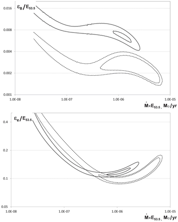
Figure 12. Regions of acceptable parameters (based on X-ray, GeV, and TeV data points) shown in B
−
 (top) and
 e
−
 (bottom) coordinates for tobs = 90 s (solid lines) and tobs = 145 s (dashed lines). The mass-loss rate is calculated assuming wind velocity Vw
= 3000 km s−1. The contour lines mark regions of good fits (χ2 < 12) and regions of acceptable fits (χ2 < 16). Note that while the allowed regions for
(bottom) coordinates for tobs = 90 s (solid lines) and tobs = 145 s (dashed lines). The mass-loss rate is calculated assuming wind velocity Vw
= 3000 km s−1. The contour lines mark regions of good fits (χ2 < 12) and regions of acceptable fits (χ2 < 16). Note that while the allowed regions for e
overlap, those for
B
do not. Radiative losses decrease the later-time shock’s energy, and hence the regions of acceptable parameters calculated for later time shift slightly upward and to the left.
Download figure:
Standard image High-resolution imageThird, the earlier- and later-time fits exclude constant B
for an adiabatic blast wave (see top panel of Figure 12). However, the condition
 holds, up to a factor of 3 for the early stage, in which
  versus γb
= 6500, and less than 2 in the late stage, in which
versus γb
= 6500, and less than 2 in the late stage, in which  versus γb
= 16,700, in agreement with the pair-balance model.
versus γb
= 16,700, in agreement with the pair-balance model.
Fourth, both early- and late-time solutions are very fast cooling (only ≃10% of the total injected power remains in the electrons). The system is relatively strongly absorbed (≃10% of the total power of injected electrons is eventually absorbed and comes out as secondary pairs at lower energies). A significant fraction of the radiation power is in the IC component (decreasing from ≃40% at early time to ≃30% at late time).
5. Comparison with Other Works
Soon after the discovery of GRB 190114C was announced, several papers analyzed the afterglow parameters, yielding significantly different results. We compare in this section some of these results with the results obtained with the code used here.
The first study of GRB 190114C afterglow parameters (Derishev & Piran 2019) was based on MAGIC detection announcement and data from the corresponding GCN messages. Since the data were preliminary and incomplete, the study did not go beyond analytic order-of-magnitude estimates, yielding, however, some nontrivial results: the shock’s Lorentz factor Γ ≃ 100 at tobs = 70 s, the effective Lorentz factor of emitting electrons γeff ≃ 104, radiation in the fast-cooling regime with Comptonization on the border of the KN regime, and unexpectedly large magnetic energy fraction B
≃ 0.1, likely reduced by a factor of several provided that the IC peak is strongly suppressed by internal two-photon absorption. Qualitatively, these results are supported by much more elaborate analysis in the present paper, although the numbers are somewhat revised—partly because the initially reported lower limit on TeV flux appeared to be more than two times smaller than the actual value and partly because of the combined action of KN corrections and internal two-photon absorption, whose influence is possible to evaluate only numerically.
We compare the SEDs calculated by MAGIC Collaboration et al. (2019b), Wang et al. (2019), and Asano et al. (2020) to SEDs calculated using our code with the same parameters. All three use ISM density profiles with the SPN98 coefficients and truncated injection. When trying to reproduce their results, we use the parameters presented in the papers and adopt the same assumptions about the density profile, the coefficients, and the shape of the injection function.
The model parameters given in Asano et al. (2020) are external density n = 0.3 cm−3, the shock’s kinetic energy Ekin = 4 × 1053 erg, observation time tobs = 80 s, e
= 0.1,
B
= 1 × 10⁻³, and truncated injection with index p = 2.3. From this set of parameters we calculated Γ = 251, B=1.2 G, and γm
= 7520. Additionally, Asano et al. (2020) assume an escape time for photons that is 6 times smaller than the lifetime of the emitting electrons. This corresponds, in our notations, to a geometrical factor Λ = 1/6 (see Equation (3)) that is hardly possible for a slab geometry.
6
The SED calculated with the above parameters (using Λ = 1/6) is in a reasonable agreement with the results of Asano et al. (2020) (see bottom panel of Figure 13). The difference between the original SED and its reproduction exceeds the anticipated precision of the code we used, and it cannot be attributed to inclusion of internal two-photon absorption in our code. However, the results can be brought to an agreement with a minor change in the parameters. Extrapolating to the usual Λ = 1 assumption, one needs about 6 times larger
B
(about 2.5 times stronger magnetic field) to obtain a similar SED. With this correction, the corresponding solution is not far from the valley of good fits that we find, although it is far from a considerably better fit found in the low-Γ end of this valley.
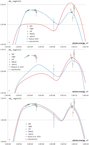
Figure 13. SEDs from MAGIC Collaboration et al. (2019b) (top panel, blue curve), Wang et al. (2019) (middle panel, blue curve), and Asano et al. (2020) (bottom panel, blue curve) and their numerical reproduction (red curves). The parameters of the emitting zone for each of the fits are given in the text.
Download figure:
Standard image High-resolution imageOne of the first attempts to explain the observations was by Wang et al. (2019), who tried to model only the TeV emission of this source. The model parameters are external density n = 0.3 cm−3, the shock’s kinetic energy Ekin = 6 × 1053 erg, observation time tobs = 90 s (in the middle of the quoted time interval 50–150 s), e
= 0.07,
B
= 4 × 10⁻⁵, and truncated injection with index p = 2.5. From this set of parameters we calculated Γ = 252, B = 0.24 G, and γm
= 7630. With the above parameters the agreement between our numerical results (see middle panel of Figure 13) and the SED presented in Wang et al. (2019) is only qualitative, with the largest deviation around the synchrotron peak. The model proposed by Wang et al. (2019) attributes the X-ray peak to a different origin. Consequently, both the original SED and—especially—its numerical reproduction fall short of the observed X-ray flux with this set of parameters.
The model parameters given in the discovery paper MAGIC Collaboration et al. (2019b) are external density n = 0.5 cm−3, the shock’s kinetic energy Ekin = 8 × 1053 erg, observation time tobs = 90 s (in the middle of the quoted time interval 68–110 s), e
= 0.07,
B
= 8 × 10⁻⁵, and truncated injection with index p = 2.6. From this set of parameters we calculated Γ = 245 (to avoid confusion, let us remind that in our notations Γ is the shock’s front Lorentz factor, which is
 times larger than the bulk material Lorentz factor immediately behind the shock), B = 0.43 G, and γm
=8350 (following Equation (8) with ξe
= 1). With the above parameters our numerical results (see top panel of Figure 13) strongly deviate from the SED presented in MAGIC Collaboration et al. (2019b), and we could not come even to a qualitative agreement by varying parameters around these values. These authors find
times larger than the bulk material Lorentz factor immediately behind the shock), B = 0.43 G, and γm
=8350 (following Equation (8) with ξe
= 1). With the above parameters our numerical results (see top panel of Figure 13) strongly deviate from the SED presented in MAGIC Collaboration et al. (2019b), and we could not come even to a qualitative agreement by varying parameters around these values. These authors find e
/
B
= 875. In the Thomson regime
 , whereas the observed value is ≈ 1. These authors suggest that KN corrections and self-absorption reduce the high-energy IC emission. However, our simulations show that the KN corrections and self-absorption are insufficient to reduce the IC flux by such a large factor. We find it to be an order of magnitude higher than the synchrotron peak flux (see red line in the top panel of Figure 13).
Figure 14 depicts a comparison of the numerical SED with SPN98 coefficients and a truncated injection with the analytic SED based on Nakar et al. (2009) using the same parameters. It is important to note here that in obtaining this SED, Yamasaki & Tiran (2021) assumed that the KN decline in the scattering cross section is abrupt and occurs at photon energy 0.2me c2 (in the electron’s frame) rather than at energy me c2 as in the original Nakar et al. (2009) formulation. This modification takes into account the fact that KN corrections begin to take place for electron energies lower than me c2. Self-absorption of high-energy photons due to pair production with low-energy photons is not taken into account in this analytic calculation. This leads to some excess of high-energy photons, as well as a lack of low-energy photons, which in the numerical calculation are produced mostly by these secondary pairs.
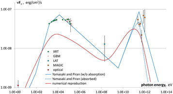
Figure 14. A comparison of the observations with numerical (red curve) and analytic (blue curve) SEDs calculated for tobs = 90 s. The analytic model Yamasaki & Tiran (2021) follows a modified Nakar et al. (2009) formulation and uses the same parameters as the numerical one. Fit parameters are the shock’s kinetic energy Ekin = 3 × 1053 erg, constant-density external medium with n = 12 cm−3, the shock’s front Lorentz factor Γ = 146, B = 4.6 G (B
= 1.1 × 10⁻³),
e
= 0.038 (
e
/
B
= 35.6), γm
= 20300, truncated injection with index p = 2.5, and SPN98 coefficients that correspond to an ISM.
Download figure:
Standard image High-resolution image6. Comparison with the Pair-balance Model
Parameters of the best-fit solution, which we find for GRB 190114C, are such that a significant fraction of radiated power is absorbed within the emitting zone by annihilation of high-energy (IC) with low-energy (synchrotron) photons producing secondary electron–positron pairs. The very same process inevitably takes place in the upstream region of the shock. A consistent description of GRB afterglows must, therefore, take this into account and suggests using the pair-balance model (Derishev & Piran 2016). In this model the pairs produced in the upstream deposit energy and momentum and modify both the hydrodynamic flow and the magnetic fields in this region (see Figure 15). Thus, the shock propagates into an already-perturbed upstream that contains a significant fraction of high-energy pairs, as well as the seed magnetic field.
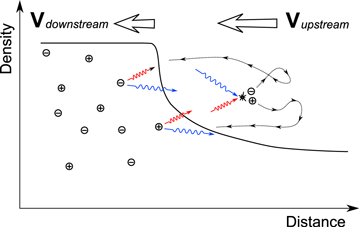
Figure 15. A sketch of the modified relativistic shock in the pair-balance model. High-energy IC photons interact with low-energy synchrotron photons ahead of the shock to produce electron–positron pairs, which are intercepted by the upstream magnetic field. The pairs transfer momentum to the upstream matter, accelerating and compressing it, so that the velocity jump at the shock front is greatly reduced. In the downstream, the pairs produce synchrotron and IC radiation. In the upstream they build up the magnetic field.
Download figure:
Standard image High-resolution imageThis leads to several important differences from the regular diffuse shock acceleration. First, the high-energy photons serve as the neutral agents that transfer energy across the shock from the downstream to the upstream region, within the converter acceleration mechanism (Derishev et al. 2003). The newly created pairs gain energy by a factor up to ∼ Γ2 once they cross the shock. In the downstream these accelerated leptons emit both low-energy (synchrotron) and high-energy (IC) photons. Some of the fresh higher-energy photons create comparable higher-energy pairs once they annihilate in the upstream. These will gain another factor up to ∼ Γ2 upon crossing the shock. In a converter acceleration the energy of the accelerated particles would diverge unless something turns down the energy transfer across the shock. Here, as the high-energy photons are produced in the downstream by IC, the process becomes inefficient once the KN regime is reached. As the low-energy photons are produced via synchrotron emission, this sets a natural limit on the typical electrons’ Lorentz factor, γb
, and the magnetic field B within the downstream region, such that  .
.
A second important and essential aspect of this model, which does not have a direct effect on the spectrum discussed here, is the decay of the magnetic field in the downstream, which takes place over a large scale. As the seeds of the magnetic field were generated in the upstream over a scale of order of the optical depth for pair creation, its decay will not be over a skin depth, but rather on a scale comparable to this macroscopic length.
Third, operation of the pair-balance model implies that a fixed and nonnegligible fraction of the high-energy (IC) photons annihilate in the upstream, producing pairs by interaction with lower-energy (synchrotron) photons. Since both the IC and the synchrotron photon field densities are similar in the upstream and downstream regions, we expect that a comparable, constant, and nonnegligible fraction of the IC photons will be self-absorbed within the downstream region as well.
Fourth, a distinct component of high-energy leptons is injected into the upstream. This breaks the one-to-one relation between the number of emitting leptons and the number of external electrons that the shock front has crossed (e.g.,  for the ISM). Put differently, this introduces ξe
≠ 1 and relaxes the common link Equation (8).
for the ISM). Put differently, this introduces ξe
≠ 1 and relaxes the common link Equation (8).
As we have seen earlier, features such as varying in time ξe
, increase of γb
while the shock decelerates, approximate equality of γb
and  , and a large (and constant) fraction of self-absorbed IC photons that emerged from the best fit to the observed data are in full agreement with predictions of the pair-balance model. On the other hand, some of these features (e.g., significant variation of ξe
and increasing γb
while Γ decreases) are incompatible with common assumptions concerning particle acceleration in shocks. Those that are compatible, like
, and a large (and constant) fraction of self-absorbed IC photons that emerged from the best fit to the observed data are in full agreement with predictions of the pair-balance model. On the other hand, some of these features (e.g., significant variation of ξe
and increasing γb
while Γ decreases) are incompatible with common assumptions concerning particle acceleration in shocks. Those that are compatible, like  , are not predicted.
7. Implications
Observation-wise, the prompt γ-rays and the low-energy afterglow of GRB 190114C are similar to those of an ordinary burst with larger-than-average luminosity. But this was a unique occasion when a GRB was detected in the sub-TeV range early in the afterglow and its simultaneous SED was measured from ∼1 eV to ∼1 TeV. We used this opportunity to analyze in unprecedented detail the best-fit SED at two moments of time. While it was generally believed that detection of both a low-energy (synchrotron) and a high-energy (IC) component would straightforwardly reveal the conditions within the emitting region, it turns out that this was not the case and this task was quite challenging.
Beyond obtaining the parameters of the emitting region in this burst, our goal was to present a new systematic method of fitting the SSC spectrum in the regime of KN correction accompanied by self-absorption of IC photons, and to compare the conditions determined for this burst with afterglow modeling. We find an excellent fit to the data all the way from optical to TeV. However, our results suggest that afterglow parameters and their evolution in time deviate from common expectations.
To make sure that we are not missing any possible solution consistent with observations, we performed a systematic scan over four-dimensional parameter space (Γ, B, e
/
B
, and γb
) that was possible thanks to the good speed of a new one-zone SSC code (E. Derishev 2021, in preparation), which we used. This scan reveals a valley of good fits—an allowed region in the parameter space, which stretches along the Γ axis, being relatively narrow in three perpendicular directions. For a fixed Γ, the valley’s extent in B,
e
/
B
, and γb
is dictated by observations of the IC (sub-TeV) component; therefore, they are crucial in determining the emitting zone’s parameters. Surprisingly, the allowed range of Γ is limited by optical observations both from above and from below. The SEDs corresponding to the low-Γ and high-Γ ends of this range match the observed optical flux in addition to fitting the X-ray, GeV, and sub-TeV data points. Therefore, the entire spectrum from 1 eV to 1 TeV is well reproduced by a single-zone model without invoking additional sources of low-energy photons.
The quality of the fit within the allowed parameter range is not uniform. The region at the low-Γ end has a significantly better goodness of fit than the one at high Γ. Moreover, the high-Γ end of the allowed parameters corresponds to unreasonably low external density. Hence, we consider the low-Γ end as the best-fit solution. Solutions at intermediate Γ are allowed by the X-ray to TeV data, but they would require an additional source of optical emission to match the observations. Solutions with higher or lower Γ values overproduce the optical signal.
With different sets of model coefficients (e.g., corresponding to either wind or ISM external density profile), the allowed region in the parameter space preserves its topology—a relatively narrow valley that stretches along the Γ axis with the best-fit solution located at the low-Γ end. Changing the injection’s power-law index away from the value p = 2.5 also preserves the topology, but the location of the best-fit solution shifts somewhat from the low-Γ end of the valley (see Figures 7 and 8), and goodness of fit is worse. Finally, we find the same topology for two moments of time that we explored—at tobs = 90 s and at tobs = 145 s.
We analyzed each of the two SEDs separately, namely, we determined the conditions at the early and late time independently of each other. It turns out that for both the early and late time the best-fit SEDs correspond to fast-cooling solutions with significant self-absorption of IC photons. Both solutions have relatively large magnetization and energy fraction in accelerated electrons (B
∼ 0.003–0.006 and
e
∼ 0.1 assuming Ekin = 3 × 1053 erg). Their ratio,
e
/
B
∼ 20–40, agrees with common expectations, but our fits suggest that it increases in time.
The early-time and late-time solutions are consistent with constant e
but, surprisingly, are not consistent with constant
B
under the assumption of adiabatic shock. The latter inconsistency suggests ≳ 20% decrease of the shock’s kinetic energy between tobs = 90 s and tobs = 145 s. These radiative losses are reasonable at such an early phase of the afterglow. Parameters of both fits approximately satisfy the relation
 . We also find that the fraction of self-absorbed photons stays approximately constant. Both features are predictions of the pair-balance model but are coincidental in others. More surprising is the fact that the fits at two moments of time also demonstrate that the average Lorentz factor of injected electrons increases in time, whereas the shock’s Lorentz factor decreases. This is counter to the common expectations but finds explanation within the pair-balance model.
The parameters of our best-fit solutions that we find under the assumption of the constant shock’s kinetic energy are summarized in Table 2. The exact values we obtain depend on the set of model coefficients that we used and on the smooth shape of the injection function that we have assumed. This treatment is meant to give us a better estimate of the conditions in the emitting region. By no means is the specific set of coefficients and specific choice of the injection function’s shape the reason for deviation from the common model—the main conclusions of incompatibility with the common assumptions are independent of these choices, and they hold, for example, for SPN98 coefficients and a truncated-injection function.
8. Summary
In this work we have used a new code (E. Derishev 2021, in preparation) to calculate the SSC spectrum and obtain a best fit to the observations of GRB 190114C. The calculations include exact KN corrections, pair production via self-absorption of the high-energy photons, and the corresponding emission of these pairs. Both the IC losses and the production of secondaries are calculated via kinetic equations with exact QED cross sections. This modified one-zone model introduces a new set of coefficients that enable us to mimic within single-zone calculations the effect of a quasi-spherical relativistic blast wave.
Our most important findings are as follows:
- 1.The best-fit solutions to the observed GRB 190114C SEDs both at tobs = 90 s and at tobs = 145 s are fast cooling (only ∼10% of the power of the injected electrons is not radiated), with KN corrections to the IC spectra and relatively strong self-absorption of IC photons (≃10% of the total emitted power, i.e., ≃25% of initially produced IC power, is absorbed in situ). They provide good fits to the observed SEDs from optical to TeV, despite that they were obtained without reference to the optical flux measurements (i.e., we find no need in an additional source of optical radiation).
- 2.We find that the afterglow blast wave of GRB 190114C had an isotropic equivalent energy of at least 1.3 × 1053 erg (and likely close to this lower limit). The afterglow blast wave was still highly relativistic Γ ≳ 160 at 90 s after the burst. A lower limit Γ > 100 was derived by Derishev & Piran (2019) ignoring optical emission from secondary pairs. The equipartition parameters are
e ≃ 0.12/E53.5,
- 3.The best-fit numerical solution that we find has characteristics similar to the analytic estimate by Derishev & Piran (2019)—it is fast cooling with significant self-absorption and Comptonization on the border between the Thomson and KN regimes.
- 4.The values for the best-fit parameters we obtain are different from those found in earlier works (Wang et al. 2019; MAGIC Collaboration et al. 2019b; Asano et al. 2020). In particular, we cannot reproduce the theoretical spectrum shown in the discovery paper (MAGIC Collaboration et al. 2019b) with their given parameters; we reproduce the TeV part shown in Wang et al. (2019), although this work does not attempt to fit both X-rays and TeV with a single source; and finally, we reproduce the spectrum presented by Asano et al. (2020) once we adopt their relation between the escape time of the electrons and the photons. However, their solution is substantially different from the best fit that we find.
- 5.The typical Lorentz factor of injected electrons, γb or γm , approximately satisfies the prediction of the pair-balance model that it should be
 , and it increases in time. Such an increase is predicted in the pair-balance model, but it contradicts the common assumption that γb
, γm
∝ Γ.
, and it increases in time. Such an increase is predicted in the pair-balance model, but it contradicts the common assumption that γb
, γm
∝ Γ. - 6.The TeV data points are the most important factor in determining the acceptable range for B,

To conclude, we note that while GRB 190114C is the first GRB detected in TeV, there is no reason to expect that it is unique. The observed deviation from common modeling assumptions may be generic, and if so, these observations suggest that we have to reconsider these assumptions. Additional detections of TeV emission from GRBs with Cerenkov telescopes and in particular the upcoming CTA may demonstrate this need in the future.
We thank Ehud Nakar, Lara Nava, Alexei Pozanenko, and Shotaro Yamasaki for helpful discussions. This research is supported by the Russian Science Foundation grant No. 21-12-00416 (E.D.) and by an advanced ERC grant: TREX (T.P.).
Footnotes
- 3
- 4
To check whether the model SED agrees with observations, we use the calculated SED slope (which is around β ≈ −0.2) to convert the actual detector response to the flux estimate. This slope agrees with the MAGIC Collaboration et al. (2019b) estimate, β = −0.10 ± 0.12, and the difference in flux estimates for β = −0.2 and β = −0.1 is ≃ 5%, which is insignificant compared to errors due to extinction uncertainty.
- 5
Like in the wind case, high-Γ solutions are in the slow-cooling regime.
- 6
Asano et al. (2020) argue that the electrons move across the emitting zone with the hydrodynamical speed c/3, while photons escape from the center of the emitting zone with the speed c along the shock’s normal, i.e., their escape time is 6 times smaller. However, first, the emitting zone’s boundary is not stationary, but it also moves away with the speed c/3. Second, photons that move at an angle to the shock’s normal escape more slowly, and in a slab geometry the effective photon lifetime averaged over different propagation angles diverges logarithmically unless one takes into account the slab’s expansion.