Abstract
Classical Ae (CAe) stars are main-sequence, A-type stars with Hα emission but no signature of dust. They are thought to be the cool extension of the classical Be stars to lower masses. Recent surveys based on Hα spectroscopy have significantly increased the number of known CAe stars, with the population extending to spectral types as cool as A4 (Teff ≈ 8500 K). We compute the temperature structure of gaseous, circumstellar disks around A-type stars, including both radiative heating from the central star and viscous shear heating from the disk’s rotation. We find that shear heating can become important for spectral types A2 and later and can act to increase the low temperatures predicted by purely radiatively heated disks. Our modeling indicates that the presence and strength of Hα emission for spectral types A2 and later significantly increases with the amount of shear heating included, and we propose that this dependence can be used to constrain the α viscosity parameter appropriate for CAe star disks.
Original content from this work may be used under the terms of the Creative Commons Attribution 4.0 licence. Any further distribution of this work must maintain attribution to the author(s) and the title of the work, journal citation and DOI.
1. Introduction
Classical Ae (CAe) stars are main-sequence, A-type stars characterized by the presence of emission lines in their spectra, most notably that of Hα at λ6562.8. This emission provides evidence for a circumstellar disk (H. A. Abt & K. I. Moyd 1973) which is believed to be an outflowing (decretion) disk. CAe stars are regarded as the cooler, later-type counterparts to the classical Be (CBe) stars (T. Rivinius et al. 2013) and are observed to span spectral types A0–A4 (R. Anusha et al. 2021). The CAe stars overlap with the A-type shell stars, which show deep central absorption in Hα (but no emission) that falls below the expected photospheric profile; shell stars are thought to occur when the photosphere of a CAe star is directly obscured by the circumstellar disk due to the observer’s viewing angle. The CAe definition explicitly excludes the Herbig Ae (HAe) stars, which are pre-main-sequence objects still embedded within the remnants of their primordial accretion disks (L. B. F. M. Waters & C. Waelkens 1998). HAe stars exhibit excess infrared (IR) emission due to thermal reradiation from circumstellar dust, typically detected beyond 2 μm (L. B. F. M. Waters & C. Waelkens 1998; G. Meeus et al. 2001; J. S. Vink et al. 2005). In contrast, the disks associated with CAe stars are believed to originate from mass ejected by the rapidly rotating central A star (J. Krtička et al. 2011; X. Haubois et al. 2012; N. D. Kee et al. 2016). These dust-free, gaseous decretion disks produce hydrogen emission lines through recombination in the gas (J. M. Porter & T. Rivinius 2003) and exhibit an infrared excess due to free–free and bound-free emission, similar to classical Be stars. The number of known CAe stars is small, with fewer than 300 confirmed members (see B. Shridharan et al. 2021, and references therein). The limited number of CAe stars poses a challenge to comprehensively understanding this interesting class of objects, and highlights the need to probe processes that may distinguish them from their CBe counterparts.
The first documented CAe/A-shell stars were 17 Lep and 14 Com (W. W. Morgan 1932). H. A. Abt & K. I. Moyd (1973) studied CAe/A-shell stars in the optical and discovered eight from a sample of 35 fast-rotating, A-type stars. H. A. Abt & K. I. Moyd (1973) proposed that these objects represented the A-type equivalent of the CBe stars; however, Hα emission lines were not covered in this work. Y. Andrillat et al. (1986) followed this with Hα observations for 20 CAe stars and found that the emission becomes weaker with later spectral subtypes, with the frequency of CAe stars declining rapidly toward A3 and disappearing after A4. Different selection criteria, such as anomalous IR emission (M. Jaschek et al. 1991), variability (N. J. Irvine & C. E. Irvine 1979), or fast rotation (K. K. Ghosh et al. 1999), have been employed to increase the likelihood of identifying CAe stars. E. M. Halbedel (1994) studied the photometric variability of 41 CAe stars and reported no Hα emission beyond spectral type A4. The discovery of the nearly edge-on, dusty disk of β Pictoris (A0 IVe) (B. A. Smith & R. J. Terrile 1984; H. Beust et al. 1990) sparked efforts to detect disks around main-sequence A stars (H. J. Walker & R. D. Wolstencroft 1988; R. D. Oudmaijer et al. 1992) and to classify the source of emission. From various samples of known CAe/shell stars, M. Jaschek et al. (1986) cataloged 19 objects observed by IRAS and found that, similar to CBe stars, the Hα emission-line strength of more than 50% of CAe stars is variable with time. D. Bohlender (2016) identified 30 new CAe/A-shell stars from medium-resolution Hα spectra.
J. Zorec & D. Briot (1997) collected CAe stars from diverse archival catalogs and suggested that ≈2% of A0 stars and ≈0.2% of A1–A2 stars have been classified as CAe stars. However, D. N. Monin et al. (2003) found that extrapolating the CBe frequency into the A subtypes predicts that ≈3% of A1 and A2 type stars should be CAe stars. This is almost 15 times higher than the estimate of J. Zorec & D. Briot (1997), highlighting the potential for either a large number of missing CAe stars or a sharp decline in CAe frequency at the A0 spectral type boundary.
Recently, there have been extensive searches for CAe stars in large, spectroscopic data sets. R. Anusha et al. (2021) performed the first systematic study of CAe stars in the Galaxy using LAMOST (X.-Q. Cui et al. 2012; Z.-R. Bai et al. 2021) Data Release 5 (DR5) and identified 159 new CAe stars. B. Shridharan et al. (2021) used a relaxed selection criterion to find an additional 74 CAe stars from LAMOST DR5. S. Hümmerich et al. (2022) identified new A-shell stars via a search for strong Fe ii multiplet 42 lines in B, A, F-type stars from LAMOST DR4. Y.-J. Zhang et al. (2022) compiled a catalog of 2754 early-type emission-line objects from LAMOST DR7, composed of CAe/CBe candidates, HAe/HBe stars, and nebular emission sources, which includes the 159 CAe stars considered in this current work. Although their study reports additional candidate CAe stars, they are not incorporated into the present study. Y.-J. Zhang et al. (2022) rely on spectral types assigned by the LAMOST pipeline, which are subject to small but systematic errors, while R. Anusha et al. (2021) followed a rigorous selection criterion, ensuring a carefully curated sample, and conducted an independent reevaluation of spectral types assigned to the CAe stars. To maintain consistency and to avoid mixing samples classified with different criteria, our present study adopts the sample of 159 confirmed CAe stars and spectral classifications of R. Anusha et al. (2021).
The formation of decretion disks in CBe and CAe stars remains an active area of investigation. In CBe stars, rapid stellar rotation and nonradial pulsations are intrinsic characteristics (T. Rivinius et al. 2013) and are widely accepted as key drivers of disk formation. Additional mechanisms have been proposed, though their applicability remains under debate and likely varies between individual systems. These include magnetic fields (C. Neiner & A. M. Hubert 2005; G. A. Wade et al. 2014; S. Hubrig et al. 2017; L. A. Balona & D. Ozuyar 2021), stellar winds (J. Silaj et al. 2014; N. D. Kee et al. 2016), and binary interactions (A. Slettebak 1982; R. O. Gray & J. C. Corbally 2009). Notably, magnetic fields have not been conclusively detected in CBe stars; stellar winds, particularly in later-type B stars, are too weak to account for disk formation on their own, and not all CBe stars are confirmed members of close binary systems. While the precise mechanism that injects angular momentum into the inner edge of the disks is unknown, the subsequent evolution of the disks is well described by the transport of angular momentum due to gas viscosity.
The viscous decretion disk (VDD) model of U. Lee et al. (1991) is very successful at reproducing the observed characteristics and time variability of the CBe stars (T. Rivinius et al. 2013; M. Curé et al. 2022). Almost all hydrodynamical modeling of CBe stars uses the α prescription for the viscosity (ν) from N. I. Shakura & R. A. Sunyaev (1973) with ν ≡ α cs H, where cs is the gas sound speed, H is the disk scale height, and α is the disk viscosity parameter, assumed to lie in the range 0 ≤ α ≤ 1. Estimates for the α value appropriate to CBe VDDs are estimated to lie in the range 0.1–0.3 (J. E. Bjorkman & A. C. Carciofi 2005; A. C. Carciofi et al. 2012; R. Klement et al. 2015) as determined by matching the viscous timescale, t ∼ R2/ν, to observed variations in the disk emission. More recent modeling efforts examining long-term photometric monitoring of Be star disk evolution have revealed that the viscosity parameter α can, in some cases, significantly exceed the commonly cited range. For example, L. R. Rímulo et al. (2018) analyzed 81 outbursts from 54 Be stars and reported systematically higher values of α during disk formation phases (α ≈ 0.63), relative to dissipation phases (α ≈ 0.29). Similarly, detailed studies of the disk activity cycles of ω CMa by M. R. Ghoreyshi et al. (2018, 2021) demonstrated that during outburst episodes, α can rise well above 0.3, with some phases approaching values as high as α ≈ 1.0. These findings suggest that the effective viscosity in Be star disks may be time variable and dependent on the disk’s evolutionary state.
In addition to the transport of angular momentum in the disk, viscosity can lead to shear heating of the gas (J. E. Pringle 1981; J. Frank et al. 2002). Shear heating must be present in the disks of CBe and CAe stars due to their Keplerian rotation (U. Lee et al. 1991); however, for the CBe stars, shear heating is small compared to the radiative heating of the gas by the central star’s photoionizing radiation field. However, as stellar effective temperatures drop below Teff = 104 K for the A-type stars, the direct radiative heating of the gas declines, and there is the possibility for shear heating to become more important. Emission lines in CAe stars occur as late as spectral type A4 (Teff = 8600 K), and thermal modeling of CBe disks finds that typical disk temperatures are ≈60% of Teff (C. E. Millar & J. M. Marlborough 1998; A. C. Carciofi & J. E. Bjorkman 2006; T. A. A. Sigut et al. 2009). Thus, there is the open question of whether shear heating is actually required to produce Hα emission in the coolest objects.
The current paper focuses on the following two questions: (1) Can the observed Hα emission in Ae stars be explained by disks heated solely by photoionizing radiation from the central star, or is additional heating due to viscosity required? (2) If shear heating is required, can this be used to estimate the disk viscosity α parameter appropriate for the CAe stars? The structure of this paper is as follows: Section 2 presents the calculations employing Bedisk and Beray code suite for the CAe stars, including shear heating (Section 2.2). Section 3 discusses the results of the disk temperature calculations and the impact of shear heating. Section 4 reviews the observed CAe sample of R. Anusha et al. (2021), and Sections 4.1 and 4.2 compare this sample to the theoretical disk modeling in an attempt to constrain the disk α parameter appropriate for CAe disks. Section 5 presents conclusions and scope for future work.
2. Calculations
2.1. The Bedisk and Beray Models
Stellar parameters for the central A-type stars are given in Table 1. The main-sequence mass and Teff calibrations are from Appendix B of D. F. Gray (2022), and the stellar radius was computed from the assumption that  for all stars; the luminosity was then computed from the radius and Teff. Critical rotation velocities,3
set by the mass and radius (A. Maeder 2009), are also given in Table 1 and lie in the range 330–350 km s−1.
for all stars; the luminosity was then computed from the radius and Teff. Critical rotation velocities,3
set by the mass and radius (A. Maeder 2009), are also given in Table 1 and lie in the range 330–350 km s−1.
Table 1. Adopted Parameters for the Central Main-sequence A Stars
| Spectral | M* | R* | L* | Teff |

| vcrit |
|---|---|---|---|---|---|---|
| Type | (M⊙) | (R⊙) | (L⊙) | (K) | (km s−1) | |
| A0 | 2.46 | 2.60 | 51.4 | 9600 | 4.00 | 347 |
| A1 | 2.31 | 2.52 | 40.7 | 9200 | 4.00 | 342 |
| A2 | 2.21 | 2.46 | 35.7 | 9000 | 4.00 | 338 |
| A3 | 2.15 | 2.43 | 28.9 | 8600 | 4.00 | 336 |
| A4 | 2.10 | 2.40 | 25.7 | 8400 | 4.00 | 334 |
| A5 | 2.04 | 2.37 | 22.7 | 8200 | 4.00 | 331 |
Note. The mass and Teff (rounded to the nearest 200 K) are from Appendix B of D. F. Gray (2022). The radius is computed assuming  , and
, and  .
.
Download table as: ASCIITypeset image
Around each stellar model of Table 1, axisymmetric, equatorial circumstellar disks were considered with gas densities defined by the parameters (ρ0, n, Rd) in the equation

Here (R, Z) are the cylindrical coordinates spanning the disk,4 R* is the stellar radius from Table 1, and H is the disk scale height at each radial distance, defined as

Here cs is the gas sound speed, and VK is the Keplerian rotational speed at disk radius R. As cs ≪ VK, the disk is geometrically thin. Equation (2) follows from the assumption of vertical hydrostatic equilibrium in the disk (T. A. A. Sigut et al. 2009). We fix the sound speed, cs, at a temperature of 60% of Teff and in this case, the disk flares as  , where H* is the scale height at R = R*. This assumed disk temperature, 60% of Teff, is only used to fix the disk scale height in this manner. The detailed temperature structure of the disk, T(R, Z), is computed by enforcing energy balance in the disk as discussed below. Note that it is possible to compute models in which cs is computed consistently with the temperature structure of the disk (T. A. A. Sigut et al. 2009); however, the changes in the predicted Hα emission lines are small, and this approach is not pursued here.
The parameters (ρ0, n, Rd) in Equation (1) define specific circumstellar disks around the central stars of Table 1. Following T. A. A. Sigut & N. R. Ghafourian (2023), we have considered density ρ0 in the range 10−12 to 2.5 · 10−10 g cm−3, power-law indices n in the range of 1.5–4.0, and outer disk radii Rd in the range 5 R* to 50 R*. This makes a total of 660 disk density models for each spectral type in Table 1. These parameter ranges, as well as others defining the Hα calculations, can be found in Table 2.
Table 2. Ranges for the Disk Parameters Used in the Hα Calculations
| Parameter | Values |
|---|---|
| Spectral Type | (6): A0, A1, A2, A3, A4, A5 |

| (15): −12.0 to −9.60 with 
|
| n | (11): 1.50–4.00 with Δn = 0.25 |
| Rd/R* | (4): 5, 15, 25, 50 |
| α | (4): 0.01, 0.10, 0.30, 1.00 |
| i | (11): 0°–90° with Δi = 10 plus i = 85° |
Note. All parameter combinations total 174,240 individual Hα profiles.
Download table as: ASCIITypeset image
To compute the temperature structure of the disk, T(R, Z), we used the Bedisk code (T. A. A. Sigut & C. E. Jones 2007; T. A. A. Sigut 2018). This code enforces radiative equilibrium in a gas of solar composition heated by the central star’s photoionizing radiation field as represented by the photospheric emergent intensity, Iμν(τν = 0) for μ ≥ 0. These intensities were computed in LTE using the Atlas9 stellar atmospheres code (R. L. Kurucz 1991) for the star’s Teff and  and were represented by 1221 frequency points in the range 50 Å–50 μm. As some disks considered in this work become quite cool (T < 5000 K), it is important that Bedisk includes the 10 most abundant elements over several ionization stages (see T. A. A. Sigut & C. E. Jones 2007); therefore, abundant, low-ionization metals such as Fe i, Na i, Ca i, and Mg i are present to contribute to the gas electron density and heating and cooling rates when the excited hydrogen level populations become small. Molecule formation is not included in the models.
2.2. Shear Heating
Due to the rapid decline of the central star’s photoionizing radiation field with the decreasing Teff of the A stars in Table 1, we have added viscous shear heating to the calculation of the disk’s thermal structure. The shear heating rate in ergs cm−2 s−1 is

(J. E. Pringle 1981; J. Frank et al. 2002), where ν is the gas viscosity, Σ is the disk surface density, and dΩ/dR is the disk angular velocity gradient. We write this as

where we identify the integrand as the volumetric heating rate, d(R, Z), in ergs cm−3 s−1. Using the α-prescription for the viscosity, ν = α cs H (N. I. Shakura & R. A. Sunyaev 1973) with α a constant parameter, the sound speed,  , the assumed Keplerian rotation for the disk,
  , and the definition of the disk scale height H above, we find

We choose (9/8)γ = 3/2 for consistency5 with Equation (7) of U. Lee et al. (1991), giving a volumetric heating rate of

which has been incorporated into Bedisk to represent shear heating. Note that the magnitude of the heating rate is set by the value of the α parameter in the viscosity, and we consider values α = 0.01, 0.1, 0.3, and 1.0. Current estimates of α in CBe star disks, all based on estimates of the viscous timescale t ∼ R2/ν, are in the range 0.1–0.3, although with considerable uncertainty6 (A. Granada et al. 2021). Thus, the Bedisk star+disk models are fully defined by the parameters (Spectral Type;ρ0, n, RD;α), making a total of 2640 models for each spectral type of Table 1.
2.3. Hα Calculations
Corresponding to each model defined by the star+disk parameters, we have computed the corresponding Hα profile. This is done to ensure that the models of focus are the ones that produce detectable Hα emission and would be classified as CAe stars; this point is further discussed below. To compute the Hα profiles, the Beray code was used (T. A. A. Sigut 2018). Here the equation of radiative transfer is solved along a large number of parallel rays directed at a distant observer as defined by the inclination angle i, the angle between the stellar rotation axis and the observer’s line of sight. An inclination of i = 0° represents a pole-on star/face-on disk, while i = 90° represents an equator-on star/edge-on disk. Systems with i ≥ 80° often exhibit deep central absorption features in Hα, observationally recognized as the A-shell stars previously discussed. For rays that terminate on the stellar surface, an appropriately Doppler-shifted, LTE, photospheric, absorption Hα profile (corresponding to the Teff and  of the central star) is used as the upwind boundary condition for the transfer equation. Rays that pass through the disk but do not terminate on the star assume a zero intensity boundary condition. This procedure naturally produces an Hα profile for the star+disk system that can be directly compared to observations; for example, in the limit ρ0 → 0 in Equation (1), Beray will yield the Hα profile of the star alone. We have computed Hα profiles for 11 inclination angles, i = 0, 10, 20, …, 70, 80, 85, 90°, with the angle i = 85° added to better sample the development of shell absorption. Thus, for each spectral type of Table 1, there are 29,040 individual Hα profiles. The total number of Hα profiles computed was 174,240 (Table 2), reflecting the six spectral types of Table 1. An individual Hα profile is fully defined by the parameters (Spectral Type; ρ0, n, RD; α; i).
All computed Hα profiles were automatically classified as to whether or not they exhibited emission. Each computed Hα profile was convolved down to a spectral resolution of  ,7
and this smooth profile was numerically differentiated to determine local minima and maxima. An integer encodes the pattern of minima (with 1) and maxima (with 2). For example, the classification “1” indicates a single minimum or a pure absorption profile with no emission, and a classification of “121” indicates a single emission peak in the center of the photospheric absorption Hα line. In practice, almost all profiles fit into the categories of either a pure absorption profile (class 1) or a singly or doubly peaked emission component in the center of the photospheric absorption Hα line (classes 121 or 12121, respectively). Thus, the class 1 profiles flag models (Spectral Type; ρ0, n, RD; α; i) that predict no Hα emission and thus do not satisfy the observational criteria for classification as a CAe star.
,7
and this smooth profile was numerically differentiated to determine local minima and maxima. An integer encodes the pattern of minima (with 1) and maxima (with 2). For example, the classification “1” indicates a single minimum or a pure absorption profile with no emission, and a classification of “121” indicates a single emission peak in the center of the photospheric absorption Hα line. In practice, almost all profiles fit into the categories of either a pure absorption profile (class 1) or a singly or doubly peaked emission component in the center of the photospheric absorption Hα line (classes 121 or 12121, respectively). Thus, the class 1 profiles flag models (Spectral Type; ρ0, n, RD; α; i) that predict no Hα emission and thus do not satisfy the observational criteria for classification as a CAe star.
All calculations were performed assuming a stellar equatorial rotation speed of 80% of the critical value listed in Table 1. While rapid stellar rotation is well known to result in gravitational darkening in which the stellar surface becomes rotationally distorted and the Teff and  become latitude dependent (H. von Zeipel 1924; G. W. Collins 1965; F. Espinosa Lara & M. Rieutord 2011), we have not included this effect in these exploratory calculations for the CAe stars, although Bedisk has the capability to include gravitational darkening (M. A. McGill et al. 2011). The effect of gravitational darkening on the thermal structure of Be star disks is relatively small (M. A. McGill et al. 2011, 2013), and these calculations will be left to a future work.
3. Results
3.1. Disk Temperatures
Given the star+disk parameters, Bedisk computes the temperature structure, T(R, Z), throughout the disk. To compare disk temperatures over the large number of models computed, it is useful to associate a single temperature measure to each model, and the density-weighted, average disk temperature

was chosen. In this equation, the gas density ρ(R, Z) is from Equation (1), MD is the total mass of the disk following from ρ, and T(R, Z) are the radiative equilibrium temperatures found by Bedisk.
Figure 1 shows histograms of 〈Tρ〉 for three different levels of shear heating corresponding to α = 0.01, 0.10, and 1.00 for all spectral types of Table 1. For each choice of α, the histogram is composed of only those star+disk models that exhibited Hα emission. To classify the models (as described above), the Beray calculations for i = 60° and Rd = 50 R* were used. From the figure, it is clear that shear heating can have a significant impact on average disk temperatures. For α = 0.01, essentially zero shear heating, temperatures as low as 3000 K are realized, with an average 〈Tρ〉 over the A0–A5 spectral types of about 4600 K.8 As the shear heating is increased, the disk temperatures steadily increase with disks cooler than 〈Tρ〉 = 5000 K essentially disappearing for α = 1.00.
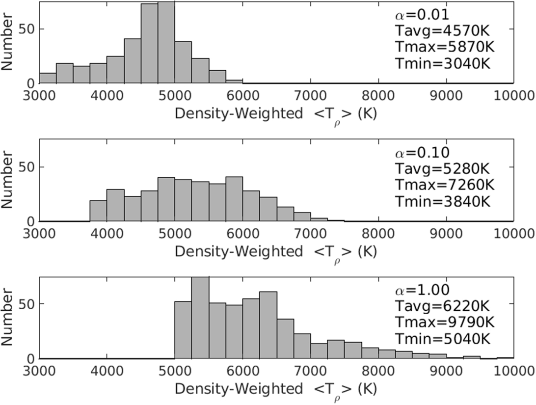
Figure 1. Histograms of the density-weighted disk temperatures (Equation (7)) for all spectral types of Table 1 and disk parameters of Table 2 resulting in detectable Hα emission. The panels are for different amounts of shear heating, controlled by the α parameter: α = 0.01 (top), α = 0.10 (middle), and α = 1.00 (bottom).
Download figure:
Standard image High-resolution imageFigure 2 plots 〈Tρ〉 versus the central stellar Teff, showing the behavior at different spectral types. Unlike the previous figure, Figure 2 shows 〈Tρ〉 for all computed models, not just those that show Hα emission. Models that satisfy the requirement of Hα emission are shown as large symbols (color coded by the choice of α), whereas models that do not show Hα emission, and would not be classified as CAe stars, are shown as small dots. There are several points of interest in this figure. First, the segregation of models by the amount of shear heating (controlled by the α parameter) becomes noticeable around spectral type A2, and for cooler stars, the temperatures of all α = 1.00 disks with detectable Hα emission lie above the 〈Tρ 〉 = 0.6 Teff line. The 〈Tρ 〉 = 5000 K plateau seen in Figure 1 is clearly visible (red symbols). Second, the fraction of models that produce detectable Hα emission (compare large symbols with small ones) is strongly dependent on the α parameter for spectral types cooler than A2 (this is further discussed below). Third, some high 〈Tρ〉 values are present, some of which exceed the stellar Teff when shear heating is present. It is important to note, however, that such disk temperatures appear almost exclusively for models that do not exhibit Hα emission and would not be classified as CAe stars.
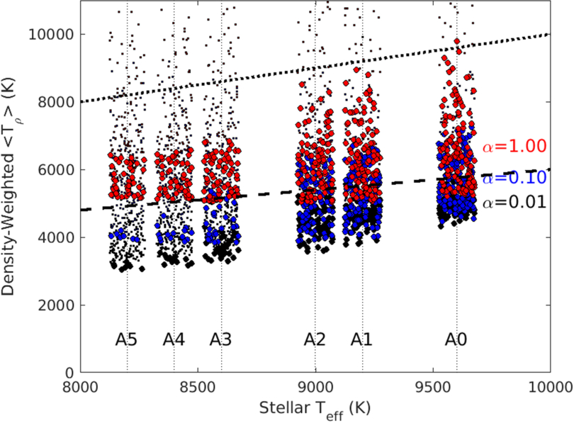
Figure 2. The density-weighted disk temperature (Equation (7)) as a function of the central star’s effective temperature. Each point represents 〈Tρ〉 (Equation (7)) for a different combination of parameters (spectral type, n, ρ0, α), with the corresponding Teff values randomly jittered by ±100 K for visibility. Symbol colors indicate different levels of shear heating governed by the viscosity parameter α: α = 0.01 (black), α = 0.10 (blue), and α = 1.00 (red). Large symbols correspond to models that produce detectable Hα emission; small symbols denote nonemitting models. The lines 〈Tρ〉 = Teff (thick dotted) and 〈Tρ〉 = 0.6Teff (thick dashed) have been added for reference. Faint, vertical dotted lines mark the Teff values corresponding to the spectral types listed in Table 1.
Download figure:
Standard image High-resolution imageModels that do not exhibit detectable Hα emission are too rarefied to have significant Hα emissivity, i.e., they have a combination of small ρ0 and/or large n in Equation (1) that leads to very low ρ(R, Z) throughout the entire disk. The gas cooling processes in the disk, namely the escape of collisionally excited line radiation, the escape of photons formed by recombination, and free–free emission, all vary with ρ2. Photoionization heating, while proportional to ρ, also requires a photon in the initial state, and the radiation energy density decreases with geometric dilution as one moves further away from the star. Shear heating, on the other hand, is proportional to ρ. For models in which shear heating becomes important, the ratio of heating-to-cooling scales as 1/ρ, and thus low-density regions have difficulty cooling, driving higher temperatures. This can dominate the temperatures in rarefied disks with small ρ0 and large n. However, these low-density disks have low emissivity and thus make little contribution to an observable diagnostic such as emission in Hα. This is the reason why we have been careful to classify all models as to whether or not they can produce emission in Hα and hence could be observed as CAe stars.
It is not clear to what extent the high disk temperatures discussed above are an artifact of assuming a constant α parameter for the entire disk volume. While molecular viscosity is independent of the gas density,9 molecular viscosity is incapable by many orders of magnitude to make viscous accretion or decretion disks viable (J. Frank et al. 2002); the viscosity in CAe and CBe stars is likely driven by turbulence and/or magnetic fields which could introduce some dependence on location in the disk (S. J. Desch et al. 1998). While this is an interesting point, we did not pursue models with ad hoc parameterizations of α, i.e., α(R, Z), as the disks affected did not present Hα emission and are not relevant to the observed samples of CAe stars discussed here.
Figure 3 shows for each Teff the percentage of star+disk models (of the 7260 computed for each spectral type and α combination) that result in detectable Hα emission for the various levels of shear heating considered as controlled by the α parameter. Note that α = 0.30 is also included in this figure. Figure 4 shows how the Hα emission fraction at each spectral type depends on α. For the earliest spectral type, A0, there is essentially no dependence of the percentage of computed models with Hα emission on α. However, this changes at spectral type A2, where shear heating can become important. By spectral type A4, there is a strong dependence of the emission fraction on α in the sense that larger α values lead to a larger fraction of models that exhibit emission; the dependence on α is essentially linear at each spectral type, as illustrated in Figure 4. In both of these figures, the absolute fraction of models with emission is somewhat arbitrary, as the set of star+disk models considered is somewhat arbitrary; for example, we could have instead retained only models that give emission at A0 and then kept this set fixed for the later spectral types, shifting the curves upward. However, the important point is that the set of models is kept the same for all spectral types so that relative changes are significant. Figures 3 and 4 strongly suggest that the fraction of Ae stars detected at the latest spectral types (A3 and A4, and potentially A5 if there are such objects) might be able to be used to constrain α through its effect on disk temperatures and Hα emission. We look at this point in Section 4.
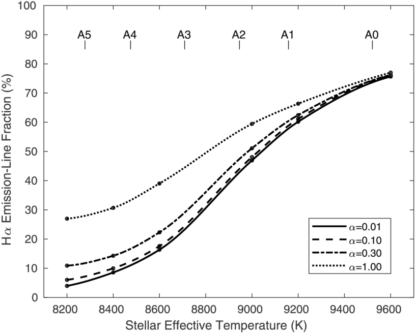
Figure 3. The fraction of computed models (Table 2) that result in detectable Hα emission as a function of the central star’s Teff. Four lines are shown corresponding to the choices for the α parameter setting the viscosity: α = 0.0 (solid), α = 0.1 (dashed), α = 0.3 (dashed–dotted), and α = 1.0 (dotted). The circles are the calculations, and the lines are spline fits to this data. The spectral type—Teff calibration is from D. F. Gray (2022) and is not rounded to the nearest 200 K as in Table 1.
Download figure:
Standard image High-resolution image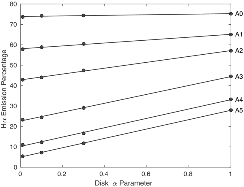
Figure 4. The dependence of the Hα emission fraction on the disk α parameter controlling the amount of shear heating. The α value associated with each line is given in the legend. The circles are the calculations (Figure 3), and the lines are linear fits to the data. The spectral type identifying each line is to the right.
Download figure:
Standard image High-resolution image4. Comparison with the LAMOST DR5 Ae Star Sample
In this section, we investigate the possibility of using the Ae star sample of R. Anusha et al. (2021) to constrain the disk α viscosity parameter appropriate to CAe star disks using both the observed variation of the fraction of detected Ae stars with spectral type and the Hα equivalent width (EW) distributions for different spectral types.
The CAe sample from R. Anusha et al. (2021) is based on the data release 5 (DR5) survey of the Large Sky Area Multi-Object Fiber Spectroscopic Telescope (LAMOST). LAMOST is operated by the Chinese Academy of Sciences (X.-Q. Cui et al. 2012), and their survey was initiated by the National Astronomical Observatories of China. R. Anusha et al. (2021) utilized the stellar spectra from LAMOST DR5 to identify and characterize CAe stars based on their Hα emission, IR color, and IR excess. This work identified 159 CAe stars that are utilized for the present study. Additionally, we crossmatched these targets with the LAMOST low and medium-resolution spectral catalogs from data release 8 (DR8), discovering 23 new observations of these stars. This makes a total of 220 potential Hα spectra for the 159 CAe stars from R. Anusha et al. (2021). For stars with multiple spectra available, we included only the single spectrum with the highest signal-to-noise ratio (S/N) in the vicinity of Hα. The mean distances of these targets, crossmatched with C. A. L. Bailer-Jones et al. (2021), range from 350 to 4900 pc, with errors increasing to up to 15% for distances greater than 3000 pc. The V-magnitudes of the targets, crossmatched with APASS DR9 (A. A. Henden et al. 2015), range from 10.0 to 16.8 mag. All targets are positioned toward the Galactic anticenter, with more than 95% of the targets located between 120∘ ≤ ℓ ≤ 240° as the LAMOST survey focuses on the Galactic anticenter.
The spectral types of the 159 CAe star sample range from A0 to A4, with the breakdown: A0 (71 objects), A1 (38 objects), A2 (35 objects), A3 (12 objects), and A4 (3) objects. No A5 or later stars were identified with Hα emission. The spectral type of each LAMOST DR5 spectrum is estimated using the LAMOST Stellar Parameter Pipeline (Y. Wu et al. 2014). However, the presence of a potentially veiled continuum and the presence of emission lines for CAe stars can complicate the spectral classification (V. Doazan et al. 1991; W. Hummel & M. Vrancken 2000). Therefore, R. Anusha et al. (2021) reestimated the spectral types semiautomatically using a template matching technique with the MILES stellar spectral library (P. Sánchez-Blázquez et al. 2006).
For each object, the Hα line was extracted and continuum normalized (at ±37 Å) in order to measure its EW. In contrast to R. Anusha et al. (2021), a photospheric Hα EW appropriate to the star’s spectral type was not subtracted from the measured EW. We adopt the convention that EW > 0 represents net emission and EW < 0, net absorption. The average S/N around the Hα lines is typically ≈90, and the renormalized spectra yielded Hα EWs ranging from −12.1 to +24.2 Å. The lines were also morphologically classified into the categories defined in Section 2.3. From the sample of 159 Ae stars, 153 (96%) were classified with an index of 121 (single emission peak in an absorption trough), two objects with an index of 12121 (doubly peaked emission in an absorption trough), and four objects with an index of 2 (single emission peak with no detectable absorption).
Figure 5 shows the distributions of measured Hα EWs as a function of spectral type. The steep decline in detected Ae stars for later spectral types, A3 and A4, is apparent. With Hα distributions for five spectral types, we performed 10 two-sample Kolmogorov–Smirnov (KS) tests, one for each pair of spectral types, to see if the distribution pairs are consistent with the same underlying distribution. The KS test is used because an unbinned test is desirable, given the small number of objects with A3 and A4 spectral types. The results are presented in Table 3, which gives, for each pair of spectral types, the  of the probability (
 ) that a KS statistic equal to or larger than observed is consistent with random sampling of the same underlying distribution. At the 1% level, no comparisons fail. At the 5% level (
 ) only the A1–A2 comparison fails. The interpretation of this failure is not entirely clear. Given the results of the calculations in Section 3, one might have expected failures between earlier (A0 and A1) and later (A3 and A4) spectral types; however, the very small number of objects at A3 and A4 precludes sensitive tests.
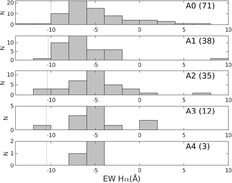
Figure 5. Histograms of the measured LAMOST Hα equivalent widths (in Ångstroms) for each spectral type in the Ae star sample of R. Anusha et al. (2021). The number of sample stars for each spectral type is given in brackets. EW< 0 is net absorption, whereas EW> 0 is net emission. The dotted line in each panel gives the LTE, photospheric absorption Hα equivalent width for  at that spectral type.
Download figure:
Standard image High-resolution imageTable 3. Two-sample KS Tests for Each Pair of Equivalent Width Distributions Shown in Figure 5
| Spectral Type | A0 | A1 | A2 | A3 | A4 |
|---|---|---|---|---|---|
| A0 | 0.000 | −0.991 | −0.124 | −0.123 | −0.112 |
| A1 | 0.000 | −1.645 | −0.975 | −0.260 | |
| A2 | 0.000 | −0.176 | −0.025 | ||
| A3 | 0.000 | −0.051 | |||
| A4 | 0.000 |
Note. Each entry gives the  of the probability that the equivalent width distributions of the spectral types in the row and column headers are drawn from the same underlying distribution.
Download table as: ASCIITypeset image
The small number of objects of spectral types A3 and A4 does make the analysis to follow sensitive to the possibility of spectral type misclassification, i.e., these objects might be misclassified as earlier spectral types. For this reason, we have visually recompared the spectra for the A3 and A4 objects with the available MILES templates. Figure 6 compares two of the CAe stars (spectral type A4: LAMOST J114805.60+412843.2, and spectral type A3: LAMOST J184640.36+425427.9) to the A1V template in the vicinity of 4000 Å. Noteworthy is the Ca ii K line at λ3934. This line is very temperature sensitive over the range of the A stars, with its strength increasing with decreasing Teff. As can be seen from the figure, the Ca ii K line in the A4 and A3 spectrum is much stronger than in the A1 template. The other comparisons gave similar results, and there is no clear evidence that the A3 or A4 spectral types are misclassifications.
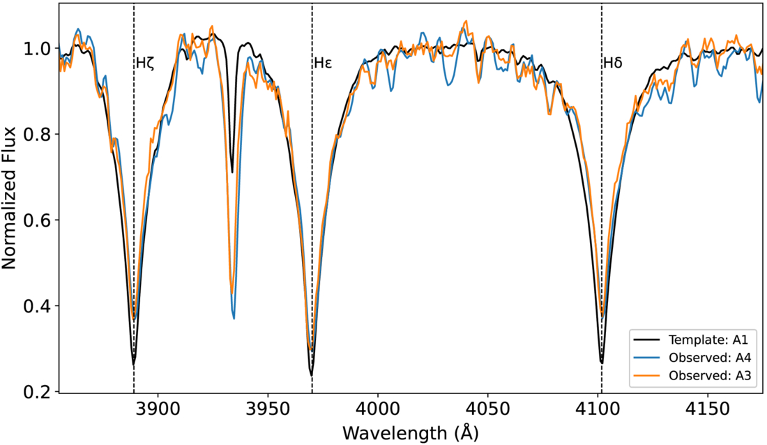
Figure 6. Comparison of the optical spectrum of a LAMOST A4-type CAe star (blue line, LAMOST J114805.60+412843.2) and an A3-type CAe star (orange line, LAMOST J184640.36+425427.9) with the A1-type MILES template (black line). Note the mismatches in the central depths of the hydrogen series Hζ, H, and Hδ, as well as in the strength of the Caii K line at λ3934.
Download figure:
Standard image High-resolution image4.1. Fraction of Ae Stars with Spectral Type
In this section, we will test if our CAe star Hα calculations above are consistent with the steep decline in the number of CAe stars with spectral type detected by the LAMOST sample of R. Anusha et al. (2021).
Consider a sample of N stars. The number of stars of class c1 in this sample that have detectable Hα disk emission can be written as

Here fc1 is the fraction of sample stars that are of class c1, Dc1 is the fraction of such stars that have disks, and Ec1 is the fraction of disks that result in detectable Hα emission. Given some other class c2, the ratio of the number of stars with detectable Hα disk emission in class c2 to those in class c1 is

In this expression, the ratio fc2/fc1 can be obtained directly from the survey. The ratio Dc2/Dc1 could be in general complex, but in the present case of A-type main-sequence stars over a limited range of adjacent spectral types, it does not seem unjustified to assume that Dc2/Dc1 ≈ 1. The third ratio, Ec2/Ec1, can be deduced from Figure 4. To apply this to the LAMOST sample, we take class c2 to be spectral types A3 and A4, and class c1 to be spectral types A0 and A1; we have combined spectral types in this manner for several reasons. First, combining A3 and A4 increases the number of objects in the cool bin. Second, the reason for the large difference in the number of A0 and A1 stars (over a factor of 2) is not entirely clear to us.10 Finally, these two combined bins straddle where the steep decline starts in Hα emission numbers.
From the spectral type counts of the LAMOST DR5 sample, N(A34) = 76087 and N(A01) = 89036; therefore, fA34/fA01 ≈ 0.86.11
R. Anusha et al. (2021) find  (Figure 5). Figure 4 suggests EA01 ≈ 0.7. Putting this together, we can solve Equation (9) for EA34 to find
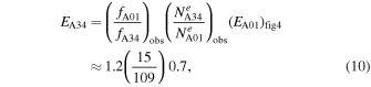
or EA34 ≈ 12% which is consistent with Figure 4 with α ≤ 0.1. This agreement might be somewhat fortuitous given the uncertainties. If we assume the error is dominated by the  uncertainty in the A3/A4 counts, the 1σ range of EA34 is approximately 8%–15%; therefore, the result is not statistically inconsistent at 2σ with α ≤ 0.30. In addition, this result is based on the assumption that Dc2/Dc1 ≈ 1 (that similar disks occur for both early- and late-type CAe stars), which might not be true. Nevertheless, our Hα calculations seem consistent with the steep decline in CAe star numbers at essentially the correct A2 spectral type.
4.2. Modeling the LAMOST Equivalent Width Distributions
A stricter comparison with the CAe star sample of R. Anusha et al. (2021) is to compare the range of Hα emission strengths, as opposed to the binary “Yes/No” emission classification of Section 4.1, using CAe star counts. In this section, we attempt to match the observed Hα EW distributions for each spectral type shown in Figure 5. In practical terms, the cumulative distribution (CDF) of the observed Hα EWs will be compared with samples constructed from the models of Section 2.3 using a two-sample KS test in order to avoid binning the observed data.
We use the Hα calculations of Section 2 to build CAe samples of 100 stars for each spectral type and viscous α value that can then be compared to the observed samples in Figure 5. To do this, we need to specify probability distributions for the disk density parameters (ρ0, n, Rd), as well as the viewing inclination angle i, as these are required to fully specify each model Hα profile.12
The viewing inclination angle distribution is straightforward: for randomly oriented stellar rotation axes, the inclination angle i follows the  distribution for the observer (D. F. Gray 2022). The distributions for (ρ0, n) are less straightforward, but it is reasonable to model these distributions as Gaussians13
specified by a mean and standard deviation (see, for example, T. A. A. Sigut & N. R. Ghafourian 2023). Thus to build random samples of calculated Hα profiles, we generate the inclination angle i from the
distribution for the observer (D. F. Gray 2022). The distributions for (ρ0, n) are less straightforward, but it is reasonable to model these distributions as Gaussians13
specified by a mean and standard deviation (see, for example, T. A. A. Sigut & N. R. Ghafourian 2023). Thus to build random samples of calculated Hα profiles, we generate the inclination angle i from the  distribution and generate (ρ0, n) from

and

Here (μρ, σρ) are the mean and standard deviation for the  distribution, (μn, σn) are the mean and standard deviation for the n distribution, and rN(0, 1) and
  are normally distributed random numbers with a mean of zero and a standard deviation of one. We take the outer disk radius, Rd, to be uniformly distributed between 5 and 50 R*, i.e.,

where r is a uniform deviate, 0 ≤ r ≤ 1.
To fit an observed distribution of Hα EWs for a specific spectral type, we follow the above procedure to generate a random sample of 100 computed Hα profiles for models with a selected viscous α parameter and compare the CDF of the model Hα EWs to the observations. The random sample includes only models where the Hα profile is classified as having an emission component in order to match the selection procedure for the observed sample (i.e., selection for CAe stars). The comparison is a two-sample KS test with the goodness-of-fit parameter taken as the probability that one would obtain a KS test statistic (maximum difference between the CDFs) equal to or larger than observed (J. V. W. Wall & C. R. J. Jenkins 2003). As the inclination angle (i) and outer disk radius (Rd) distributions are fixed, this comparison is repeated over the 1512 combinations of the (μρ, nρ; μn, σn) values listed in Table 4 in order to maximize this probability and define the best-fit model. These values are chosen to span the known range of disk density parameters for the CBe stars. It is important to note that our goal is not to extract good measures of these parameters from the data; our real interest is if there is a consistent set of parameters that can reproduce the data for each α viscosity parameter considered.
Table 4. Mean and Standard Deviation Parameters Used for the Distributions of  and n
and n
| Parameter | Values |
|---|---|
| μρ | (6): −11.50, −11.25, −11.00, −10.75, −10.50, −10.25 |
| σρ | (6): 0.10, 0.20, 0.40, 0.60, 0.80, 1.00 |
| μn | (7): 2.00, 2.25, 2.50, 2.75, 3.00, 3.25, 3.50 |
| σn | (6): 0.10, 0.20, 0.40, 0.60, 0.80, 1.00 |
Download table as: ASCIITypeset image
Given this procedure, there are several options as to how to proceed: (1) adopt  values derived for the Be stars (use, for example, T. A. A. Sigut & N. R. Ghafourian 2023); (2) fit the A0 spectral type, for which there is essentially no dependence of the Hα distribution on α, and then use the obtained best
  values to generate the samples for the remaining spectral types, A1 through A4, and α values; (3) fit individual (μρ, nρ; μn, σn) parameters to the observed Hα distribution for each spectral type and α value, and then search for consistency in these parameters across the spectral types.
After some trial and error, we have adopted approach (3). The reasoning here is twofold: first, adopting distributions appropriate for the Be stars, such as those of J. Silaj et al. (2010) or T. A. A. Sigut & N. R. Ghafourian (2023), would include the influence of many high-mass Be stars, which are much different than the cool Ae stars considered here. Even within the CBe stars, there is evidence of different disk parameters between high and low mass CBe stars (C. Arcos et al. 2017). Second, fixing the distribution to that found for the A0 stars (or the Be stars as in option 1) does not work well in practice. The best-fit disk density model for the A0 stars fails to reproduce the Hα CDFs for the cooler spectral types. However, this is not an inconsistency because, in practice, a large number of distributions will fit the observed data nearly as well as the best-fit model; therefore, one ends up in searching over a large number of parameter combinations for consistency, and this begins to look like option (3) in the end.
The result of this procedure is shown in Figure 7. For each combination of spectral type, A0 through A4, and α parameter, α = 0.10, 0.30, and 1.00, the observed Hα EW CDF of Figure 5 is compared to the various model CDFs as defined by (μρ, nρ; μn, σn). The best-fit model CDF is shown, as well as all models that fit at the 5% level or better, based on the two-sample KS test. As can be seen from the figure, good fits to the observed Hα CDFs can be obtained for the A0 and A1 spectral types, and there is little dependence of these theoretical CDFs on the α parameter used. The best-fit parameters (μρ, nρ; μn, σn) are discussed below.
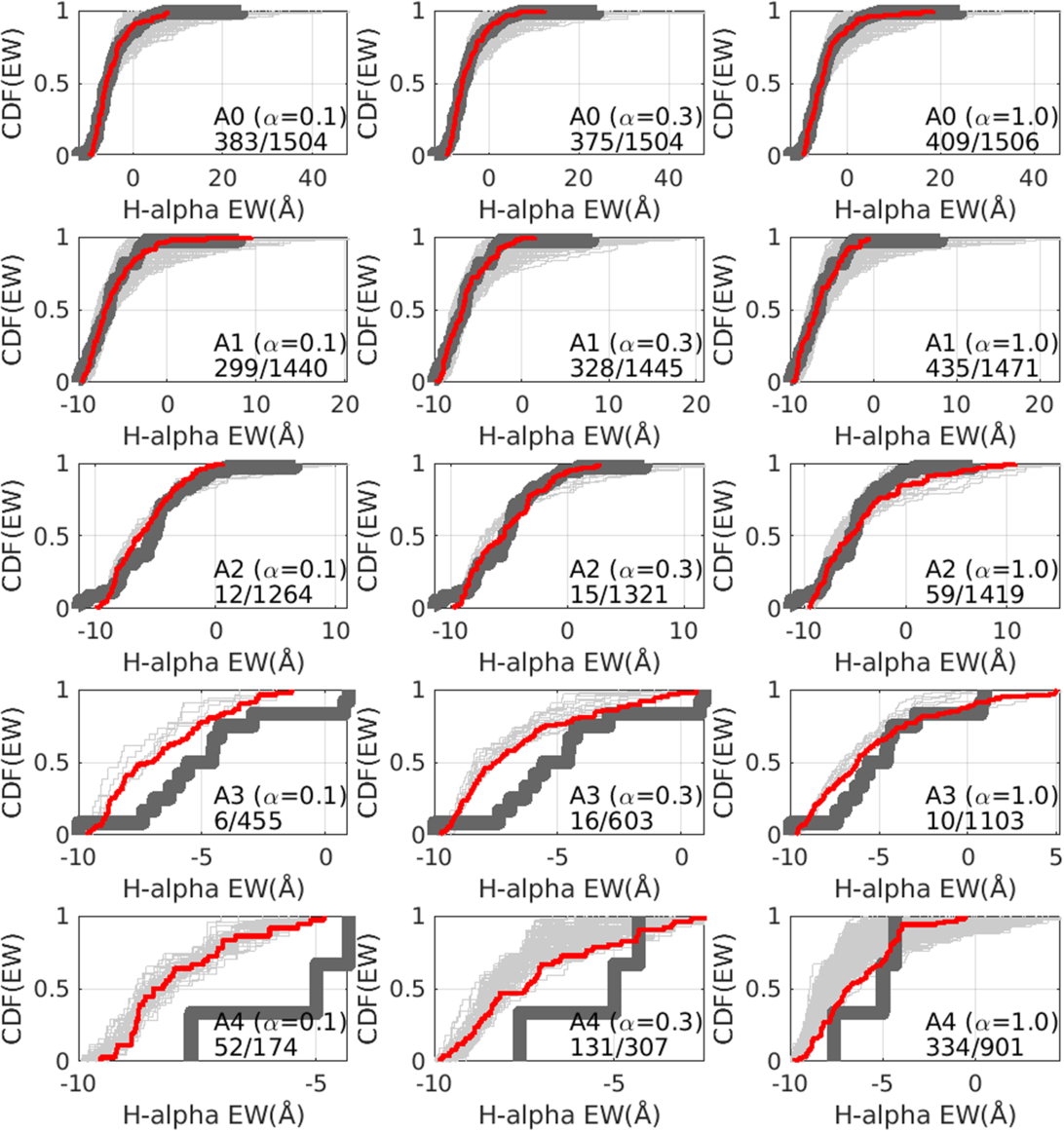
Figure 7. Best model fits to the CDF of the observed Hα EWs shown in Figure 5. The five rows correspond to spectral types A0 through A4 (top to bottom), and the three columns correspond to three α values controlling the amount of shear heating: α = 0.1 (left), 0.3 (middle), and 1.0 (right). The wide, dark gray line in each panel is the observed Hα CDF (and is the same across each row). The red line is the Hα CDF for the best-fit computational sample, and the light gray lines are all computed samples that satisfy  (5% level). The number of such samples, out of the total number of samples checked, is also shown in each panel.
Download figure:
Standard image High-resolution imageThere is an interesting trend in the fits with spectral type shown in Figure 7. Each panel also gives, for that spectral type and α, the number of models out of the number tested that fit with a two-sample KS probability of 5% or higher.14 For spectral types A0 and A1, several hundred of the parameter combinations of Table 2 fit at least at the 5% level, with the α = 1.00 models having slightly more fits. However, this changes for spectral types A2 and A3. The number of fitting models is now down to the single digits for α ≤ 0.3, whereas tens of models fit for α = 1.00. Recall that A2 is where shear heating first becomes important. At A4, the number of fits rises again, with the most for α = 1.0, but this is really a consequence of having an observational sample size of just three.
What about the consistency of these fits, i.e., can all of the CAe Hα observations be modeled with a single choice for μρ and μn, i.e., a single choice for the distributions of disk density parameters? This is addressed in Figure 8, which plots, for the α = 1.00, the model samples that fit to 5% or better in the (μρ, μn) plane. Here a point is placed at the point (μρ, μn) if the Hα EW CDF of a model sample with these parameters fits the observed CDF to 5% or better (color coded by spectral type). There can be many points at a single (μρ, μn) because there are many choices for the additional (σρ, σn) parameters; these are jittered for clarity. As can be seen from the figure, wide portions of the parameter space are consistent with the A0 and A1 Hα strengths, due to the intrinsically stronger Hα emission, and the A4 Hα strengths, due to the small observed sample not providing a strong constraint. The real test is the intermediate A2 and A3 spectral types where the Hα strengths are rapidly falling, the influence of shear heating is increasing, and the sample sizes are large enough to provide meaningful constraints. For α = 1.0, there is a small portion of the parameter space spanned by Table 2 where all spectral types, A0 through A4, can be fit, and this region occurs in the upper left corner of the figure, where (μρ, μn) ∼ (−10.50, 2.00). For the other α values, α ≤ 0.3 (not shown in the figure), no such common region can be found.
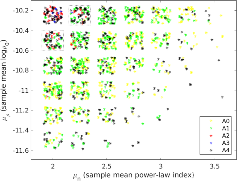
Figure 8. Parameters (μρ, μn) for the theoretical Hα CDFs fits of Figure 7 corresponding to the rightmost column of Figure 7 for α = 1.0. All models have KS probabilities  . The symbols are color coded by spectral type as identified in the legend. Corresponding to each (μρ, μn) are a number of CDFs corresponding to different choices for (σρ, σn) (see Table 4). These models are randomly jittered about their common (μρ, μn) values for clarity. The two dotted squares in the upper left corner mark consistent samples for which all five spectral types occur for the same (μρ, μn).
Download figure:
Standard image High-resolution imageWe do not want to overinterpret this result. This method is not a sensitive way to determine the underlying  distributions for a sample of stars, as clearly demonstrated by the large number of fits at spectral types A0 and A1. However, there is a hint in the analysis that the strengths of the Hα line, particularly for A3 and A4 (where shear heating has been theoretically demonstrated to be important) are not consistent with α ≤ ≈0.3. This is, of course, contrary to the previous discussion focused on CAe star counts, and apparently inconsistent with the absence of CAe stars of spectral type A5 or later (see Figure 2). More sensitive searches for weak Hα emission at spectral types A3 and later would be very helpful in clarifying this situation.
5. Conclusions and Future Work
We have constructed theoretical models for the temperature structure of circumstellar disks surrounding A-type main-sequence stars that include both radiative heating from the central star and viscous shear heating from the disk’s Keplerian rotation, with the viscosity modeled by the α prescription of N. I. Shakura & R. A. Sunyaev (1973). For spectral types A0 and A1, the contribution of shear heating, even with α = 1.0, is small and makes no significant impact on the predicted disk temperatures or Hα emission-line strengths. However, for spectral type A2 and cooler, shear heating can become significant, and the choice of α affects the strength of the Hα emission. In particular, shear heating with α ≥ ∼0.3 can prevent CAe star disks from becoming as cool as predicted by the trend for average disk temperatures of ∼0.6 Teff based on radiative heating alone. All models show a significant decline in the number of CAe stars near spectral type A2 based on calculated Hα emission; however, this decline is moderated by increasing α. Models with α = 1.0 also predict significant emission for spectral type A5, although no such objects have been observed.
The dependence of the presence and strength of Hα emission on shear heating for latter spectral types makes it possible to constrain the disk viscosity α parameter using observed samples of CAe stars, both in terms of number of classified CAe stars as a function of spectral type and on the strength and distribution of the Hα emission EW. This radiative method is a novel approach for CAe stars, as previous measurements of α in CBe circumstellar disks have relied on hydrodynamical modeling with the implied viscous timescale, t ∼ R2/ν, to match observed variations of disk emission. However, this radiative method is limited to providing some sort of “ensemble average” of α over the CAe population, as opposed to being extracted for individual objects. If the underlying physical process for the viscosity is, for example, magnetic fields via the magnetorotational instability (S. A. Balbus & J. F. Hawley 1991), variations in the magnetic field strength and/or geometry might give rise to variations in α between objects, something this radiative approach cannot capture. Nevertheless, given the central role viscosity plays in the circumstellar disks of CAe and CBe stars, all constraints are valuable.
We have attempted to extract such an ensemble-averaged α for the CAe sample of R. Anusha et al. (2021). The results are not consistent. The drop in the fraction of CAe stars as a function of spectral type in the range A0 through A4 seems most consistent with α ≤ ≈0.1, although there are large uncertainties as the number of A3 and A4 stars in the sample is small. On the other hand, modeling the observed Hα emission-line strength as a function of spectral type through the CDF of the Hα EW suggests that α is larger, with the evidence coming from spectral types A3 and A4; however, the number of detected objects for these later spectral types is small. In addition, α = 1.0 models lead to the expectation of spectral type A5 CAe stars (see Figure 2), yet none are seen. This disagreement in α for CAe counts versus Hα EW CDF is likely due to the statistics of small numbers, and steady improvements will be realized as the number of CAe stars, particularly for the latest spectral types, increases.
As a follow-up to this study, we plan to match all the available Hα spectra for the 159 CAe stars in the R. Anusha et al. (2021) sample using the Bedisk/Beray code suite to obtain best-fit disk density parameters (ρ0, n, Rd) and inclination angles for each individual star. This will allow a detailed comparison with the known distributions for the CBe stars of J. Silaj et al. (2010) and T. A. A. Sigut & N. R. Ghafourian (2023).
A final point we have not addressed in this work is the potential role of A shell stars, where Hα emission is not detected, but deep central absorption well below the expected photospheric profile is seen. Such objects are a natural extension of the CAe stars in which the inclination of the system is high, i ≥ ≈80°, in which the observer’s line of sight passes directly through the thin, equatorial disk. Hα shell stars are known to extend to later spectral types than the CAe stars, predominantly seen to spectral type A5, with a decline toward A7 and near disappearance after that (A. Slettebak 1982; R. W. Hanuschik 1996; B. Hauck & C. Jaschek 2000). The Hα calculations in this work also naturally predict the frequency and absorption strength of the Hα shell feature as a function of spectral type, and we will examine this line of reasoning in a subsequent work.
Acknowledgments
The authors are grateful to the anonymous reviewer for their constructive feedback and careful reading of the manuscript, which helped enhance both the clarity and quality of our work. T.A.A.S. gratefully acknowledges funding from the Natural Sciences and Engineering Research Council of Canada (NSERC) through the Discovery Grant program.
Footnotes
- 3
The rotation speed at which the effective gravitational acceleration at the equator vanishes.
- 4
R is the distance from the stellar rotation axis, and Z is the height above (Z > 0) or below (Z < 0) the equatorial plane.
- 5
This gives γ = 1.333, which lies between isothermal (γ = 1) and adiabatic (γ = 5/3) motion for the turbulent eddies that underlie the viscosity.
- 6
While we have assumed α to be constant over the entire disk, variations of α with R and/or Z are certainly possible (see also A. Granada et al. 2021).
- 7
This resolution is chosen to closely match the observed sample discussed in Section 4.
- 8
It might seem contradictory that such cool disks could produce any Hα emission at all. However, 〈Tρ〉 is just an average for the disk. In reality, there are usually strong temperature variations in photoionized disks, particularly in the vertical (Z) direction. Such disks typically have hot sheaths above and below the equatorial plane that are directly illuminated by the star, with cooler regions near the equatorial plane where the star’s radiation suffers significant extinction due to high optical depths along all rays back to the star—see, for example, T. A. A. Sigut & C. E. Jones (2007).
- 9
A fact that surprised Maxwell when he derived this result in 1860 (W. G. Vincenti & C. H. Kruger 1965).
- 10
This may have to do with the availability (or lack thereof) of A spectral subtype templates used in the classifications.
- 11
Based on the Salpeter IMF and crudely assigning c1 (A0–A1) to mass bin [2.30, 2.50] M⊙ and c2 (A3–A4) to mass bin [2.00, 2.20] M⊙ solar masses, one might have expected the ratio fc2/fc1 ≈ 1.4.
- 12
The parameter ranges in Table 2 simply define a computational grid of models, and there is no guarantee that every model is realized by an actual star. In addition, some parameter combinations do not result in Hα emission and hence fail the requirement for a CAe star.
- 13
Technically the distribution for ρ0 is lognormal as
 is taken to be normally distributed.
 - 14
From Table 2, there are a maximum of 1512 models, but it provided difficult to build random samples of 100 stars with Hα emission for some choices of the parameters (μρ, nρ; μn, σn), particularly for later spectral types (A3 and A4) with little shear heating (i.e., small α). Only parameters that could furnish samples of 20 or more (out of 200 attempts) were retained in the comparison.
