Abstract
In this study, we develop deep learning models to forecast the 6 hr interplanetary magnetic field (IMF) Bz component for southward cases. The models are based on a bidirectional long short-term memory method, and input parameters are solar wind data (V, N, T) and IMF components (Bt, Bx, By, Bz). The data are obtained from OMNI, whose period is from 2000 to 2022. We use the preceding 12 hr of data as input and the subsequent 6 hr of Bz data as target. To focus on strong geomagnetic conditions, we consider periods where Bz values drop below the negative standard deviation (approximately −3 nT) for at least 6 hr. The models are trained and validated using a 12-fold cross-validation process, with each model trained over 8 months of data and tested over 4 months. The ensemble model, which averages 12-fold model results, achieves an RMSE ranging from 1.75 (30 minutes prediction) to 2.55 nT (6 hr prediction), significantly outperforming two baseline methods: multilayer perceptron and multiple linear regression. Our model can capture both decreasing and increasing phases of Bz, showing reliable performance across varying geomagnetic conditions. Our results suggest a sufficient possibility for predicting Bz under noticeable southward conditions. We expect that our model can be used for subsequent space weather predictions, such as global magnetohydrodynamic simulations in the magnetosphere.
Original content from this work may be used under the terms of the Creative Commons Attribution 4.0 licence. Any further distribution of this work must maintain attribution to the author(s) and the title of the work, journal citation and DOI.
1. Introduction
Interplanetary magnetic field (IMF) refers to the Sun’s magnetic field carried by the solar wind into the interplanetary space within the solar system. Among its components, the southward component of the IMF, denoted as Bz, plays a crucial role in space weather phenomena near the Earth. It determines how much energy from the solar wind is transferred to the Earth’s magnetosphere through magnetic reconnection (J. W. Dungey 1961; R. L. Arnoldy 1971). This process is closely associated with geomagnetic storms, which can significantly affect satellites, navigation systems, communication networks, and power grids on Earth. Therefore, accurately predicting Bz is essential for space weather alerts. However, despite its importance, predicting of the IMF Bz near Earth remains a challenge due to the highly complex nature of solar winds.
Historically, various approaches have been employed to address the problem of Bz prediction. Physical and empirical models, which utilized statistical correlations between solar wind parameters and geomagnetic activity indices, have been widely used, mainly for Bz directions (J. Chen et al. 1996; N. P. Savani et al. 2015; D. Shiota & R. Kataoka 2016; C. Möstl et al. 2017). For example, X. Zhao & J. T. Hoeksema (1995) developed a method using the Current Sheet Source Surface model to extrapolate magnetic fields from the solar surface to Earth, allowing for a basic forecast of the IMF components, including Bz. In recent years, advanced data-driven and machine learning techniques have significantly improved Bz forecasting (P. Riley et al. 2017; B. Jackson et al. 2019). For instance, M. A. Reiss et al. (2021) explored the use of machine learning models trained on in situ measurements to predict the minimum Bz component for a certain period and the maximum Bt values embedded within interplanetary coronal mass ejections. To our knowledge, there has been no study to forecast the Bz profile.
Deep learning, a branch of machine learning, excels at solving nonlinear problems by utilizing multiple layers of neural networks. Due to its ability to model complex nonlinear relationships, deep learning has been increasingly applied to space weather prediction tasks (Y.-J. Moon et al. 2022, and references therein). These approaches demonstrate potential for improving prediction accuracy, particularly in time series forecasting.
Our preliminary investigation on the forecasting of Bz profiles for several days shows that is so challenging, mostly impossible. Thus we focus on the short-term forecasting of Bz components for only noticeable southward cases, i.e., when Bz falls below a certain threshold of approximately −3 nT, about the standard deviation of Bz in our data set. Our goal is to explore the feasibility of using deep learning to predict Bz during these critical periods.
This study represents the first attempt to forecast the profiles of Bz. We choose a prediction target of 30 minute intervals over a 6 hr period due to the following reasons. In global magnetohydrodynamic (MHD) models in the magnetosphere, solar wind data with high time resolution, typically covering several hours, are used as inputs (J. Lyon et al. 2004; G. Tóth et al. 2005). As we plan to use the output of our model as the input of global MHD model, it is necessary to align our approach with this requirement. Predicting the BZ profiles over longer periods is challenging due to the increasing complexity of changes in IMF Bz. Similarly, higher time resolutions tend to introduce much more fluctuations, making accurate predictions more difficult. Therefore, we select a 6 hr prediction window with a 30 minute time resolution, which is empirically determined by several trials.
This paper is organized as follows: In Sections 2 and 3, we describe the data and methodology used, respectively. In Section 4, we present the results of our model and discuss them. Finally, a brief summary and conclusion are given in Section 5.
2. Data
We obtain the solar wind and IMF data from OMNIWeb (https://omniweb.gsfc.nasa.gov/), which provides time-shifted data to the Earth’s bow shock nose, based on in situ measurements from Lagrangian point 1 satellites. Our model uses solar wind speed (V), density (N), temperature (T), IMF strength (∣B∣), and the components of the IMF (Bx, By, and Bz). These parameters serve as input data, structured into sequences of 24 time points, corresponding to 12 hr of measurements averaged over 30 minute intervals. The target data consist of the IMF Bz for the next 6 hr, averaged over 30 minute intervals. The IMF components are expressed in geocentric solar magnetospheric (GSM) coordinates, as IMF Bz in GSM coordinates is known to be strongly associated with geomagnetic storms (W. D. Gonzalez & B. T. Tsurutani 1987). The total period of the data we use is from 2000 to 2022.
Based on our preliminary investigation and other studies, we realize that predicting all Bz values is challenging due to the natural tendency of Bz to converge toward an average of zero. This tendency causes deep learning models to similarly converge their predictions toward zero. This makes it difficult for the model to accurately predict strong southward components, which are of particular interest. To address this issue, we employ a new strategy, focusing on cases where Bz values drop below a specific threshold, defined as the negative standard deviation (–std) of Bz, approximately −3 nT. This threshold is determined as a reasonable compromise to balance the availability of the number of data and the need to focus on significant geomagnetic conditions.
Figure 1 illustrates the methodology used to construct the data set. We consider cases where the IMF Bz remains below –std for at least 6 hr. These periods are segmented into 6 hr intervals, which are used as target data for our model. Each dashed box in Figure 1 represents one such segment of the target data. The sliding window approach is applied to shift these 6 hr segments forward in time with a 30 minute window. For example, if the event starts at 00:00 and lasts 8 hr, the data set will include overlapping intervals such as 00:00–06:00, 00:30–06:30, and 01:00–07:00, etc. This process results in a total of 4360 data pairs. While some overlap exists between adjacent 6 hr intervals, each interval represents a unique temporal context. For example, the intervals 00:00–06:00 and 00:30–06:30 contain some common data points, but they represent different temporal patterns. Although individual data points may appear in multiple intervals, the focus of the models is on learning the temporal dynamics rather than memorizing individual values. Thus, overlapping data points do not compromise the independence of each interval as the model perceives them as separate samples. This sliding window approach has been widely employed by several time series forecasting studies (K. Yi et al. 2020; A. Ji & B. Aydin 2023; X. Sun et al. 2024).
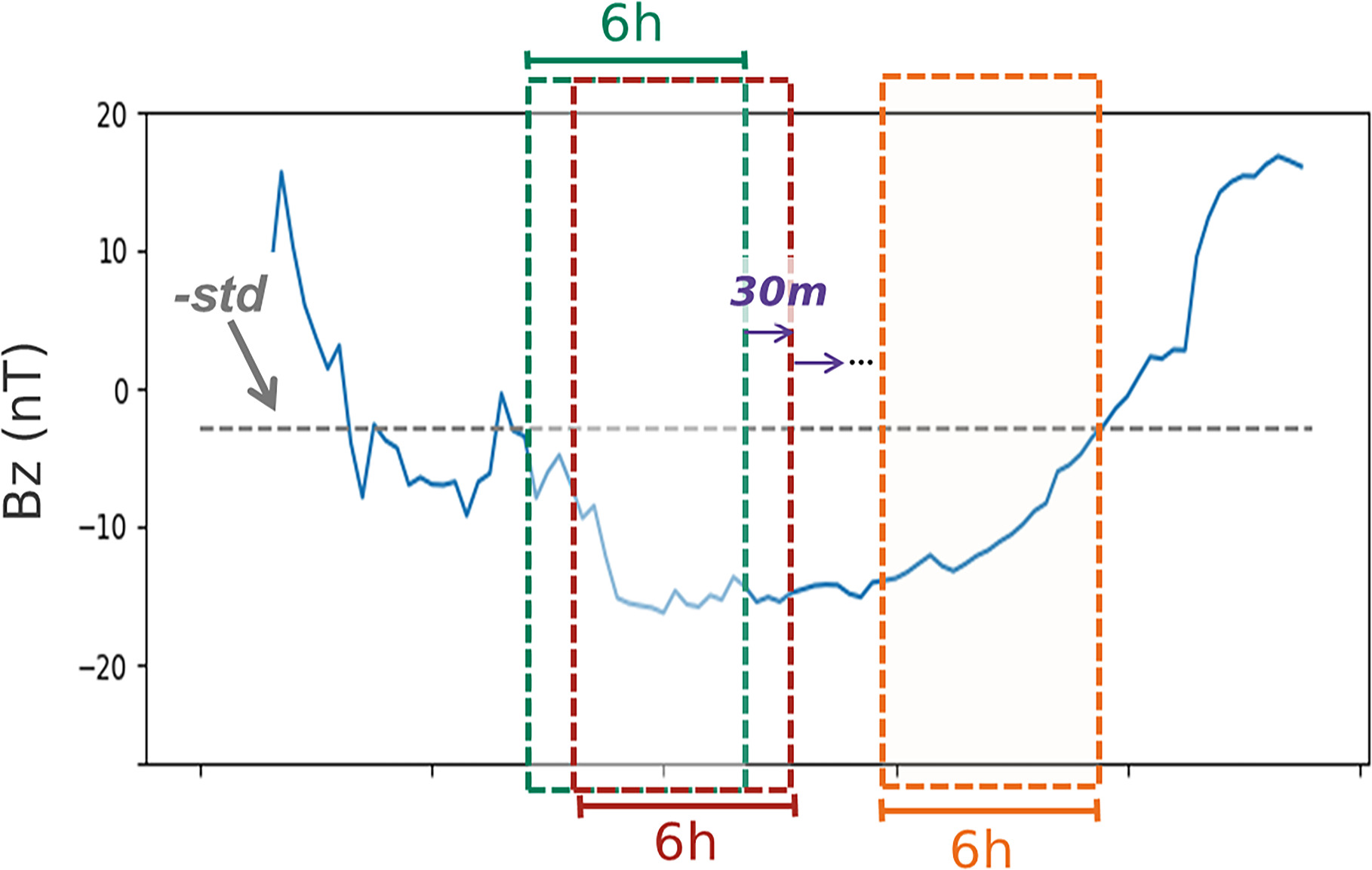
Figure 1. Method for constructing the data set. The periods where Bz remains below –std for at least 6 hr are identified. These periods are segmented into 6 hr intervals, represented by the dashed boxes, which serve as the target data. The sliding window approach is employed to shift these segments forward in time with a 30 minute window.
Download figure:
Standard image High-resolution image3. Methodology
3.1. Deep Learning Model
The long short-term memory (LSTM) network (S. Hochreiter & J. Schmidhuber 1997) was designed to address the issue of long-term dependencies that conventional recurrent neural networks (RNNs) face. LSTM networks are widely used in tasks such as language translation, speech recognition, and time series prediction. It has also been employed for space weather prediction tasks by several studies (Y. Tan et al. 2018; K. Yi et al. 2020; H. Zhang et al. 2022). However, both simple RNNs and LSTMs have a limitation: they tend to produce results that are heavily influenced by prior patterns, as they process input sequentially. To overcome this limitation, A. Graves & J. Schmidhuber (2005) suggested bidirectional LSTM (BiLSTM). A BiLSTM network consists of two LSTM layers, one processing the input sequence in the forward direction and the other in the backward direction. This bidirectional processing enables the model to better capture the contextual information in the data. BiLSTM networks have demonstrated improved performance across various tasks by capturing dependencies from both past and future contexts (A. Graves et al. 2013; A. Hu & K. Zhang 2018). In our examinations, the results of BiLSTM are much better than LSTM for our study.
In this study, we implement a model with two consecutive BiLSTM layers. Each BiLSTM layer consists of 128 hidden units and is followed by a rectified linear unit activation function (V. Nair & G. E. Hinton 2010), as shown in Figure 2. The input data of our model consist of sequences with a length of 24 and 7 features, and the output layer produces predicted Bz values for the next 12 time steps, corresponding to the next 6 hr with a 30 minutes cadence. The model has a total of 536,588 trainable parameters. For training, we utilize the Adam (D. P. Kingma & J. Ba 2014) optimizer with a learning rate 0.0001 and a batch size of 32. The loss function used is the mean squared error (MSE), which minimizes the average squared difference between the predicted and observed values. Although the model has a high parameter-to-data ratio, we carefully monitor the training and validation loss throughout the training process, and no significant increase in validation loss is observed. This indicates that the model has converged without overfitting. In addition, the models are trained for 100 epochs without early stopping. Since validation loss remains stable after an initial decrease, we conclude that continuing training 100 epochs is appropriate for optimal performance. To further validate this choice, we conduct additional training up to 600 epochs. Our results show that further training does not lead to noticeable improvements in model performance, confirming that 100 epochs are appropriate for achieving convergence. Nonetheless, we acknowledge that implementing an adaptive early stopping strategy could provide a more systematic approach to determining the optimal stopping point and further optimize the training process. To further enhance the robustness of the models, incorporating dropout and other regularization techniques could be considered in future work. The model code will be available in our GitHub repository (https://github.com/Jihyeon-ing/Bz_prediction).
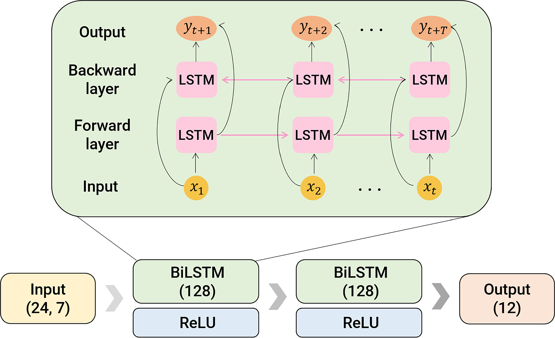
Figure 2. Model architecture used in this study. The parentheses indicate the number of nodes of each layer.
Download figure:
Standard image High-resolution image3.2. K-fold Validation
Due to the insufficient data sets for training the deep learning model, we employ the K-fold validation method. K-fold validation is a technique that divides the data set into K parts (or “folds”). For each iteration of training, one of the K folds is used as the test set, while the remaining folds are used as the training set. This process is repeated K times, with each fold being used exactly once as the test set. This method not only maximizes the use of available data but also helps to reduce the risk of overfitting and ensures that the model is robust and generalizes well.
Taking into solar cycle effects, we divide the entire data set as follows: 8 months of data for training and the remaining 4 months for testing. Additionally, the last 10% of the training set are further separated as the validation set to monitor the model’s performance model during training. For example, in the first fold, data from January to August of each year are used as the training set, with the last 10% of this data designated as validation set. The remaining data from September to December of each year are used as the test set. In the subsequent fold, the split shifts forward by 1 month: the training set consists of data from February to September of every year, and the test set includes data from October to January of every year. This process is repeated across 12 folds. Consequently, we train 12 independent models, each corresponding to a different fold in the K-fold cross-validation process. In each iteration, each of these models is trained and tested independently on different data splits. The final performance is evaluated by aggregating the results from all 12 models. This repeated training ensures that our model is tested against a variety of data splits, thereby enhancing its reliability and accuracy. To guarantee robust model evaluation and avoid data leakage, we further employ a monthly data exclusion and ensemble strategy. For each month, we exclude its data from the training set and trained models using the remaining months (e.g., for January predictions, models are trained on February–September, March–October, etc.). The final prediction for each month is obtained by ensembling the outputs of four models trained on different data splits. This strategy validates that the target month’s data remain unseen during training, thus effectively validating the model’s generalization ability.
4. Results and Discussion
To evaluate the performance of our proposed model, we use the root MSE (RMSE) given by

The RMSE is compared against two baseline models: multiple linear regression (MLR) and multilayer perceptron (MLP). RMSE measures the average magnitude of the error between the predicted and observed values. The MLR is a linear model that predicts outcomes ( ) based on a linear combination of input features (
 ). It is expressed as

where an,t denotes the coefficient of the nth term for the linear function at time t and bt denotes the intercept for the linear function at time t. MLP is a type of neural network that consists of multiple layers of nodes, where each layer applies nonlinear activation functions to learn complex patterns. Unlike MLR, MLP can capture nonlinear relationships between inputs and outputs by utilizing hidden layers and backpropagation for training.
It is noted that the RMSE values shown here are averaged values of the ensemble model, over 12-fold results. As depicted in both the Table 1 and Figure 3, our BiLSTM model consistently outperforms the baseline models across most of the prediction intervals. For shorter prediction times, such as 30 minutes, the BiLSTM achieves an RMSE of 1.75 nT, which is slightly higher than that of the MLR (1.51 nT) but lower than the MLP (1.63 nT). However, as the prediction time passes, the performance of our model becomes more prominent. The RMSE increases more gradually for the BiLSTM model compared to the baseline models, particularly at longer prediction times. By the 6 hr prediction mark, the BiLSTM model maintains an RMSE of 2.55 nT, significantly better than the baseline model results: the MLR (3.30 nT) and MLP (3.27 nT). The consistent outperformance suggests that the BiLSTM model effectively captures the nonlinear dynamics inherent in solar wind data, which the baseline models fail to do.
Table 1. Comparison of RMSE Values for BiLSTM Model and Two Baseline Models (MLP and MLR) over the Prediction Times
| Prediction Time | BiLSTM | MLP | MLR |
|---|---|---|---|
| 30 minutes | 1.75 | 1.63 | 1.51 |
| 1 hr | 1.92 | 2.02 | 2.03 |
| 1 hr 30 minutes | 2.07 | 2.22 | 2.31 |
| 2 hr | 2.05 | 2.44 | 2.58 |
| 2 hr 30 minutes | 2.10 | 2.63 | 2.78 |
| 3 hr | 2.12 | 2.82 | 2.97 |
| 3 hr 30 minutes | 2.18 | 2.96 | 3.08 |
| 4 hr | 2.25 | 3.05 | 3.16 |
| 4 hr 30 minutes | 2.29 | 3.14 | 3.22 |
| 5 hr | 2.30 | 3.18 | 3.23 |
| 5 hr 30 minutes | 2.35 | 3.24 | 3.26 |
| 6 hr | 2.55 | 3.27 | 3.30 |
Note. Bold values indicate when our model performs better than other models.
Download table as: ASCIITypeset image
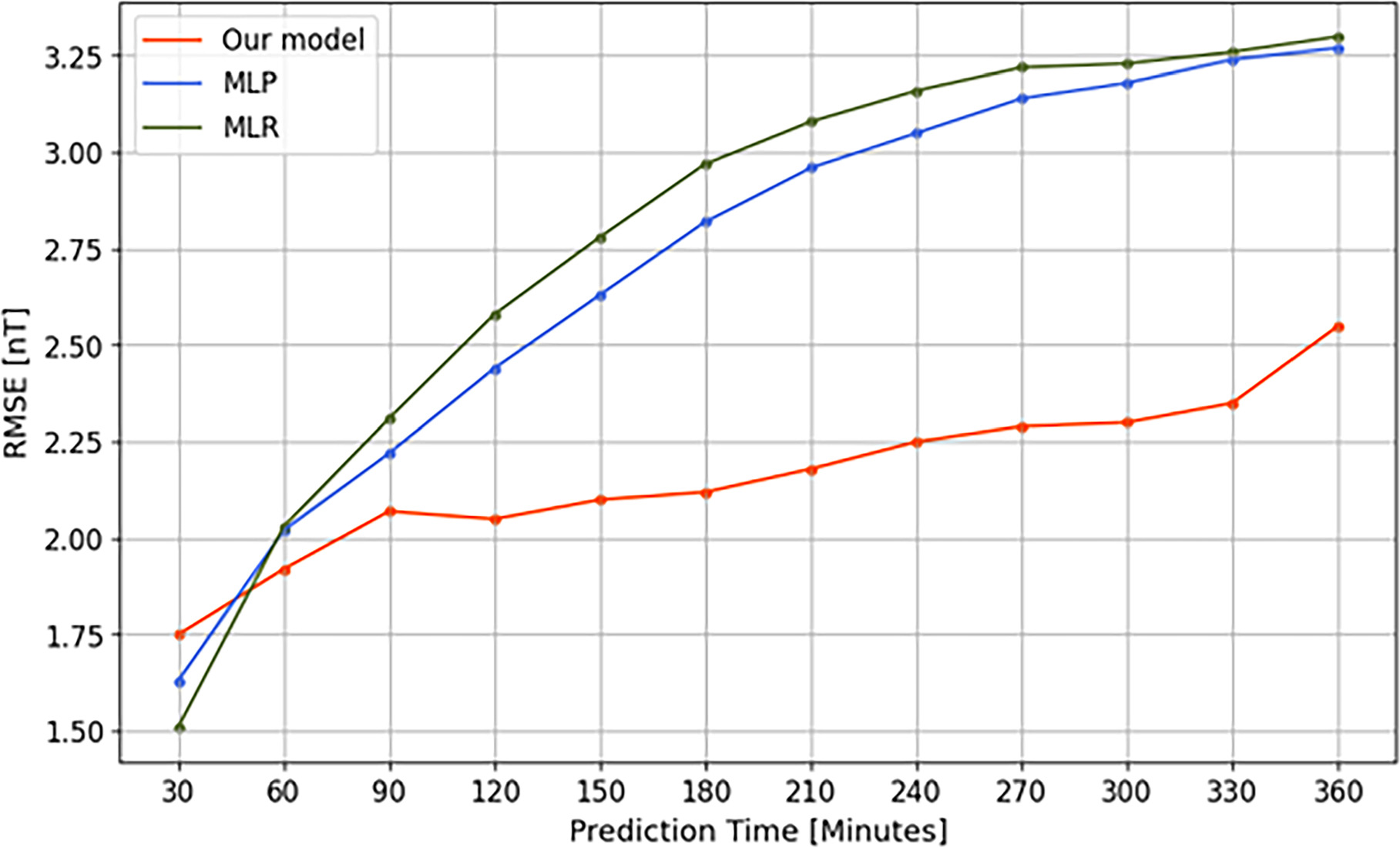
Figure 3. Comparison of the RMSE of the BiLSTM model and two baseline models (MLP and MLR) over the prediction time intervals.
Download figure:
Standard image High-resolution imageWe present the results of our model in three cases: a moderate case (Bz ≈ −10 nT), a strong case (Bz ≈ −25 nT), and an extreme condition (Bz ≈ −50 nT; Figure 4). The red dashed line indicates the prediction time, and the green solid line indicates the target data. The results of the ensemble model are represented by the red solid line, with the shaded area indicating the prediction range. For each plot, only the models whose test sets overlap with the target period are included. The predictions of these overlapping models are averaged to generate the final results shown in Figure 4.
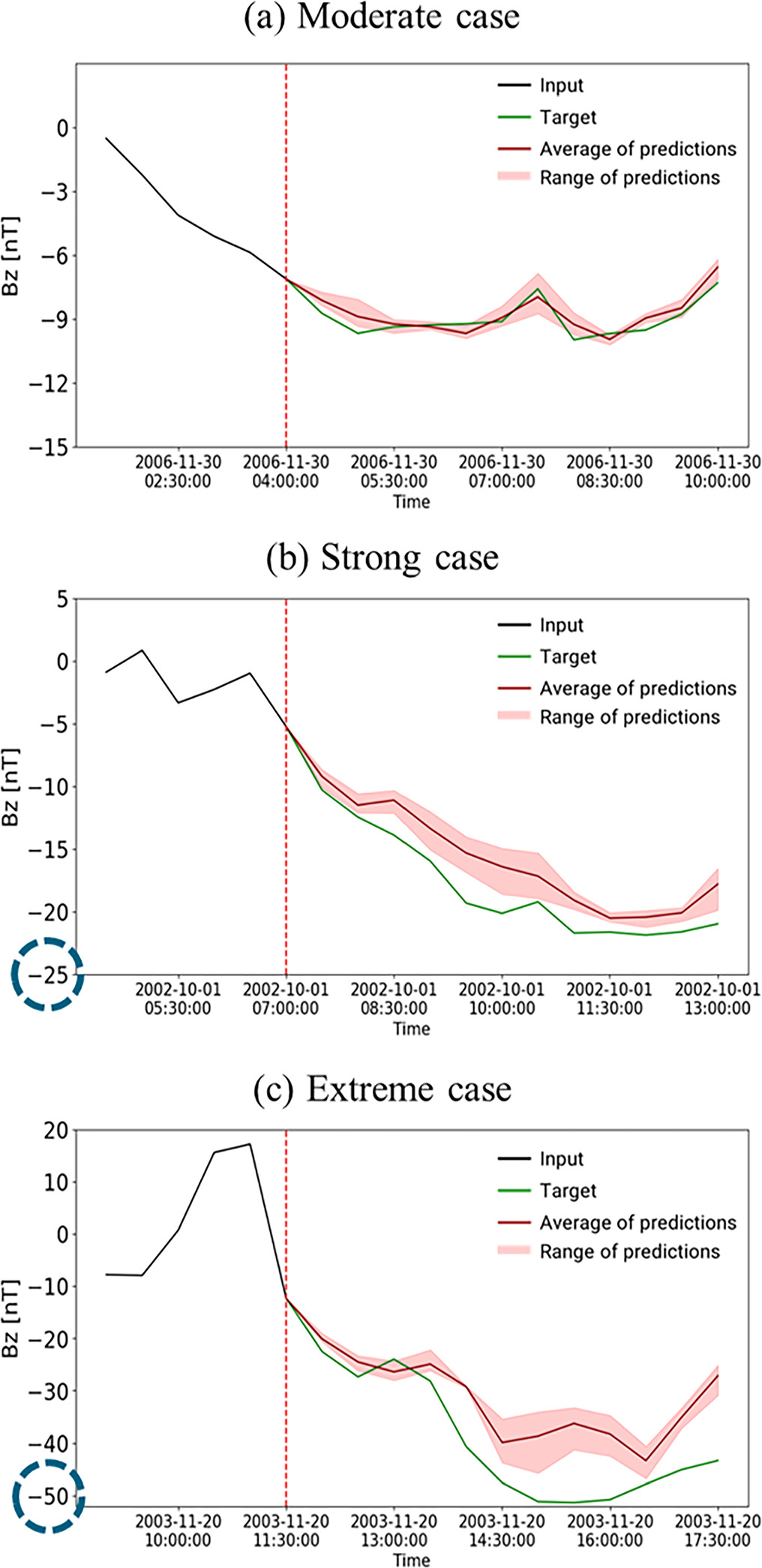
Figure 4. Results of our model predictions across three geomagnetic conditions: (a) moderate case, (b) strong case, and (c) extreme case. The green solid line indicates the target data, and the red solid line shows the average prediction from our model ensemble of 12 individual models. The red shaded area represents the prediction range. The red dashed vertical line marks the prediction time onset.
Download figure:
Standard image High-resolution imageIn the moderate condition, the Bz component remains relatively stable with minor fluctuations. Our model closely tracks the observed Bz values throughout the prediction period. The small deviations in the predictions are well made within acceptable limits, indicating that the model is effective at capturing the slight variations typical of quiet periods. In the strong case, where the Bz component exhibits a more pronounced decline, our model continues to track the target closely, with slightly larger but still well-contained prediction intervals. The extreme condition presents a more challenging variation to predict, characterized by sharp declines and significant fluctuations in the Bz component. Despite the increased complexity, the model demonstrates a strong ability to capture the overall downward trend. However, an error of approximately 20 nT at the peak reflects a limitation of the deep learning model. This is likely due to the rarity of such extreme cases in the training data. Nevertheless, the broader uncertainty range observed here points to the difficulty of predicting highly unstable conditions, though the model performs well in most other periods.
Overall, these results suggest that the model effectively captures information from the input solar wind parameters, including the previous near-Earth information just before, enabling the model to perform well even without direct data from the solar source region. The BiLSTM’s architecture appears particularly well suited to modeling the nonlinear dependencies within the data, contributing to its robust performance across varying space weather conditions.
We evaluate our model using a separate test data set from the years 2023–2024, which is not used during training or validation in any of our models. This data set serves as a truly out-of-sample evaluation to assess the generalization performance of our model. The evaluation results are presented as boxplots in Figure 5. The central line inside each box represents the median, which offers a robust measure of central tendency. The box itself covers the interquartile range (IQR), representing the middle 50% of the data, while the whiskers extend to the minimum and maximum values within 1.5 times the IQR. The size of the box indicates the variability of the predictions: smaller boxes represent more consistent predictions. These boxplots are the results from all 12 independent models, providing a comprehensive view of the model’s performance across the multiple data splits. Our model consistently outperforms the baseline MLP across all prediction times in terms of RMSE, mean absolute error (MAE), and correlation coefficient (CC). While some variability remains, the superior median performance indicates that our model effectively captures complex temporal patterns in the data. These results confirm that our model generalizes well to unseen data.
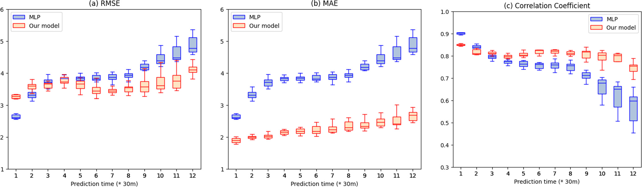
Figure 5. Prediction performance of our model (red) compared to the baseline MLP model (blue) on an independent test data set from 2023 to 2024. (a) RMSE, (b) MAE, and (c) Pearson CC are shown for each prediction time.
Download figure:
Standard image High-resolution imageThe findings of this study have a potential applicability to predicting geomagnetic indices such as Dst, AE, and Kp indices. These indices can be expressed in terms of solar wind speed and southward component of IMF (R. K. Burton et al. 1975; I. Y. Plotnikov & E. Barkova 2007; R. Boroyev & M. Vasiliev 2018). We plan to integrate our model with the solar wind speed prediction model (J. Son et al. 2023) to develop a more comprehensive tool for geomagnetic index forecasting. Such an integrated model could provide earlier and more accurate warnings of geomagnetic storms. Additionally, our model could be applied to global empirical magnetic field models (e.g., N. Tsyganenko 2014) and MHD simulation models (e.g., K. S. Park 2021) of the geomagnetosphere. If the predicted Bz values from our model are used as input data for these models, they would help in predicting the changes in the Earth’s magnetosphere. These applications are left for our future work.
5. Conclusion
In this study, we have developed a deep learning model to predict the strong southward component of the IMF Bz for the next 6 hr, particularly under conditions where Bz values become negative. We have implemented a BiLSTM method using solar wind parameters (V, N, T) and IMF components (Bt, Bx, By, Bz) as input data. Our model’s performance is compared to two baseline models: the MLR and MLP models. The results indicate that our model has a much better performance in view of the RMSE values than those of the baseline models. The RMSE of our model ranges from 1.75 (for 30 minute predictions) to 2.55 nT (for 6 hr predictions). Additionally, the model can track the downward trends of Bz during not only moderate conditions but also strong and extreme conditions, highlighting its potential for short-term predictions.
Despite these promising results, one limitation of our study is that our model is trained and tested only on Bz values below a certain threshold, specifically focusing on more negative trends. As a result, the model has not yet been validated for broader operational use in near-real-time space weather forecasting, where accurate predictions across the full range of Bz values are needed. Nevertheless, it is important to emphasize that this research can be a good starting point in the development of deep learning models for Bz prediction. Our study demonstrates the feasibility of using the deep learning method to predict Bz.
Predicting the Bz component is crucial for space weather forecasting as it plays a key role in driving geomagnetic storms that can affect various systems. By advancing the capability to predict Bz, our research contributes to the broader goal of improving space weather forecasting, thereby enhancing preparedness and minimizing the potential impacts of space weather events.
Acknowledgments
This work was supported by the Korea Astronomy and Space Science Institute under the R&D program (Project No. 2024-1-850-02), supervised by the Ministry of Science and ICT (MSIT), and by the Institute for Information and Communications Technology Promotion (IITP) grant, funded by the Korea government MSIT (No. RS-2023-00234488, Development of solar synoptic magnetograms using deep learning, 15%). It was also supported by the BK21 FOUR program through the National Research Foundation of Korea (NRF) under Ministry of Education (MoE; Kyung Hee University, Human Education Team for the Next Generation of Space Exploration) and by the NRF grant funded by the Korea government (MSIT; RS-2024-00346061), as well as the Basic Science Research Program through the NRF funded by the MoE (RS-2023-00248916). This research is (partially) funded by the BK21 FOUR program of Graduate School, Kyung Hee University (GS-1-JO-NON-20242364). We acknowledge the use of NASA/GSFC’s Space Physics Data Facility’s OMNIWeb service and OMNI data. We also thank the community for their efforts in developing the open-source packages utilized in this work.