Abstract
Dense cores are the final place where turbulence is dissipated. It has been proposed from theoretical arguments that the nonthermal velocity dispersion should be narrower both for molecular ions (compared to neutrals) and for transitions with higher critical densities. To test these hypotheses, we compare the velocity dispersion of  (1–0) (
 = 6 × 10⁴
  ) and
) and  (
( = 2 × 10³
  ), in the dense core Barnard 5. We analyze well-resolved and high signal-to-noise observations of
  (1,1) and (2,2) obtained with combining Robert C. Byrd Green Bank Telescope (GBT) and Very Large Array (VLA) data, and
  (1–0) obtained with GBT Argus, which present a similar morphology. Surprisingly, the nonthermal velocity dispersion of the ion is systematically higher than that of the neutral by 20%. The derived sonic Mach number,
  , has peak values
  and
and  for
for  and
and  , respectively. This observed difference may indicate that the magnetic field even deep within the dense core is still oscillating, as it is in the turbulent region outside the core. The ions should be more strongly dynamically coupled to this oscillating field than the neutrals, thus accounting for their broader line width. If corroborated by further observations, this finding would shed additional light on the transition to quiescence in dense cores.
1. Introduction
Molecular cloud cores, the places where stars form, have been studied using both molecular line transitions of dense gas tracers and dust continuum mapping (Benson & Myers 1989; Kauffmann et al. 2008). One of the most widely used dense gas tracers is  , which traces material with densities of a few 103
 and higher, and thanks to its hyperfine structure, it is useful to determine temperature, density, optical depth, and the kinematic properties of the gas (Myers & Benson 1983; Benson & Myers 1989). By mapping dense cores in
  (1,1), it has been found that they show an almost constant level of nonthermal motions, within a certain coherence zone (Goodman et al. 1998). However, the parental molecular cloud hosting the dense core usually displays highly supersonic line widths (Zuckerman & Evans II 1974; Larson 1981; Brunt & Heyer 2002; Heyer & Brunt 2004; Choudhury et al. 2020). The term “coherent core” is used to describe the dense gas where nonthermal motions are roughly constant, and typically smaller than the thermal motions, independent of scale (see also Caselli et al. 2002a). We have observed the transition from turbulence to quiescence using a single tracer in a few objects at relatively coarse angular resolution (Pineda et al. 2010; Friesen et al. 2017). Additional studies at higher resolution, and employing a variety of tracers, should aid our understanding of dense core structure and formation, and hence the initial conditions for star formation (e.g., Gong & Ostriker 2011; Bailey et al. 2015).
The empirical line-width–size relation, first found by Larson (1981) and refined by Solomon & Rivolo (1989), shows that smaller molecular clouds of higher density are generally more quiescent. Thus, if this relation applies within individual dense cores, we expect that tracers with higher critical density should exhibit narrower line widths (Myers 1983). So, too, should molecular ion tracers, which are dynamically tethered to the dense core’s internal magnetic field. Neutral species, on the other hand, move about more freely, and are imperfectly coupled to the ions via collisions (Mestel et al. 1956). Houde et al. (2000) compared single-dish observations of neutrals and ions for which they see a broader line width for neutrals compared to ions, and derived a relation between the a relation for the line width of the ion and neutral. Their formalism takes into account the collisions between ions and neutrals as particles, under the assumption that ions are forced into gyromagnetic motion about the magnetic field direction, but, it is not a full description of the plasma fluid behavior. Under these assumptions the ions will always display a narrower line width when tracing the same region. Recently, MHD simulations show that in some cases the ions could have more energy than neutrals (Burkhart et al. 2015), however, no clear predictions are made for comparisons with observations inside dense cores (Meyer et al. 2014). In addition, the observations presented in Houde et al. (2000) are single-dish observations toward two active star-forming regions, Orion A and DR21, with an angular resolution between 20″ and 30″, which are insufficient to resolve the outflows and substructures observed at higher angular resolution (e.g., Hacar et al. 2018; Monsch et al. 2018) and might explain the difference in the HCO+ and HCN lines observed.
Surprisingly, Tafalla et al. (2004) found that the levels of turbulence displayed by the  (1–0) line (
 ; Shirley 2015) are higher than those obtained with
  (1,1) (
 ; Shirley 2015) in a few cores observed at coarse angular resolution (40″) insufficient to resolve the core structure. Ostensibly, their finding is at odds with the conventional theoretical picture. Until now, however, no data have been of sufficient angular and spectral resolution to explore the different kinematics of ion and neutral dense gas tracers on well-resolved maps (e.g., Tafalla et al. 2004). Therefore, it has been impossible to accurately measure the velocity differences within the subsonic region or the velocity differences between neutrals and ions in dense cores. Similarly, in recent deep observations of
  and
and  (1–0) in an infrared dark cloud, Sokolov et al. (2019) found that
  displays a nonthermal velocity dispersion 20% lower than
  (1–0). However, those observations lacked sufficient angular resolution to perform a detailed comparison.
Barnard 5 (B5) is an isolated and bright dense core (Langer et al. 1989) in the Perseus molecular cloud (302 ± 21pc; Zucker et al. 2018). Its average density in the region of subsonic turbulence is 
 , and this region includes a single Class I object (the ∼0.5
  B5-IRS1; Fuller et al. 1991) driving a parsec-scale outflow (Langer et al. 1989; Bally et al. 1996; Arce et al. 2010; Zapata et al. 2014). Previous Robert C. Byrd Green Bank Telescope (GBT)
  (1,1) observations (with 30″ angular resolution) of B5 allowed us to detect for the first time the sharp transition between subsonic and supersonic turbulence in a single tracer (Pineda et al. 2010). New
  (1,1) observations of B5 obtained with the Jansky Very Large Array (JVLA; and combined with the GBT single-dish data) showed that the velocity dispersion remains subsonic with little variation even at these high-angular resolutions (6″). These data also revealed the presence of filaments within the quiescent dense core, for which the average radial profile is well fitted by an isothermal cylinder model (Ostriker 1964) and the turbulence is consistently subsonic along them (Pineda et al. 2011). These filaments enclose three high-density bound condensations, which combined with the young Class I object might form a bound quadruple multiple star system (Pineda et al. 2015).
We present new observations of the  (1–0) line with GBT Argus to compare them to those obtained from
  (1,1) to measure possible differences between ions and neutrals throughout the dense core.
2. Observations
2.1. N2H+
We observed the  (1–0) transition line toward B5 using the Argus receiver at the 100 m GBT under project GBT/18B-288 on 2018 October 23 and 25, and on 2018 November 21. Argus is a 16-pixel W-band array receiver, with a 4 × 4 configuration (Sieth et al. 2014), operating between 74 and 116 GHz. We observed the blazar 3C84 (J0319+4130), which is an Atacama Large Millimeter/submillimeter Array (ALMA) calibration source (Bonato et al. 2018, 2019) to obtain the focus and pointing solutions, and to obtain an absolute calibration of the spectra in units of main beam temperature (T
 ). We configured the Versatile GBT Astronomical Spectrometer backend to a rest frequency of 93,173.704 MHz, using mode 4 with 187.5 MHz of bandwidth and 5.7 kHz of spectral resolution. We performed pointing and focus scans every 30–50 minutes, depending on weather conditions. Science scans were obtained in on-the-fly (OTF) mode and calibration scans were done before and after each block of science scans. The system temperatures are ≈118 K for all beams. The observations were carried out using the frequency switching mode, with a frequency shift of 25 MHz (±12.5 MHz shift). We split B5 into two rectangles (2′ × 4′ centered on
  = 03
= 03 47
47 40
4078,
 = +32
= +32 53′43
53′430, and 4′ × 2′ centered on
 = 03
= 03 47
47 37
3735,
 = +32
= +32 50′43
50′436) and scanned both submaps repeatedly in orthogonal scanning directions (i.e., along R.A. and decl.) to reduce the effect of striping and minimize atmospheric instabilities affecting the data quality.
Standard calibration was performed using the GBTIDL package (Marganian et al. 2006) following the procedures and algorithms appropriate for Argus (Frayer et al. 2019). The calibrated data was mapped using the griddata task from the python-based package gbtpipe.
6
At that stage of data calibration we also performed the baseline subtraction, by fitting a polynomial (blorder = 5) to line-free channels before gridding the data. Using a main beam efficiency of 0.46 ± 0.07, we converted from  to
to  . Then we perform a final first-order polynomial baseline removal using the Green Bank Ammonia Survey (GAS) pipeline (Friesen et al. 2017). We smooth the data cube spatially to a final beam size of 8″ and spectrally to a final spectral resolution of 0.049
  using the SpectralCube Python package. The mean rms in the 4′ × 4′ map is 290 mK. The integrated intensity map is calculated over all the hyperfine components and is shown in the left panel of Figure 1. The noise level of the integrated intensity is estimated as 0.4
  using the emission-free region of the map.
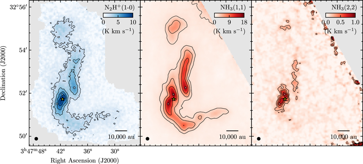
Figure 1. Integrated intensity maps for  (1–0),
  (1,1), and
  (2,2) are shown in left, middle, and right panels, respectively. The contour levels are drawn at [2, 4, 6, 8]
 , [2.4, 4.8, 9.6]
 , and [0.25, 0.4, 0.55, 0.7]
 for the
  ,
,  (1,1), and
  (2,2), respectively. The star and filled circles mark the positions of the Class I object and the condensations identified by Pineda et al. (2015), respectively. The beam and scale bars are shown in the bottom left and right corners, respectively.
Download figure:
Standard image High-resolution image2.2. NH3
We use the  (1,1) and (2,2) data from Karl G. Jansky Very Large Array (VLA) and Green Bank Telescope (GBT) presented in Pineda et al. (2015). The data are a 27-pointing mosaic with the VLA, which is then imaged using multiscale clean and combined with the single-dish data (GBT) using the model image. We finally smooth the data cube to the same angular resolution and regrid the cube to match the
  (1–0) Argus data (8″) using the SpectralCube and reproject Python packages. The typical noise level is 100 mK and 150 mK for the
  (1,1) and (2,2), respectively. The spectral resolution is 0.049
  for both cubes. The integrated intensity maps, calculated over all the hyperfine components, are shown in the middle and right panel of Figure 1. The noise level of the integrated intensity are estimated as 0.3
  and 0.05
  using the emission-free region of the map for the
  (1,1) and
  (2,2) maps, respectively.
3. Results
3.1. Line Fit
We perform the line fit for both species,  and
and  , using the n2hp and cold-ammonia models implemented in pyspeckit (Ginsburg and Mirocha 2011).
The  (1–0) is modeled using the hyperfine structure and relative weights from Pagani et al. (2009) and L. Dore (2011, private communication). The model assumes a Gaussian velocity distribution (with central velocity and velocity dispersion
  and
and  , respectively), equal excitation temperatures (
 ) for all hyperfine components, and total optical depth (
 ). We perform an optically thick fit for the whole cube with all four free parameters, and an optically thin fit with
  as a fixed parameter. We use the results of the optically thick fits, except for pixels where the optical depth has a signal-to-noise ratio less than three (
 ) for which we use the optically thin fit. We discard all velocity determinations if the uncertainty in the
  is larger than 0.02
  .
.
We simultaneously fit the  (1,1) and (2,2) line profiles using the cold-ammonia model (Friesen et al. 2017), which gives a centroid velocity (
 ), velocity dispersion (
 ), kinetic temperature (
 ), excitation temperature (
 ), and total column density of
  (
( , where an ortho-to-para ratio of 1 is assumed). This model assumes that, because of the low kinetic temperatures, only levels (1,1) and (2,2) are populated. The mean value of the kinetic temperature (
 ) in pixels with uncertainty better than 1 K is 9.7 K. For pixels with uncertainties in
  larger than 1 K we rerun the fit, but with a fixed
  of 9.7 K. The kinematic parameters,
  and
and  , are well determined even in cases where the kinetic and excitation temperatures are poorly constrained, thanks to the many hyperfine components. Similarly to
  , we discard all velocity determinations using
  if the uncertainty in the
  is larger than 0.02
  . We consider that the
  and
and  are well determined only when their derived uncertainties are smaller than 1 K, and that the column density is well constrained where
  and
and  are well constrained.
The velocity dispersion derived from both species are further corrected by the channel response

where  is the resulting velocity dispersion from the fit, and
  is the channel width from the observations, 0.049
  for
for  and
and  .
.
Some representative spectra are shown in the Appendix, with the best-fit models. There we show that the models are a good fit, and that there are no strong non-LTE effects on the  (1–0) line which could affect the reliability of the derived kinematical parameters.
3.2. Comparison between Tracers
The centroid velocity maps for both tracers are shown in Figure 2. The same color scale and stretch is used between the left and right panels to allow a direct side-by-side comparison. The centroid velocity maps for both tracers show a similar pattern, and it suggests that both trace similar material. The left panel of Figure 3 shows the comparison of the centroid velocity obtained for both tracers using kernel density estimation (KDE; Virtanen et al. 2020), which agrees within 0.05  . For the KDE determination we use a relative weight for each data point of
  . This comparison shows that there is not a single velocity offset between the different tracers. The right panel of Figure 3 shows the difference in velocity maps between the ions and neutrals. This map shows that neutrals display mostly redder velocities than ions, but that in a few regions the relation is the reverse, although without a clear spatial trend.
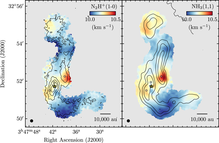
Figure 2. Centroid velocity maps. Left and right panels show the results for  and
and  , respectively. The contours are shown for the
  and
and  (1,1) integrated intensity maps for the left and right panel, respectively, with levels the same as in Figure 1. The star and gray circles mark the positions of the Class I object and the condensations identified by Pineda et al. (2015), respectively. The beam and scale bars are shown in the bottom left and right corners, respectively.
Download figure:
Standard image High-resolution image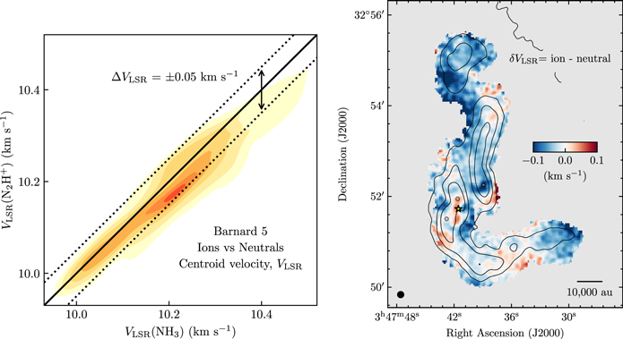
Figure 3. Left: comparison between centroid velocity of  and
and  , estimated using a two-dimensional kernel density estimation (KDE). The one-to-one line is marked by the black solid line, as well as offsets of ± 0.05
  with the dotted lines. Right: spatial map showing the difference between the ion and neutral centroid velocity (
 (
( )−
)− (
( )). Blue hues show that ions present a smaller centroid velocity than neutrals. The contours are shown for the
  (1,1) integrated intensity map, with levels that same as in Figure 1. The star and gray circles mark the positions of the Class I object and the condensations identified by Pineda et al. (2015), respectively. The beam and scale bar are shown in the bottom left and right corners, respectively.
Download figure:
Standard image High-resolution imageThe velocity dispersion map for both tracers are shown in Figure 4. The same color scale and stretch is used between left and right panels to allow a direct side-by-side comparison. The velocity dispersion maps for the two tracers also show a similar pattern, as seen in Figure 4. In this figure, the two distributions of velocity dispersion look quite similar.
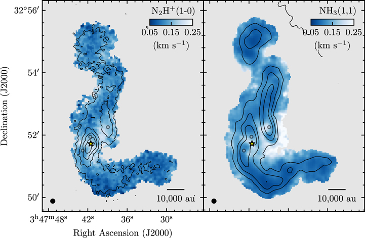
Figure 4. Velocity dispersion maps for  and
and  are shown in the left and right panels, respectively. The contours are shown for the
  (1–0) and
  (1,1) integrated intensity maps for the left and right panel, respectively, with levels the same as in Figure 1. The star and gray circles mark the positions of the Class I object and the condensations identified by Pineda et al. (2015), respectively. The beam and scale bars are shown in the bottom left and right corners, respectively.
Download figure:
Standard image High-resolution imageHowever, a direct comparison of the velocity dispersion distributions for all pixels, see Figure 5, shows that  velocity dispersions are systematically narrower than those derived using
  by
by 
 . We calculate the ratio between the velocity dispersion obtained between
  and
and  (
( ), see Figure 6, which shows that the velocity dispersion of
  is systematically larger throughout the area observed. There is not clear regional or morphological trend, except that the only places where the velocity dispersion of
  is broader than that of
  are close the edge of the map. It is possible that since
  (1,1) can also be excited at densities around 103
 and our observations are deep, then these
  observations are capable of detecting the brighter pixels of the broader
  lines seen during the transition to coherence, previously detected at coarser resolution (Pineda et al. 2010; Friesen et al. 2017; Choudhury et al. 2020).
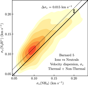
Figure 5. Comparison between the velocity dispersions derived from  (1–0) and
  (1,1), estimated using a two-dimensional KDE. It clearly shows that the
  (higher density tracer and ion) has a systematically broader velocity dispersion than
  (lower density tracer than
  and a neutral). The one-to-one line is marked by the black solid line, while the dotted line marks
  0.015
0.015  .
.
Download figure:
Standard image High-resolution image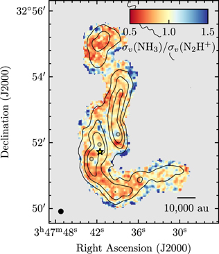
Figure 6. Ratio of the velocity dispersion between  (1,1) and
  (1–0). The prevalence of the red hues shows that
  displays lower velocity dispersion across most of the core than
  . The contours are shown for the
  (1,1) integrated intensity map, with levels the same as in Figure 1. The star and gray circles mark the positions of the Class I object and the condensations identified by Pineda et al. (2015), respectively. The beam and scale bars are shown in the bottom left and right corners, respectively.
Download figure:
Standard image High-resolution image3.3. Nonthermal Velocity Dispersion Comparison
Thanks to the well-constrained kinetic temperature,  , from the
  observations, we estimate the thermal component of the velocity dispersion,
  , to derive a nonthermal velocity dispersion,
  , as
, as

where  is the thermal velocity dispersion of the observed species,

where μ is the molecular weight of the species studied,  is the hydrogen mass, and
  is the Boltzmann’s constant.
The comparison between the different species is shown in Figure 7, which shows that  displays systematically and significantly higher levels of the nonthermal component, about 0.03
  , than
  .
.
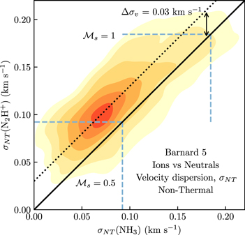
Figure 7. Comparison of the nonthermal velocity dispersions derived from  (1–0) and
  (1,1), estimated using a two-dimensional KDE. It clearly shows that the
  (higher density tracer and ion) has a systematically broader velocity dispersion than
  (lower density tracer than
  and a neutral). The one-to-one line is marked by the black solid line, while the dotted line marks
  0.03
0.03  . The light blue lines mark the sonic Mach number values of 0.5 and 1 for the gas at 9.7 K and a mean molecular weight of 2.37 × mH.
Download figure:
Standard image High-resolution imageWe determine the level of nonthermal velocity dispersion ( ) for both species using the kinetic temperature measured from
  and Equation (2). The sonic Mach number of the turbulence is estimated as

where cs
is the sound speed of the mean particle (using Equation (3) with  ; Kauffmann et al. 2008).
Figure 8 shows the distribution of Mach numbers for the two tracers using KDE. The  distribution, shown in blue, displays a Mach number much smaller (median value of 0.48) than the one in
  (median value of 0.59). This substantial difference in the Mach number is present independently on the actual kinetic temperature used, because already the velocity dispersion comparison shows the same trend, while the thermal component of
  should be larger than that of
  because of the smaller molecular weight.
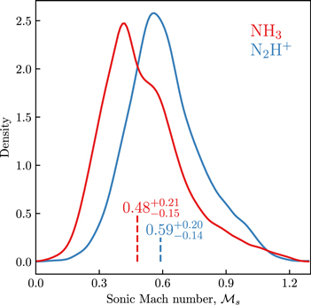
Figure 8. Sonic Mach number distributions for  and
and  , estimated using KDE, are shown in blue and red, respectively. The median values of each sample are marked by the vertical dashed lines. It clearly shows that the
  (higher density tracer and ion) displays a larger sonic Mach number than
  (lower density tracer than
  and a neutral). The sonic Mach numbers are derived using
  as the gas temperature and a mean molecular weight of 2.37 × mH.
Download figure:
Standard image High-resolution imageThe observations analyzed already resolve the substructure found in the coherent region, the filaments, and the fragments. If the difference in the observed velocity dispersions were due to still unresolved substructure with more complex gas dynamics, then this disagreement would be lower in regions away from the higher density filaments. However, the difference is also seen in the surrounding material and lower density regions of the filament. This suggests that the difference is not due to unresolved structures in the region.
4. Discussion
The comparison of both the morphology of the integrated intensity and the similar pattern seen in the centroid velocity (see Figures 1 and 2) suggests that  and
and  trace similar structures and therefore the direct comparison is fair.
4.1. Comparison to Previous Predictions
The critical densities for  (1,1) and
  (1–0) at 10 K are 2 × 10³
 and 6 × 10⁴
 , respectively (see Shirley 2015). If these transitions are tracing material close to these critical densities, and if higher density gas is concentrated in smaller volumes, then
  should trace larger scales than
  . Indeed, our observations of B5 presented in Figure 1 confirm that in B5 the neutrals (
 ) trace scales larger than the ions (
 ; see also Pineda et al. 2010). Finally, simulations of the turbulent cascade (Ballesteros-Paredes et al. 2007) imply that the transition tracing smaller scales (the higher density tracer) do present the smaller Mach number.
Similarly, the presence of static magnetic fields in this star-forming region would give the ions, which are tethered to the field, a smaller velocity dispersion than the neutrals (Li & Houde 2008). For the tracers used in this work the predictions from Houde et al. (2000) and Li & Houde (2008) are opposite to our observations.
4.2. Magnetic Support of Barnard 5
Despite the large mass seen in the coherent core, there is no evidence of large-scale infall motions (Campbell et al. 2016), suggesting that the whole region is not undergoing a dynamical collapse. However, there is not sufficient support against gravity by turbulence, therefore other components might help provide support to this region.
By analyzing more carefully the structure of the filaments, we have estimated an upper limit to the magnitude of the static magnetic field required to support them as  500μG (Schmiedeke et al. 2021) using the relation from Fiege & Pudritz (2000), this magnetic field strength is larger than those estimated in other starless cores (∼200 μG; Liu et al. 2019; Crutcher et al. 2004).
4.3. Penetration by Magnetohydrodynamic Waves
The transition to coherence that demarcates the outer boundary of dense cores is only partially understood, and remains a topic of ongoing investigation. Several recent studies, also observing the  (1,1) line, found this transition to be remarkably sharp, less than 0.04 pc in spatial extent (Pineda et al. 2010; Friesen et al. 2017; Chen et al. 2019; Auddy et al. 2019) In particular, the sudden decrease in the velocity dispersion seen in the neutrals may not apply to the ions.
Ever since the discovery of supersonic motions in the larger cloud medium, it has been proposed that these supersonic line widths indicate the presence of MHD waves (Arons & Max 1975). Of the possible modes, most power is probably contained in Alfvén waves, which are incompressible and therefore less subject to dissipation (Zweibel & Josafatsson 1983). Of course, it is only the charged species that respond directly to the fluctuating magnetic field. Neutrals are coupled via collisions to the ions. In a static, or slowly changing, field, the two species undergo the relative slip that constitutes ambipolar diffusion (Mestel et al. 1956). The same slippage occurs in rapidly fluctuating MHD waves, as was shown in the classic study of Kulsrud & Pearce (1969), see also (Mouschovias et al. 2011) for a more recent overview.
Our confirmation of enhanced line widths for ions with respect to neutrals in the deep interior of B5 suggests a modification to the picture for the transition to coherence. Entering the core from the outside, the steep rise in ambient density leads to a falloff in ion fraction, and therefore in dynamical coupling between ions and neutrals. In particular, the sudden decrease in neutral velocity may not be present in either the ions or the MHD waves impinging on the core.
Both species in our study have subsonic nonthermal velocity dispersions. Thus, the vigorous waves permeating the external medium are damped further inside. This damping is caused by ion–neutral friction. The waves persist into the deep interior, but at reduced amplitude. At the core boundary, where neutral velocities are sharply reduced, the waves fluctuations undergo a more gradual transition. As always, the ions track the wave motion, and thus have higher velocity dispersion. If this picture is correct, it should be possible to corroborate with additional observations of both charged and neutral species.
4.3.1. Wave Amplitude
In the case where ions and neutrals are not perfectly coupled, then we can relate the ion and neutral velocities using Equation (10.19) from Stahler & Palla (2005),

where ω is the wave frequency,  is the frequency with which a given natural atom or molecule is struck by ions,
  is the perturbation on the neutral’s velocity, and
  is the perturbation on the ion’s velocity. Moreover, in this region ω and the wavenumber, k, are related in the long wavelength limit (Pinto et al. 2012) as

which is Equation (10.21) from Stahler & Palla (2005), where Bo
is the unperturbed magnetic field and  is the gas density. Finally, the wave dispersion relation (Equation 10.17 from Stahler & Palla 2005) relates the perturbation in the magnetic field,
  , as
, as

Note that in Equations (5), (6), and (7), ω is complex and can be written as  .
.
We estimate the amplitude of the velocity perturbations as the velocity dispersions,  , derived from the spectral lines
7
and therefore rewrite Equation (5) as
, derived from the spectral lines
7
and therefore rewrite Equation (5) as

where  is the imaginary component, and we define
  .
.
Now, Equation (6) can also be rewritten as
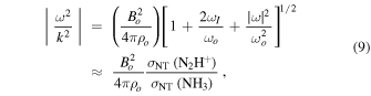
which relates ω and k with observables quantities.
Combining Equations (7), (8), and (9) we obtain

or

which reveals that the magnetic field perturbation is independent on the mean magnetic field strength, but dependent on the density of the gas traced and the geometrical mean of the ions and neutral nonthermal velocity dispersions observed.
The term ni is estimated using the ionization degree,

from Caselli et al. (2002b), which is appropriate for dense cores where there is depletion. The term relating the ion and neutral collisions is approximated by the Langevin term,

for HCO+–H2 collisions (McDaniel & Mason 1973).
For the values obtained inside the coherent core, median, and 1σ spreads of the distributions 
 and
and 
 , we estimate the

which is at least 5% of the magnetic field strength estimated inside the coherent core.
4.3.2. Estimate of Wavelength
Another important parameter to constrain is the wave’s wavelength,

The frequency inside the core,  , can be estimated if we assume that the imaginary component
  is relatively small. Then Equation (8) becomes

and therefore can be used to estimate the wavelength inside the coherent core as

In the case of B5, we obtain a value of  0.64pc, which is larger than the diameter of the coherent core (0.34 pc). However, a direct estimation of the magnetic field strength using dust polarization measurements would substantially improve this estimate of the wavelength. The critical length for wave propagation is obtained from Equation (10.23) of Stahler & Palla (2005) or Equation (79) from Mouschovias et al. (2011),

which we combine with Equation (17) to write

Therefore, the wavelength is sufficient to propagate the wave. In addition, the characteristic damping timescale is given by Equation (80) in Mouschovias et al. (2011),

where the Alfvén velocity is a function of density and magnetic field strength,

Replacing relations 17 and 20 we obtain

which is much smaller than the crossing time of the coherent region

and therefore the waves must be continually injected if they are to persist for a crossing time.
4.4. Future Observations
Since it is unknown how the amplitude of the penetrating wave damps inside the coherent dense core, it is important to take advantage of Equation (11) and observe different pairs of ion and neutral transitions with similar critical densities. This would allow us to derive a damping of the penetrating wave in the subsonic region, which will be crucial to improve our understanding of this newly observed phenomenon.
One promising higher density tracer ion–neutral pair is N2D+ (1–0) and o-NH2D (1 –1
–1 ). These deuterated species are abundant in the densest regions of dense cores (e.g., Caselli et al. 2002b; Crapsi et al. 2007) and they selectively trace higher densities compared to the nondeuterated ones. It is also important that both these transitions have well-known hyperfine structure, which enables for a precise determination of the velocity dispersion. Such comparison will provide a direct determination (or a strong upper limit) of the penetrating Alfvén wave damping. These results would be a new direct observable constraint on the fragmentation process for numerical simulations including magnetic fields.
5. Summary
We present new GBT Argus 8″ angular resolution observations of the Barnard 5 region in the  (1–0) line and compare them with matched beam
  (1,1) and (2,2) VLA and GBT observations. Our results can be summarized as follows.
- 1.Both tracers,
 and , show the presence of two filaments within the subsonic region (coherent core).
 - 2.The centroid velocity maps for and display a similar pattern, with centroid velocities in agreement within 0.05 .
- 3.The velocity dispersion maps show a narrow velocity dispersion throughout the region, but the line displays broader velocity dispersion than by about 0.015 .
- 4.The sonic Mach number for, 0.48, is smaller than for , 0.59, opposite to theoretical predictions of turbulent cascade or ambipolar diffusion for a static magnetic field.
- 5.The difference in sonic Mach number does not appear to be related to unresolved substructures, and it is fairly constant throughout the coherent core.
- 6.The observed difference between ions and neutrals is naturally explained by a penetrating Alfvén wave inside the coherent region, which affects the ions more than the neutrals. We estimate that the associated perturbation in the magnetic field is 27 μG, which is at least 5% of the previously estimated upper limit on the field in the region (500 μG; Schmiedeke et al. 2021).
- 7.The wave’s wavelength is three times the critical wavelength, and it can propagate in the medium. Also, the damping timescale is times shorter than the sound wave crossing time of the coherent region, and therefore waves must be continually injected.


J.E.P., P.C., and A.S. acknowledge the support by the Max Planck Society. This material is based upon work supported by the Green Bank Observatory, which is a major facility funded by the National Science Foundation operated by Associated Universities, Inc. This research made use of APLpy, an open-source plotting package for Python. This research made use of Astropy, 8 a community-developed core Python package for Astronomy. J.E.P. thanks Stella Offner and Ralf Klessen for valuable discussions. We thank Paul Goldsmith, Stella Offner, Daniele Galli, Marco Padovani, Blakesley Burkhart, Shantanu Basu, and the anonymous referee for insightful comments that improved this paper.
Facilities: GBT - Green Bank Telescope, VLA. -
Software: Aplpy (Robitaille & Bressert 2012; Robitaille 2019), Astropy (Astropy Collaboration et al. 2013, 2018), Matplotlib (Hunter 2007), SciPy (Virtanen et al. 2020), pyspeckit (Ginsburg and Mirocha 2011), spectral-cube (Ginsburg et al. 2019).
Appendix: Sample Spectra and Best-fit Model
We show the  (1–0) and
  (1,1) spectra toward a sample of representative regions in the map. The left panel of Figure 9 shows the
  (1,1) integrated intensity map (as in Figure 1) with blue circles marking the positions for the shown spectra. The positions selected include: (A) peak of B5-Cond1, (B) high column density in the narrow filament, (C) isolated dense core at the north, (D) lower column density in the filament, and (E) low column density outside the filaments but inside the coherent zone. The
  and
and  spectra toward position A are shown in Figure 9, positions B and C are shown in Figure 10, and positions D and E are shown in Figure 11. The data in these figures are shown in black, while the best-fit models are shown in red, and the residuals (model data) are shown offset and in gray. In general, all these figures show that the best models provide a good fit to the data.
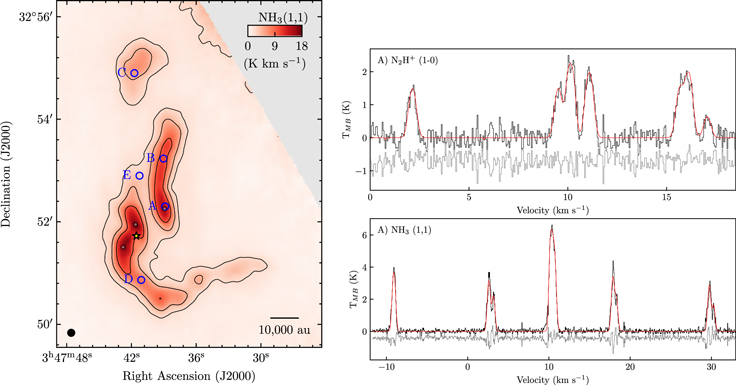
Figure 9. Left: integrated intensity map of  (1,1), as in Figure 1. The blue circles show the positions of the sample spectra. Right: spectra obtained toward position A are shown. Top and bottom panels show the
  (1–0) and
  (1,1), respectively. The data are shown in black, the best-fit model in red, and residual (model data) is shown in gray (but offset for clarity).
Download figure:
Standard image High-resolution image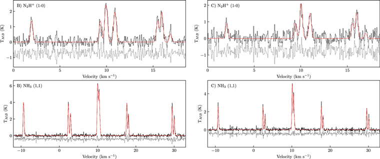
Figure 10. Spectra obtained toward positions B and C are shown in the left and right panels, respectively. The top and bottom panels are the same as in Figure 9.
Download figure:
Standard image High-resolution image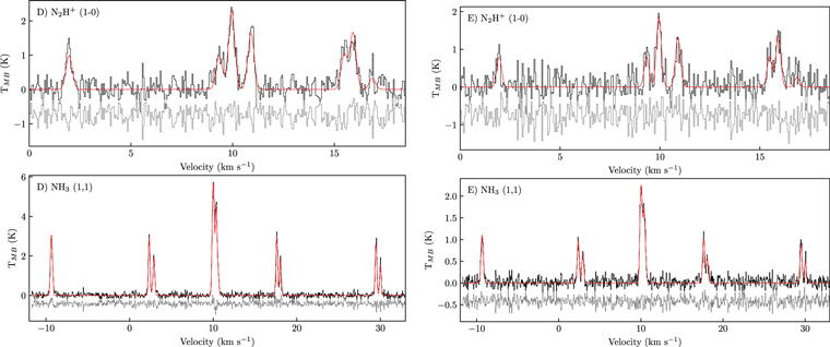
Figure 11. Spectra obtained toward positions D and E are shown in the left and right panels, respectively. The top and bottom panels are the same as in Figure 9.
Download figure:
Standard image High-resolution imageFootnotes
- 6
- 7
This relates the dispersion and amplitude of a sinusoidal wave.
- 8