Abstract
We study the spectral diversity of Type Ia supernovae (SNe Ia) at maximum light using high signal-to-noise spectrophotometry of 173 SNe Ia from the Nearby Supernova Factory. We decompose the diversity of these spectra into different extrinsic and intrinsic components, and we construct a nonlinear parameterization of the intrinsic diversity of SNe Ia that preserves pairings of “twin” SNe Ia. We call this parameterization the “Twins Embedding.” Our methodology naturally handles highly nonlinear variability in spectra, such as changes in the photosphere expansion velocity, and uses the full spectrum rather than being limited to specific spectral line strengths, ratios, or velocities. We find that the time evolution of SNe Ia near maximum light is remarkably similar, with 84.6% of the variance in common to all SNe Ia. After correcting for brightness and color, the intrinsic variability of SNe Ia is mostly restricted to specific spectral lines, and we find intrinsic dispersions as low as ∼0.02 mag between 6600 and 7200 Å. With a nonlinear three-dimensional model plus one dimension for color, we can explain 89.2% of the intrinsic diversity in our sample of SNe Ia, which includes several different kinds of “peculiar” SNe Ia. A linear model requires seven dimensions to explain a comparable fraction of the intrinsic diversity. We show how a wide range of previously established indicators of diversity in SNe Ia can be recovered from the Twins Embedding. In a companion article, we discuss how these results can be applied to the standardization of SNe Ia for cosmology.
1. Introduction
Type Ia supernovae (SNe Ia) are a relatively homogeneous class of luminous astronomical transients. As a result of their homogeneity, SNe Ia can be used as “standard candles” to infer the relative distances to them. The use of SNe Ia as standard candles led to the initial discovery of the accelerating expansion of the universe (Riess et al. 1998; Perlmutter et al. 1999), and as part of a local distance ladder, SNe Ia provide some of the best constraints on the Hubble constant (H0; Riess et al. 2016, 2019). SNe Ia are not all identical, and understanding the diversity of SNe Ia is crucial for our ability to use them for cosmology. It is not currently possible to model the physics of explosions of SNe Ia from first principles to the accuracy required for cosmology. Instead, cosmological analyses of SNe Ia rely on empirical models and corrections to parameterize the observed light curves and infer the relative distances to individual SNe Ia.
1.1. The Diversity of SNe Ia
Initial methods to standardize the luminosities of SNe Ia involved correcting the observed peak brightnesses of SNe Ia for correlations with the widths of their light curves (Phillips 1993) and their B − V colors at maximum light (Riess et al. 1996; Tripp 1998). Current cosmological analyses fit the light curves of each SN Ia using an empirical model of the time-evolving spectral energy distribution (SED). The most commonly used such model, SALT2 (Guy et al. 2007, 2010; Betoule et al. 2014), has one component c for the color and one component x1 for the intrinsic diversity that effectively captures the width of the light curve. With the SALT2 model, the luminosities of SNe Ia can be estimated with an accuracy of ∼0.15 mag, and the distance to an individual SN Ia can be inferred with an accuracy of ∼8%.
Light-curve width and color have been shown to not be sufficient to capture all of the diversity of SNe Ia. Most notably, the inferred SALT2 luminosities of SNe Ia show differences of ∼0.1 mag when comparing SNe Ia in host galaxies with different masses, metallicities, colors, or star formation rates (Kelly et al. 2010; Sullivan et al. 2010; D’Andrea et al. 2011; Gupta et al. 2011; Childress et al. 2013; Hayden et al. 2013; Rigault et al. 2013, 2015, 2020; Roman et al. 2018). These observed differences with host-galaxy properties imply that there is additional unmodeled variability of SNe Ia.
One major open question is to determine the dimensionality of SNe Ia, or how many different modes of variability there are. This is a somewhat ill-posed question: SNe Ia are the result of highly complex explosions and undoubtedly require a parameter space with a very large number of dimensions to fully capture all of their intrinsic diversity. Certain physical components presumably have a very large effect on the observed spectral time series of SNe Ia, such as the composition of the white dwarf (Timmes et al. 2003), total ejecta mass (Scalzo et al. 2014), amount of 56Ni produced (Arnett 1982), photosphere ejecta velocity (Foley et al. 2011), or asymmetry of the explosion (Maeda et al. 2011). Other physical components may only be observable with highly specialized observations with limited effect on the full spectral time series, perhaps including blueshifted Na i D lines (Phillips et al. 2013), the presence of unburned carbon (Thomas et al. 2011), or polarization (Wang & Wheeler 2008). For the purposes of cosmology, it is important to consider that we are only required to model components that have a non-negligible effect on the estimated intrinsic luminosity of SNe Ia at maximum light. Furthermore, all of these observational signatures of diversity are likely correlated and caused by a smaller number of underlying parameters of the explosion.
There have been many efforts to empirically identify modes of variability of SNe Ia other than light-curve width and color. Nugent et al. (1995) showed that ratios of the equivalent widths of the Si ii 5972 Å and Si ii 6355 Å lines map out a spectral sequence of SNe Ia. Branch et al. (2006) used these two lines to separate the spectra of SNe Ia into four subgroups and showed that at least two dimensions are required to parameterize the intrinsic diversity of SNe Ia. Wang et al. (2009) and Foley & Kasen (2011) showed that there is diversity in the velocity of the Si ii 6355 Å feature that is uncorrelated with the width of the light curve and that affects standardization. Further studies have collected thousands of spectra of SNe Ia and have confirmed that the intrinsic diversity of SNe Ia is multidimensional (Blondin et al. 2012; Silverman et al. 2012; Folatelli et al. 2013).
The Nearby Supernova Factory (SNfactory; Aldering et al. 2002) has collected spectrophotometric time series of hundreds of SNe Ia that have enabled a wide range of new analyses of the diversity of SNe Ia. Using this data set, Nordin et al. (2018) showed that there are at least two components of the intrinsic diversity of SNe Ia in the U band that affect standardization. Léget et al. (2020) showed that the diversity of 13 different spectral features can be explained with an underlying three-dimensional parameter space that they call SUGAR. Saunders et al. (2018) developed the SNEMO model using the full spectral time series from SNfactory directly and found that 15 linear components are required to parameterize the diversity of this data set.
The intrinsic diversity of SNe Ia is complicated to parameterize because a typical variation, such as a change in the expansion velocity of the photosphere, leads to highly nonlinear effects in the observed spectra and photometry. Models such as SALT2, SUGAR, or SNEMO are linear, meaning that they attempt to describe the time-evolving SED of an SN Ia at each wavelength and time as the sum of a set of linear components. Fitting a linear model to nonlinear phenomena will result in a model with many more (redundant) components than a similar nonlinear model. Sasdelli et al. (2016) used deep learning to model the spectra of SNe Ia and showed that a nonlinear four-dimensional parameter space can capture the intrinsic diversity of SNe Ia as well as a 15 component linear model. However, their analysis used the derivative of the spectrum rather than the spectrum directly, which removes information such as the brightness and color that are necessary for standardization. Note that the linearity of a model is distinct from the linearity of standardization using the parameters of that model. For example, Rubin et al. (2015) implement nonlinear standardization in terms of SALT2 parameters, but they are still restricted to using the linear SALT2 model that cannot capture nonlinear spectral variation.
1.2. Supernova Twins
Using observations from SNfactory, Fakhouri et al. (2015, hereafter F15) introduced an alternative method of standardizing SNe Ia. When an underlying physical parameter of the explosion is varied, we would expect to see a relatively smooth sequence in the spectra of SNe Ia. The authors developed a method of estimating the “spectral distance” between any pair of SNe Ia and call pairs with low spectral distances “twins.” Standardization can then be done by inferring the luminosity of a new SN Ia directly from its set of twins. As long as one has a large enough reference sample to span the full range of diversity of SNe Ia, one can find SNe Ia with similar spectra to any new SN Ia. The exact functional form of how the spectrum is affected by changes in some underlying physical parameter of the explosion is irrelevant because the twins method only does local comparisons. The twins method does not provide a parameterization of SNe Ia. Rubin (2020) showed that the statistics of the twins pairings from F15 are consistent with the intrinsic variability of SNe Ia being described by an underlying three to five-dimensional parameter space, although they did not explicitly construct this parameter space.
1.3. Overview
In this work, we extend the twins methodology of Fakhouri et al. (2015) to develop a nonlinear parameterization of the spectral diversity of SNe Ia. Assuming that we have a sample of observed SNe Ia that continuously spans the full range of intrinsic diversity of SNe Ia, we can recover the underlying parameterization by identifying sequences of observed spectra where each spectrum in the sequence has a small spectral distance to its neighbors. We call this parameterization the “Twins Embedding.”
For this analysis, we use a large data set of high signal-to-noise spectra of SNe Ia from SNfactory that is described in Section 2. We perform a sequential analysis to decompose the variability of SNe Ia. First, we model the differential time evolution of the spectra of SNe Ia near maximum light in Section 3, and we estimate the spectra of all of our SNe Ia at maximum light. In Section 4, we introduce a second procedure that we call “Reading Between the Lines” (hereafter RBTL) to estimate the contributions to the spectra from distance uncertainties and dust extinction and produce dereddened spectra of SNe Ia that nominally have only intrinsic variability remaining. Finally, we perform a nonlinear decomposition of the remaining variability of these dereddened spectra in Section 5, and we produce a parameterization of the intrinsic diversity of SNe Ia that we call the “Twins Embedding.” In Section 6, we explore the properties of the Twins Embedding and show how it can be used to recover a wide range of previously studied indicators of intrinsic diversity of SNe Ia. In a companion article (Boone et al. 2021, hereafter Paper II), we show how the Twins Embedding can be used to improve the standardization of SNe Ia.
2. Data Set
For this analysis, we make use of the spectrophotometric time series of SNe Ia obtained by the SNfactory. These spectrophotometric time series were collected using the Super Nova Integral Field Spectrograph (SNIFS; Lantz et al. 2004). The SNIFS spectroscopic channels consist of two lenslet integral field spectrographs (IFS; Bacon et al. 1995, 2001), which split a fully filled 64 × 6
4 field of view into a grid of 15 × 15 spatial elements. The two channels cover the 3200–5200 Å and 5100–10000 Å wavelength ranges simultaneously. A photometric channel simultaneously images the field around the IFS to monitor atmospheric transmission. The SNIFS instrument is continuously mounted on the south bent Cassegrain port of the University of Hawaii 2.2 m telescope on Maunakea.
The spectra from SNIFS were reduced using the SNfactory data reduction pipeline (Bacon et al. 2001; Aldering et al. 2006; Scalzo et al. 2010). The flux-calibration procedure for this pipeline is described in Buton et al. (2013), and the host-galaxy subtraction procedure is presented in Bongard et al. (2011). The spectra were corrected for Milky Way dust using the dust map from Schlegel et al. (1998) with an extinction–color relation from Cardelli et al. (1989).
We fit the light curve of each of the SNe Ia in our sample using the SALT2 light-curve fitter (Betoule et al. 2014) version 2.4 that is currently used for most cosmological analyses with SNe Ia (e.g., Scolnic et al. 2018). To perform these fits, we synthesize photometry from the spectrophotometry in the SNfactory BSNf, VSNf, and RSNf bands, defined as top-hat filters with transmission for wavelengths between 4102–5100, 5200–6289, and 6289–7607 Å respectively. For this analysis, we focus specifically on spectra from the SNfactory data set near maximum light because F15 showed that twin SNe Ia can be identified and standardized just as effectively with a spectrum at maximum light as with a full spectral time series. We use the SALT2 fits to determine the time of maximum light for each SN Ia. To ensure that we have a reasonable determination of these parameters, we require that each SN Ia have at least five spectra and that the SALT2 day of maximum parameter uncertainty is less than one rest-frame day. We then retain all of the spectra within five rest-frame days of maximum light for our analysis.
We preprocess all of our spectra of SNe Ia by shifting the wavelengths of the spectra to the SN Ia’s rest frame, and we adjust their brightnesses so that they appear to be at a common redshift of 0.05. We then rebin the spectra with a common binning of 1000 km s−1 between 3300 and 8600 Å. This results in a total of 288 wavelength bins and is the same binning used in F15 and Saunders et al. (2018). Our analysis is designed to be insensitive to the distances to SNe Ia, so the choice of cosmological parameters is irrelevant.
Although most of the near-maximum spectra are suitable for this study, we find that low signal-to-noise (S/N) spectra from the SNIFS instrument can have relatively large systematic fractional systematic uncertainties at the bluer ends of the spectra. These uncertainties appear to be primarily due to poor fits of the model in the extraction from the CCD, which introduces a correlated offset that gets larger toward bluer wavelengths. We find that these offsets are uncorrelated for repeated observations of the same target. In this analysis, we are interested in understanding the intrinsic spectral diversity of SNe Ia. If present, instrumental sources of spectral diversity would be recovered in such an analysis and potentially confused with intrinsic spectral diversity. To avoid this issue, we require that the total statistical S/N of all of the spectra used in this analysis be larger than 100 when integrated over the bluest 500 Å of the spectrum. We examined the effect of redshift, airmass, seeing, sky background level, properties of standard stars used for calibration on a given night, photometricity of the night, moon location, detector temperatures, time that the detector was on, and many other variables on the observed spectra. For the latest SNfactory spectral reductions, we do not notice any significant relationships between the observed spectra and these properties beyond S/N. One potential issue is that the requirement on S/N in the bluest 500 Å of the spectrum could bias our analysis toward a specific subtype of SN Ia. However, the variation in S/N simply due to the observed brightnesses of SNe Ia at the wide range of different redshifts and sky brightnesses considered is much larger than the intrinsic variation in brightness in this band, and we do not see evidence of significant selection biases when looking at, e.g., SALT2 parameters.
Note that we include SNe Ia in this analysis irrespective of whether they have been labeled as “peculiar.” A summary of the attrition for each of these steps is shown in Table 1. A total of 203 SNe Ia pass all of the previously described selection requirements with a total of 598 spectra within five days of maximum light passing the S/N requirements. This data set is much larger than the sample of 55 SNe Ia used in the original Twins analysis of F15.
Table 1. Summary of Sample Selection Requirements
| Selection Requirement | Number of SNe Ia |
|---|---|
| Passing Requirement | |
| General selection requirements | |
| Initial sample (SNe Ia with at least five SNfactory spectra) | 280 |
| SALT2 date of maximum light uncertainty < 1 day | 272 |
| At least one spectrum within 5 days of maximum light | 250 |
| At least one spectrum with S/N 3300–3800 Å > 100 | 203 |
| Manifold learning selection requirements | |
| (Section 5.2) | |
| Spectrum at maximum uncertainty < 10% of intrinsic variance | 173 |
Note. The general selection requirements, listed in the first section of the table, are applied to all of our analyses. For the manifold learning analyses in Section 5, an additional selection requirement is imposed on the quality of the estimated spectra at maximum light.
Download table as: ASCIITypeset image
3. Estimating the Spectra of SNe Ia at Maximum Light—The Differential Time Evolution Model
Even though we have only included SNe Ia with spectra within five days of maximum light for this analysis, if we were to compare spectra of different SNe Ia to each other directly, their phases could differ by as much as 10 days. The authors of F15 used Gaussian Process (GP) regression to generate models of the spectral time series for each SN Ia, which can then be evaluated at arbitrary phases. This method is very effective when the time series is well sampled, but each SN Ia is fit completely independently of all other SNe Ia, so the GP predictions typically have large uncertainties when estimating the spectra of poorly sampled time series. As a result, the analysis of F15 had very strict requirements on the sampling of the SN Ia light curves near maximum light and was only able to use a limited subset of the SNe Ia in the SNfactory data set at that time.
Instead, in this work, we build a new method of estimating the spectra of SNe Ia at maximum light that simultaneously models the differential time evolution of all SNe Ia in a sample. To build our differential time evolution model, we assume that the time evolution of the flux of SNe Ia near maximum light can be written as a quadratic polynomial in magnitude for each wavelength:

where mi (p; λk ) is the spectrum of SN Ia i in magnitudes at phase p and in the wavelength bin λk . c1(λk ) and c2(λk ) are arbitrary functions of wavelength that are the same for all SNe Ia and that represent the time evolution of SNe Ia near maximum light. Note that we are modeling the differential time evolution relative to maximum light rather than the spectra directly. Any constant multiplicative extrinsic effects such as dust reddening or uncertainties in the distance estimate have no effect on such a differential model.
For a given SN Ia, we label the observed flux of spectrum s as fobs.,s. For spectra observed with SNIFS, we find that along with typical uncorrelated measurement uncertainties σmeas.,s(p, λk
), the individual spectra have gray dispersions mgray,s in brightness with σgray ∼ 0.02 mag independent of wavelength after calibration (Buton et al. 2013). Furthermore, our simple model will not be able to capture all of the diversity in the spectral evolution of SNe Ia. To account for this, we add a term to capture the residual uncertainty of the differential time evolution model as a function of phase. We model this uncertainty as a fraction of the observed flux using a broken linear function (p; λk
) that is fixed to zero at our reference point of maximum light with nodes at −5, −2.5, 2.5, and 5 days for each wavelength bin. For computational reasons, we implement this uncertainty as a fraction of the observed flux, but for consistency with previous literature, we interpret it in the following text as the corresponding difference in magnitudes. Our full model of the observed spectra and the uncertainty on them is then


We implement this model using the Stan modeling language (Carpenter et al. 2017) and simultaneously fit it to our full sample of 598 spectra within five days of maximum light for 203 different SNfactory SNe Ia. For each SN Ia, we fit for a single spectrum at maximum light mi
(0; λk
) that combines the information from all of the different spectra of that SN Ia taken within 5 days of maximum light. With our spectra binned in 288 wavelength bins as described in Section 2, this model has a total of 288 × 203 parameters representing the spectra at maximum light, 288 × 2 parameters for the c1(λk
) and c2(λk
) functions that represent the time evolution of spectra, 288 × 4 parameters for the broken linear function that we use to represent the model uncertainty (p; λk
), 598 parameters for the gray offsets mgray,s of each spectrum, and finally, one parameter for the gray offset dispersion
 .
.
We use Stan to optimize the parameters of this model to obtain the maximum a posteriori probability (MAP) estimate of the model parameters (Carpenter et al. 2017), including the predicted spectrum at the time of maximum light of each SN Ia. We propagate the various sources of uncertainty to obtain an estimate of the uncertainty on the spectrum at the maximum light of each SN Ia. The recovered model parameters are shown in Table 2.
Table 2. Global Parameters of the Differential Time Evolution and Reading between the Lines (RBTL) Models
| Wavelength | Differential Time Evolution Model | RBTL Intrinsic | |||||
|---|---|---|---|---|---|---|---|
| Phase Evolution | Phase Node Uncertainties | Dispersion | |||||
| λk | c1(λk ) | c2(λk ) |
|
|
|
| η(λk ) |
| (Å) | (mag) | (mag) | (mag) | (mag) | (mag) | (mag) | (mag) |
| 3463 | 0.102 | 0.01134 | 0.061 | 0.024 | 0.062 | 0.083 | 0.160 |
| 3801 | 0.049 | 0.00577 | 0.069 | 0.023 | 0.035 | 0.095 | 0.246 |
| 4171 | −0.001 | 0.00944 | 0.035 | 0.011 | 0.059 | 0.120 | 0.072 |
| 4579 | −0.004 | 0.00695 | 0.037 | 0.009 | 0.027 | 0.061 | 0.066 |
| 5026 | 0.014 | 0.00683 | 0.047 | 0.024 | 0.041 | 0.052 | 0.049 |
| 5516 | −0.003 | 0.00601 | 0.055 | 0.008 | 0.044 | 0.056 | 0.089 |
| 6055 | −0.024 | 0.00686 | 0.092 | 0.042 | 0.033 | 0.084 | 0.252 |
| 6645 | −0.011 | 0.00337 | 0.062 | 0.026 | 0.007 | 0.017 | 0.019 |
| 7294 | 0.020 | −0.00046 | 0.075 | 0.046 | 0.022 | 0.039 | 0.047 |
| 8006 | 0.003 | 0.00584 | 0.098 | 0.054 | 0.022 | 0.069 | 0.191 |
| ⋯ | |||||||
Note. A representative selection of 10 lines of this table are shown here. The full table is available in machine-readable version.
Only a portion of this table is shown here to demonstrate its form and content. A machine-readable version of the full table is available.
Download table as: DataTypeset image
This model effectively uses the SNe Ia that have observations at multiple phases to constrain the c1(λk
), c2(λk
), and (p; λk
) parameters that describe the differential time evolution of the spectra of SNe Ia near maximum light. If multiple spectra are available for a given SN Ia, then they will all be used to estimate the spectrum at maximum light. If only a single spectrum is available for a given SN Ia, then the spectrum will not provide any constraints on the differential model parameters, but it can still be used to estimate the spectrum of the SN Ia at maximum light. Examples of this procedure are shown in Figure 1 for SNF 20060621–015 with three observed spectra and SNF 20070712–000 with a single observed spectrum 4.77 days after maximum light.
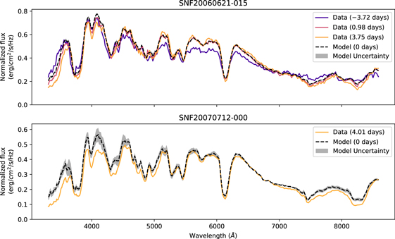
Figure 1. Top: estimated spectrum of SNF 20060621–015 at maximum light. SNF 20060621–015 has three different spectra passing the selection criteria, shown in different colors. The information from all three of these spectra is used to predict the spectrum at maximum light, shown with a dashed black line. A shaded gray contour around this dashed black line shows the uncertainty on the estimate of the spectrum at maximum light. Bottom: estimated spectrum of SNF 20070712–000 at maximum light. SNF 20070712–000 has only a single spectrum passing our selection criteria, but we can still estimate the spectrum at maximum light using the differential time evolution model.
Download figure:
Standard image High-resolution imageThe recovered differential time evolution model described in Equation (1) is shown in Figure 2. Note that we aligned all of our SNe Ia to the SALT2-determined time of maximum light, which is the time of maximum light in the B band, a filter that roughly corresponds to the integrated flux between 4000 and 5000 Å. As expected, our model predicts that the SN Ia gets fainter in either direction relative to maximum light in this wavelength band. We find that the time of maximum light is consistent from roughly 3900–6800 Å. However, for wavelengths bluer than 3900 Å or redder than 6800 Å, we find that the time of maximum light of the light curve occurs significantly earlier. For wavelengths between 3300 and 3500 Å, we find that the light curve declines by up to 0.2 mag day−1, with this decline becoming increasingly rapid at later phases. Similarly, in the redder bands, we find that the light curve declines by up to 0.1 mag day−1 in two regions of the spectrum, corresponding to the O i absorption triplet and the Ca ii IR triplet. If these effects were not taken into account, then the spectrum of an SN Ia observed 5 days after maximum light would have systematic differences of up to 0.8 mag from the true spectrum at maximum light.
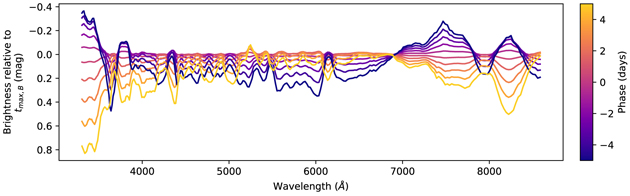
Figure 2. Model of the differential time evolution of SNe Ia near maximum light. The modeled differences are shown in different colors for phases within five days of maximum light with a spacing of one day. The color bar indicates which phase corresponds to which line on this plot.
Download figure:
Standard image High-resolution imageWe show the uncertainty of the differential time evolution model as a function of phase in Figure 3. We find that our model is able to estimate the spectra of SNe Ia for phases within 2.5 days of maximum light with an uncertainty of less than 0.05 mag at almost all wavelengths. For spectra 5 days away from maximum light, the model uncertainties are around 0.05 mag at most wavelengths, but the model is unable to accurately model the time evolution of the Ca ii H&K feature around 3900 Å. Five days before maximum light, the uncertainty of the time evolution of this feature is more than 0.35 mag for the worst wavelengths, indicating that there is significant additional variability in the time evolution at these wavelengths that is not captured by a model that only takes into account the phase of the spectrum. To test the accuracy of the uncertainty model, we examined pairs of spectra where one is very close to maximum light and used the differential time evolution model to estimate the flux of a second spectrum at a different phase. We verified that the observed residuals are consistent with the uncertainty model.
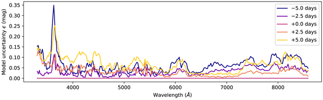
Figure 3. Differential time evolution model uncertainties (p; λk
) as a function of wavelength for different phases. Note that the model uncertainty at maximum light is zero by definition.
Download figure:
Standard image High-resolution imageThis differential time evolution model does not take the intrinsic variability of SNe Ia into account and only corrects for the behavior common to all SNe Ia. Averaged over all wavelengths, we find that 84.6% of the variance in the evolution of spectra near maximum light is common to all SNe Ia and thus captured by our differential time evolution model. As a test, we ran a variant of our model from Equation (1) that includes a correction for SALT2 x1 as a proxy for intrinsic variability with the following functional form:
We find that this model explains 86.9% of the variance in the evolution of spectra near maximum light, which is only a slight improvement over our fiducial model. This implies that the majority of the remaining variability is unrelated to the SALT2 x1 parameter. Furthermore, we find that there are no significant differences in the results of the rest of our analyses when we include or exclude SALT2 x1 from the differential time evolution model. Note that not including SALT2 x1 or any other parameterization of the intrinsic diversity of SNe Ia in the differential time evolution model slightly increases the model uncertainties, but we propagate those uncertainties to further analyses so they should not affect our results.
4. Reading between the Lines
After applying the differential time evolution model, we have estimates of the spectra at maximum light for all of the 203 SNe Ia in our analysis, along with uncertainties on those estimates. Our objective is to decompose the diversity of those spectra. There are two known extrinsic contributions to the diversity of the remaining spectra that are unrelated to the intrinsic diversity of SNe Ia. First, in Section 2, we used the observed redshifts of the host galaxies of SNe Ia to estimate the relative distances to them and shift them to a common redshift. The observed host-galaxy redshift is not a perfect measurement of the cosmological distance to an SN Ia, and it also contains contributions from peculiar velocities of the host galaxies (Davis et al. 2011) among other factors. These uncertainties in the relative distances to SNe Ia will introduce a change in the overall brightness to the spectra or a constant offset in magnitudes.
Second, interstellar dust in the SN Ia’s host galaxy will redden the observed spectra. For the wavelengths used in this analysis, the properties of interstellar dust can be accurately described with a single parameter RV (Cardelli et al. 1989) along with a parameter AV that effectively measures the amount of dust along a line of sight. Chotard et al. (2011) showed that the reddening of SN Ia flux is consistent with dust with RV = 2.8 ± 0.3. Note that differences in RV are almost entirely degenerate with an overall scale factor for the wavelengths that we are considering in this analysis: for a fairly highly reddened SN Ia with E(B − V) = AV /RV = 0.3, a large change in RV of 0.5 relative to a fiducial value of 2.8 introduces a nearly constant offset of ∼0.14 mag into the observed spectra. Differences relative to that constant offset have a standard deviation of only ∼0.015 mag across different wavelengths, which is negligible compared to the other modes of variability of SNe Ia. Hence distance uncertainties and RV variation have nearly degenerate effects on the optical spectra of typical SNe Ia (a flat offset in magnitudes), and can only be cleanly separated when the extinction is very large. For the purposes of removing extrinsic contributions to the spectra, we can use any reasonable fiducial extinction curve. In Paper II, we model the distance uncertainties to discuss the value of RV that best fits our sample.
In the SN twins analysis of F15, the relative difference in brightness and in dust between each pair of SNe Ia was measured by effectively minimizing a χ2 difference between the spectra of the two SNe Ia while fitting for the coefficients of the difference in brightness and dust. If two SNe are perfect twins, then the intrinsic variability of their spectral features should match perfectly, so only differences due to extrinsic effects such as interstellar dust extinction should remain. Surprisingly, the estimated differences in brightness and dust between two SNe were consistent even when comparing two SNe that are not twins, with differences in the estimated brightnesses of less than 0.02 mag for even the worst pairings. This is due to the fact that the spectra of SNe Ia at maximum light are remarkably consistent: the spectral variability of SNe Ia at maximum light is mostly constrained to a handful of spectral lines, and the regions in between those lines have very little spectral variability, as will be shown in Section 4.2.
This result motivates a different approach to fitting for the brightness and dust of each of the SNe in our sample that will be discussed in this section. Rather than computing pairwise differences between twins, we determine a “mean spectrum” of an SN Ia at maximum light, and we compare the spectra of each SN in our sample to this mean spectrum to determine its brightness offset and amount of dust. To avoid our estimates of the brightness being biased by spectral features, we simultaneously solve for the amplitude of the intrinsic dispersion of SNe Ia at each wavelength. By weighting by this intrinsic dispersion, we effectively deweight regions of the spectrum with a large intrinsic variance and estimate the brightness of the spectrum and amount of dust affecting it using the regions where there is low intrinsic diversity. We call this procedure reading between the lines (hereafter RBTL). This procedure is similar to the one developed in Huang et al. (2017) to compare the relative brightness and color of SN 2012cu and SN 2011fe.
One caveat with this model is that any intrinsic diversity that modifies the spectrum of an SN Ia in a way that looks like brightness or extinction will be incorrectly labeled as extrinsic diversity at this stage. Assuming that this intrinsic diversity also affects the spectrum in some other way, such as modifying the equivalent widths of absorption features, we can later apply corrections to recover the intrinsic diversity that was confused as extrinsic diversity. An implementation of this procedure is described in Paper II. A similar procedure is used in models like SALT2, where the true B-band maximum brightness is determined by correcting by some function of the SALT2 x1 and c parameters—typically linear corrections α and β for each of these parameters, see, e.g., Betoule et al. (2014).
4.1. The Reading between the Lines Model
The RBTL model is implemented as follows. For each SN i, we begin with a spectrum at maximum light  with associated uncertainties
  from Section 3. We represent the mean spectrum of an SN Ia at maximum light as fmean(λk
). Each SN i then has a parameter Δmi
representing its difference in brightness compared to the mean spectrum in magnitudes and a parameter
from Section 3. We represent the mean spectrum of an SN Ia at maximum light as fmean(λk
). Each SN i then has a parameter Δmi
representing its difference in brightness compared to the mean spectrum in magnitudes and a parameter  representing the coefficient of the extinction–color relation C(λk
) that best matches the SN’s spectrum to the mean function. We choose to use the extinction–color relation C(λk
) from Fitzpatrick (1999) with a fiducial RV
= 2.8. The modeled flux of the spectrum at maximum light of SN i can then be written as
representing the coefficient of the extinction–color relation C(λk
) that best matches the SN’s spectrum to the mean function. We choose to use the extinction–color relation C(λk
) from Fitzpatrick (1999) with a fiducial RV
= 2.8. The modeled flux of the spectrum at maximum light of SN i can then be written as

We assume that the intrinsic dispersion of SNe Ia, η(λk ), is the same for all SNe Ia and uncorrelated in wavelength. For computational reasons, we implement this uncertainty as a fraction of the modeled flux. However, we interpret it in the following text as the corresponding difference in magnitudes. The total uncertainty of the spectrum at maximum light for an SN relative to the modeled spectrum is therefore modeled as


As in Section 3, we implement this model using the Stan modeling language (Carpenter et al. 2017), and we use Stan to obtain the MAP estimate of the posterior distribution. Finally, we apply the inverse of the magnitude and extinction corrections to obtain “dereddened spectra” fdered.,i(λk ) for each of our spectra at maximum light:

The resulting values of the RBTL intrinsic dispersion η(λk
) can be found in Table 2, and the values of Δm and  for each SN can be found in Table 3. The dereddened spectra at maximum light are available on the SNfactory website at https://snfactory.lbl.gov/snf/data/.
Table 3. Measurements of All of SNe Ia in Our Sample
| SALT2 Parameters | RBTL Parameters | Twins Embedding Coordinates | |||||
|---|---|---|---|---|---|---|---|
| SN Ia Name | x1 | c |

| Δm | ξ1 | ξ2 | ξ3 |
| SNF 20050728–006 | 0.46 ± 0.31 | 0.117 ± 0.035 | 0.276 ± 0.014 | −0.094 ± 0.039 | −0.937 | −0.557 | 0.339 |
| SNF 20050729–002 | 0.92 ± 0.34 | −0.107 ± 0.038 | −0.260 ± 0.018 | 0.128 ± 0.030 | 0.621 | −0.536 | 0.152 |
| SNF 20050821–007 | 0.42 ± 0.29 | −0.043 ± 0.036 | −0.205 ± 0.014 | 0.029 ± 0.040 | −2.580 | 2.821 | 0.355 |
| SNF 20050927–005 | 0.19 ± 0.35 | 0.018 ± 0.035 | 0.033 ± 0.014 | 0.301 ± 0.056 | −0.176 | −1.688 | 1.221 |
| SNF 20051003–004 | 1.16 ± 0.16 | −0.100 ± 0.030 | −0.349 ± 0.013 | 0.071 ± 0.065 | 2.030 | 0.489 | −1.463 |
| SNF 20060511–014 | −0.78 ± 0.18 | −0.041 ± 0.035 | −0.030 ± 0.013 | 0.037 ± 0.048 | −0.396 | −1.828 | 1.501 |
| SNF 20060512–001 | 0.40 ± 0.14 | −0.007 ± 0.030 | 0.046 ± 0.012 | −0.096 ± 0.057 | 1.810 | 2.584 | 2.179 |
| SNF 20060512–002 | −0.26 ± 0.23 | 0.086 ± 0.033 | 0.079 ± 0.015 | −0.197 ± 0.045 | −1.993 | 1.080 | −1.411 |
| SNF 20060521–001 | −1.63 ± 0.29 | −0.111 ± 0.036 | −0.057 ± 0.013 | 0.047 ± 0.034 | 1.238 | −2.242 | −0.497 |
| SNF 20060521–008 | −1.35 ± 0.32 | 0.122 ± 0.042 | 0.404 ± 0.016 | −0.206 ± 0.041 | −3.916 | −0.466 | −1.604 |
| ⋯ | |||||||
Note. For each SN Ia, we show its SALT2 fit parameters, its extracted RBTL extinction  and magnitude residual Δm, and its coordinates in the Twins Embedding. The uncertainties on Δm contain contributions from both measurement uncertainties and peculiar velocities. The first 10 lines of this table are shown in this table. The full table is available in machine-readable version.
Only a portion of this table is shown here to demonstrate its form and content. A machine-readable version of the full table is available.
Download table as: DataTypeset image
4.2. Similarity of the Spectra of SNe Ia at Maximum Light
The estimated spectra at maximum light of the 203 SNe in our sample both before and after dereddening are shown in Figure 4 along with the modeled intrinsic dispersion. The dereddened spectra show remarkable similarity, especially in wavelength regions away from the main absorption lines, with intrinsic dispersions of <0.10 mag at almost all wavelengths. Note that because we fit for Δm and  , any mode of the intrinsic dispersion that affects the spectrum in a similar way to these components will not be captured in the recovered intrinsic dispersion. The very low recovered intrinsic dispersion of ∼0.02 mag between 6600 and 7200 Å implies that there is almost no uncorrelated dispersion at these wavelengths. As a result, the RBTL model effectively relies heavily on flux measurements at these wavelengths for standardization. Perhaps not coincidentally, in this spectral region, the opacity is dominated by electron scattering rather than line absorption. The existence of regions of low dispersion having some unique association with the physics of radiative transfer in SN Ia atmospheres further supports the rationale for the RBTL technique.
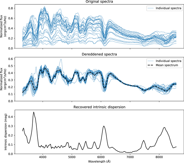
Figure 4. Comparison of the diversity of spectra at maximum light before and after dereddening. Top: a sample of the original rest-frame spectra of SNe Ia in our sample estimated at maximum light. Middle: the same spectra after estimating and removing the residual brightness and extinction relative to a mean spectrum following the RBTL procedure in Section 4.1. The estimated mean spectrum is shown with a dashed black line. Bottom: the estimated residual intrinsic dispersion η(λk ) from the RBTL procedure.
Download figure:
Standard image High-resolution imageThe Ca ii H&K lines, the Ca ii IR triplet, and the Si ii 6355 Å feature are the locations in the spectra of SNe Ia with the largest intrinsic dispersions. Interestingly, there are several regions of the spectra that are blanketed by lines but that still show relatively low intrinsic dispersion. From 3900 Å to 5900 Å, the spectra of SNe Ia show a variety of absorption lines, but the intrinsic diversity is recovered to be ∼0.08 mag at most wavelengths, with the exception of a handful of stronger lines that introduce diversity at up to 0.13 mag.
This model is effectively using the intrinsic diversity of SNe Ia to weight each wavelength when determining how to fit for the brightness and extinction of each SN. Hence, the lines with strong diversity are deweighted, and the model effectively “reads between the lines” to estimate the brightness and extinction.
5. A Nonlinear Model of the Intrinsic Variability of SNe Ia
Using the RBTL model, we have dereddened spectra of each SN Ia at maximum light with extrinsic contributions from distance uncertainties and interstellar dust removed. The remaining variability between these spectra can be interpreted as the intrinsic diversity of SNe Ia. In this section, we show that the intrinsic diversity is inherently nonlinear, and we build a nonlinear parametric model of the intrinsic diversity of SNe Ia.
5.1. Manifold Learning
The process of recovering a low-dimensional nonlinear parameter space from high-dimensional observations is referred to as “manifold learning.” Manifold learning has been shown to be very effective for constructing nonlinear parameterizations of the spectra and light curves of astronomical objects (Richards et al. 2009, 2012; Daniel et al. 2011; Matijevič et al. 2012; Sasdelli et al. 2016). A major challenge with nonlinear dimensionality reduction is that any transformation of a given parameterization is an equally valid parameterization. Many different manifold learning techniques exist, each of which imposes different assumptions and constraints on the recovered parameterization. Our goal is not to find an “optimal” parameterization of SNe Ia (which is not well defined), but instead, one that is useful for cosmological applications.
For this analysis, we choose to construct a parameterization of SNe Ia that preserves the spectral distances between twin SNe as described in F15. We define the spectral distance γij between two SNe Ia labeled i and j as
Our goal is to construct a parameterization of SNe Ia where the Euclidean distance between the coordinates of any two twin SNe Ia is equal to the spectral distance between those two SNe Ia. We do not require that the spectral distances of non-twins be preserved.
To accomplish these goals, we make use of the Isomap algorithm from Tenenbaum & Silva (2000). This algorithm is designed to embed points from a high-dimensional space into a low-dimensional one while preserving the distances between nearby points in the high-dimensional space. By using the spectral distance of Equation (11) as the distance measure for the Isomap algorithm, we will therefore generate an embedding that preserves the distances between twin SNe Ia.
The Isomap algorithm proceeds as follows. First, for each SN Ia, we find its K nearest neighbors using spectral distances. For each pair of SNe Ia in the sample, we then find the shortest path between the two SNe Ia passing through pairs of neighbors. We calculate the “geodesic distance” for each pair of SNe Ia as the sum of spectral distances between neighbors along each step in this path. After computing the geodesic distances between each pair of SNe Ia, we obtain a distance matrix. To generate an embedding, we center the distance matrix and compute its eigendecomposition (see Tenenbaum & Silva 2000 for details). For a D-dimensional embedding, we keep the D eigenvectors of the centered distance matrix with the largest eigenvalues. Each eigenvector then corresponds to a “component” of the embedding and captures a distinct mode of variability of SNe Ia. The values of the eigenvectors are the “coordinates” of each SN Ia within the embedding.
The Isomap algorithm has two parameters that must be set to produce an embedding: the number of neighbors K, and the dimensionality D of the embedding. As will be discussed in Section 5.5, the number of neighbors K does not have a major impact on the resulting embedding, and for a range of different values tested between ∼6 and 50, we obtain nearly identical embeddings. We choose to use 10 neighbors for the rest of our analysis. We will discuss the dimensionality of SNe Ia in Section 5.3.
The Isomap algorithm generates a low-dimensional embedding of SNe Ia, but it does not produce a model of the spectrum of an SN Ia given its coordinates in the embedding. Instead, to do this we use GP regression to model the spectra as a function of the Isomap coordinates. The details of this model are described in the Appendix. We use a separate GP model for each wavelength, and we optimize the hyperparameters of each GP independently.
5.2. Sample for Manifold Learning Analyses
For some of the SNe in our sample, the uncertainty on the spectrum at maximum light is comparable to the recovered intrinsic dispersion η(λk ). The Isomap algorithm is unable to take this uncertainty into account, so if spectra with large uncertainties are included in our analysis, we could confuse intrinsic diversity with the uncertainty in our estimate of the spectrum at maximum light. To mitigate this, we remove any SNe at this stage of the analysis whose uncertainties on the spectrum at maximum light are large compared to the intrinsic dispersion. We choose to require that the total measurement variance of the estimate of the spectrum at maximum light be less than 10% of the total intrinsic variance of SNe Ia. Choosing this fractional variance threshold requires somewhat of a trade-off: with better-measured spectra, we could potentially recover more components of the intrinsic dispersion, but a stricter threshold reduces the number of SNe Ia in the sample and thus our ability to reconstruct the parameter space. Out of the original sample of 203 SNe Ia, 173 SNe Ia have uncertainty on their spectrum at maximum light that passes this stringent fractional variance threshold. As will be shown in Section 5.5, whether this cut is applied has almost no effect on the embedding coordinates for the SNe Ia that pass it.
Note that in the RBTL analysis we included the estimates of the uncertainties for the spectra at maximum light, so the spectra that were cut due to the fractional variance threshold will not have a major impact on the RBTL analysis. We retrained the RBTL model on only the spectra that pass the uncertainty of the spectrum at the maximum light requirement and found that the changes were negligible (the estimated brightnesses change by <0.005 mag). As a result, we choose to use the RBTL model trained on all of the spectra for further analysis.
5.3. Dimensionality of the SN Ia Population at Maximum Light
We use the Isomap + GP model to investigate the dimensionality of SNe Ia. For a given number of Isomap components D, we examined what fraction of the variance is explained by the model. The results of this procedure are shown in Figure 5. We find that the first three components of the Isomap + GP model each explains a significant fraction (49.3, 26.2, and 11.1% respectively) of the total variance, and together, they explain 86.6% of the total variance. Measurement uncertainty accounts for 2.9% of the remaining variance for this sample, so our model explains 89.2% of the intrinsic variance when this is taken into account. Additional components beyond the third do not explain a significant amount of the remaining variance.
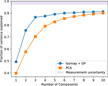
Figure 5. Fraction of the intrinsic variance of SNe Ia explained by different models. We show the results for both the nonlinear Isomap + GP model and a linear PCA-based model. The shaded area at the top of the plot corresponds to the fraction of variance explained by measurement noise.
Download figure:
Standard image High-resolution imageFor comparison purposes, we also perform a linear PCA decomposition of the same data. We find that the linear model requires seven components to explain as much of the variance as our three-component nonlinear model, which supports our claim that there is a significant amount of nonlinear variability in the spectra of SNe Ia.
We show the unexplained dispersion as a function of wavelength in Figure 6. After the RBTL procedure, the residual dispersion is ∼0.3 mag for the Ca ii and Si ii features. In contrast, with the three-component Isomap + GP model, there is less than 0.1 mag of residual dispersion at the wavelengths associated with these features, and the dispersion is less than 0.05 mag at almost all wavelengths. Again, adding components beyond the third has a negligible effect on the intrinsic dispersion.
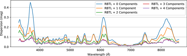
Figure 6. Residual intrinsic dispersion in the spectra of SNe Ia for Isomap + GP models with different numbers of components.
Download figure:
Standard image High-resolution imageAlternatively, we look at how well the spectral distances from Equation (11) are preserved in the embedding. We find that the Euclidean distances between two SNe Ia in the Isomap embedding have Pearson correlations with the F15 spectral distances of 0.77 for one component, 0.90 for two components, and 0.95 for either three or four components with very little improvement if additional components are added. With at least three components, we are therefore able to accurately preserve the spectral distances (and thus twin pairings) of F15.
Sasdelli et al. (2016) previously showed that deep learning can produce a nonlinear four-dimensional representation of SNe Ia. However, their analysis modeled the derivatives of the spectra in wavelength rather than modeling the spectra directly and did not include an explicit model of how spectra vary near maximum light or a means of measuring the brightness and color of a spectrum (which is necessary for cosmological applications). Because we explicitly model the extrinsic contributions to the spectrum, our model is able to explain significantly more of the variance in the spectra: with three components, we can explain 86.6% of the intrinsic variance compared to 82% with four components for the analysis of Sasdelli et al. (2016). Furthermore, the distances between two SNe Ia in the Twins Embedding capture the spectral distances of F15 while they have no meaning in the analysis of Sasdelli et al. (2016).
5.4. Reconstructing Spectra
We can use GPs to predict the spectrum of an SN Ia given its coordinates from the Isomap decomposition. To test how well our model would perform on new observations, we generate leave-one-out predictions where we condition the GP on spectra from all of the SNe Ia in our sample except for one SN Ia and predict the spectrum at the Isomap coordinates of the remaining SN Ia. Results of this procedure for three SNe Ia are shown in Figure 7. In this plot, we show the results for a “normal” SN Ia, a 91T-like SN Ia (Filippenko et al. 1992b), and a 91bg-like SN Ia (Filippenko et al. 1992a). We find that the three-component model is able to predict accurate spectra for the full range of SNe Ia including 91T-like and 91bg-like SNe Ia.
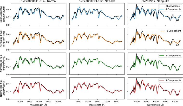
Figure 7. Examples of the leave-one-out Isomap + GP model predictions for SNe Ia with different numbers of components. The original observations are shown in black, while the model is shown in color. Each column corresponds to a different SN Ia. The first row shows the results of applying the RBTL model to capture brightness and color. Subsequent rows show the Isomap + GP model for different numbers of components.
Download figure:
Standard image High-resolution imageThere is still a small amount of residual dispersion after applying any of these models. To study this, we performed leave-one-out predictions for all of the SNe Ia in our sample and evaluated the correlation matrix of the residuals. The results of this procedure are shown in Figure 8. For the base RBTL model (left panel of Figure 8), we see a strong off-diagonal structure in the correlation matrix implying that the residuals at different wavelengths are highly correlated. In contrast, for the three-component Isomap + GP model (right panel of Figure 8), there is very little correlation between different wavelengths. This implies that the remaining variance is mostly uncorrelated across wavelengths and explains why adding additional components does little to improve the model.
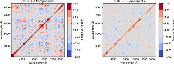
Figure 8. Correlation matrix of the residuals of spectra of SNe Ia with different models. Left panel: correlation matrix for the RBTL model. Right panel: correlation matrix for the three-component Isomap + GP model. We find that a three-component Isomap + GP model is able to capture the vast majority of the variance that is correlated across different wavelengths.
Download figure:
Standard image High-resolution imageWe conclude that a three-dimensional embedding is sufficient to explain the vast majority of the intrinsic diversity of SNe Ia at maximum light (along with extrinsic contributions from dust and brightness removed in Section 4). As this embedding was effectively constructed using pairs of twin SNe Ia, we refer to it hereafter as the “Twins Embedding.” We label the three components of the Twins Embedding ξ1, ξ2, and ξ3. The RBTL parameters and coordinates of each SN Ia in the Twins Embedding can be found in Table 3.
5.5. Stability of the Model
As described in Section 5.1, nonlinear dimensionality reduction is challenging because there is in general no unique solution. We investigated how stable the Twins Embedding is by making various modifications to the input data set and applying our algorithms to generate variants on the embedding. In general, there is no guarantee that the recovered embedding will be axis-aligned with our original one, especially if we modify the binning of the spectrum since that will change the weights of different regions. To perform a robust quantitative comparison, we fit a GP model to predict the coordinates in the original embedding from the coordinates in some alternative embedding. We use the same GP model that was used to predict the flux of each spectrum across the Twins Embedding, the details of which can be found in the Appendix. For each variant, we calculate the fraction of variance that is explained by the GP model. The results of this procedure are shown in Figure 9.
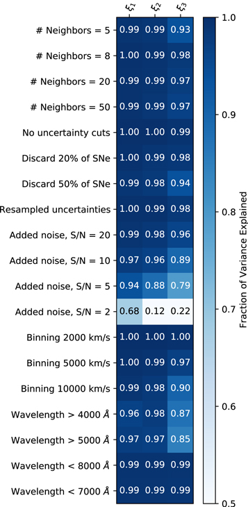
Figure 9. Comparison of how various modifications of the data set affect the Twins Embedding. For each modification, labeled on the left, we generate a three-component embedding and calculate the fraction of variance of the original Twins Embedding that can be explained by a transformation of the alternative embedding (see text for details).
Download figure:
Standard image High-resolution imageChanging the number of neighbors for the Isomap algorithm has very little effect on the recovered embedding for values between ∼5 and 50 neighbors. For fewer than five neighbors, we find that we are unable to recover the third component. This is likely due to the fact that using a small number of neighbors adds noise to the distance matrix. Removing the uncertainty cuts described in Section 5.2 has almost no effect on the recovered embedding. Similarly, randomly discarding 20% or 50% of the SNe Ia in the sample does not noticeably affect the embedding.
Our sample was selected to have very high signal to noise, so resampling the uncertainties of each spectrum has little effect on the recovered embedding. We find that we are able to degrade the spectrum down to an S/N of ∼5 per 1000 km s−1 before we start to see a degradation in the recovered embedding. Interestingly, we are able to bin the spectrum down to ∼10000 km s−1 before we see significant changes in the embedding, which corresponds to a very low-resolution spectrum (R ∼ 30).
Finally, we investigated how changing the wavelength range of our spectra from the baseline of 3300–8600 Å affects the recovered spectrum. Decreasing the cutoff wavelength at the red end has almost no effect on the embedding, but increasing the cutoff at the blue end does, with a significant degradation in the third component for cutoffs above ∼4000 Å. As discussed in detail in Nordin et al. (2018), there is a large amount of variability in the U band, particularly near the Ca ii H&K lines, and not having observations of this region of the spectrum significantly degrades the performance of our model.
6. Exploring the Intrinsic Diversity of SNe Ia
6.1. Components of the Twins Embedding
We now examine what effects each of the three components of the Twins Embedding has on the spectrum of an SN Ia. For each component, we calculate the median spectrum in 20 evenly populated bins of the coordinates for that component. We plot these median spectra in Figure 10. We find that each component captures a different smooth, nonlinear spectral sequence.
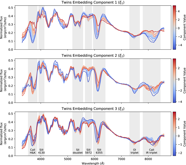
Figure 10. Effect of each of the components of the Twins Embedding on the spectra of SNe Ia at maximum light. For each component, we show the median spectrum in 20 evenly populated bins of the coordinates of that component. The spectra are colored according to their component value.
Download figure:
Standard image High-resolution imageThe first component of the Twins Embedding (ξ1) primarily affects the pseudo-equivalent widths (pEWs) of the Ca ii features. This component maps out a full spectral sequence of the changing pEW of the Ca ii H&K feature, and a similar spectral sequence is seen for the Ca ii IR triplet. Additionally, ξ1 shows a spectral sequence for the Si ii 6355 Å feature. This component is the only one that has a major impact on the emission profile of this feature and appears to be capturing diversity in both the optical depth and line velocity of the Si ii 6355 Å feature. ξ1 has very little effect on the depth of the Si ii 5972 Å feature that is typically associated with the width of the light curve.
The second component (ξ2) primarily affects the pEWs of the Si ii lines. A spectral sequence is identified in the Si ii 4130 Å, Si ii 5972 Å, and 6355 Å features. Interestingly, this component directly changes the depths of these lines without having a major effect on the line velocities themselves. ξ2 also has a large effect around 3700 Å that appears to be due to a set of Si ii lines at rest-frame wavelengths between 3853 and 3863 Å. This component does not appear to affect the Ca ii H&K absorption typically associated with these wavelengths, and by comparing with ξ1, we can see that the Twins Embedding cleanly separates two modes of variability in this wavelength range. ξ2 has a very complex spectral sequence for redder wavelengths, spanning both the O i and Ca ii features.
The third component ξ3 primarily affects the ejecta velocity profiles of the SN. This component identifies a spectral sequence in the velocity of the S ii doublet feature near 5400 Å and in the velocity profile of the Si ii 6355 Å feature. Interestingly, ξ3 seems to capture an overall shift in velocity in the emission profile: as this component is varied, we see the full absorption profile shift in wavelength for both the S ii doublet and the Si ii 6355 Å feature. This contrasts with ξ1, which also alters the observed line velocity of these emission features by increasing the optical depth of these elements at larger velocities. Similar effects are seen for the velocities of many other lines in the spectra. ξ3 does not have a major effect on any of the line depths in the spectrum. Interestingly, we see a sequence in the pseudo-continuum level around the Si ii 5972 Å feature that does not affect the pEW of this feature.
6.2. Recovering Other Indicators of Intrinsic Diversity
If the Twins Embedding truly captures all of the observable intrinsic diversity of SNe Ia, then we would expect to be able to recover any indicator of intrinsic diversity of SNe Ia from some transformation of the Twins Embedding. We tested this hypothesis by training GP models to predict a wide variety of indicators from the Twins Embedding, and then by measuring the fraction of the variance in those indicators that is explained by the GP models.
First, we extracted the pEWs and line velocities of the Ca ii H&K feature and several of the Si ii features using the methodology described in Chotard et al. (2011) on each of the dereddened spectra. For SNe Ia that were included in the U-band analysis of Nordin et al. (2018), we include their spectral indicators uNi, uTi, uSi, and uCa at maximum light, and we also include the uCa measurement prepeak and uTi measurement postpeak that the authors show affect standardization. For SNe Ia that were included in the SUGAR analysis of Léget et al. (2020), we include their SUGAR coordinates. Similarly, for SNe Ia that were included in the SNEMO analysis of Saunders et al. (2018), we include their SNEMO7 coordinates. Finally, we compare our embedding to the SALT2 x1 values measured as described in Section 2. As SALT2 is not able to accurately model all of the peculiar SNe Ia that we have included in our sample, for this comparison, we reject SNe Ia with bad SALT2 fits where the normalized median absolute deviation (NMAD) of the SALT2 model residuals is more than 0.12 mag or where more than 20% of the SALT2 model residuals have an amplitude of more than 0.2 mag.
We use the same GP model that was used to predict the flux of each spectrum over the Twins Embedding. The details of this GP model can be found in the Appendix. When available, we include the measurement uncertainties of the indicators in the GP model. In Figure 11, we show the results of this procedure. We find that the Twins Embedding captures the majority of the diversity in all of these indicators, with 68%–94% of the variance explained depending on the indicator. We verified with leave-one-out GP predictions that we are able to perform out-of-sample predictions of each of these indicators within the quoted accuracies.
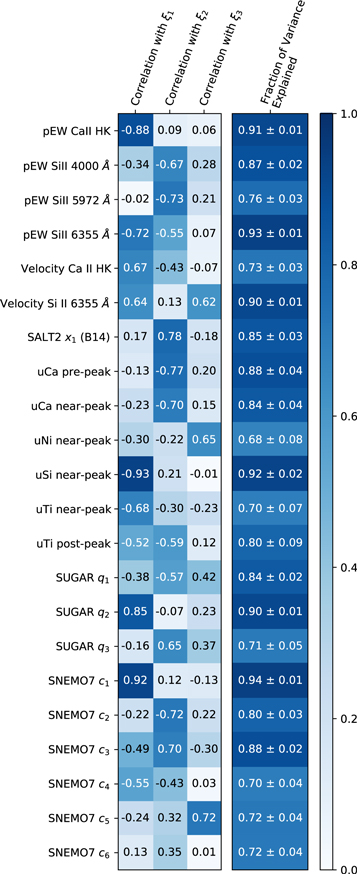
Figure 11. Recovery of various indicators of intrinsic diversity from the Twins Embedding. In the first three columns, we show the Pearson correlation between each indicator and one of the components of the Twins Embedding. In the final column, we show the fraction of variance of each indicator that can be explained using a transformation of the Twins Embedding. All of these previously established indicators can be recovered with high accuracy from the three-dimensional Twins Embedding.
Download figure:
Standard image High-resolution imageAdding an additional component to the Twins Embedding does not significantly improve the ability to recover any of these indicators while removing the third component ξ3 significantly decreases performance, further confirming that three dimensions are required to capture the diversity of SNe Ia. Interestingly, with transformations of the Twins Embedding, we are able to recover the majority of the variance in each of the components of the SNEMO7 model of Saunders et al. (2018). Given the location of an SN Ia in the three-dimensional Twins Embedding, we can therefore predict its location in the six-dimensional SNEMO7 parameter space with high accuracy. Our results imply that the six components of SNEMO7 are not all independent and can be captured by a three-dimensional submanifold. SNEMO7 is a linear model, and this is consistent with the results that we found for a simple linear model in Section 5.3. Note that the SNEMO7 parameter space was constructed using full spectral time series of SNe Ia while the Twins Embedding was constructed using only information at maximum light. These results then suggest that the vast majority of the information in the spectral time series of SNe Ia is captured at maximum light.
In our comparison to the SUGAR model (Léget et al. 2020), we find that we are able to reproduce the first two components of the SUGAR model with high accuracy and the majority of the variance of the third SUGAR component. Hence, the SUGAR parameter space is very similar to the Twins Embedding despite having been constructed very differently (a linear decomposition of spectral features). We reran our algorithm to calculate the fraction of explained variance for each indicator using a transformation of the SUGAR parameter space rather than a transformation of the Twins Embedding. We find that both parameterizations of SNe Ia are able to explain similar fractions of the variance for most of the indicators that we examined. However, the SUGAR model performs significantly worse on the U-band features of Nordin et al. (2018). For example, it is only able to recover 42% of the variance of the uNi indicator at maximum light compared to 71% for the Twins Embedding using the same set of SNe Ia. This can be explained by the fact that the SUGAR model was trained using only a specific set of spectral features, and is potentially missing information that is not captured in those spectral features. On the other hand, the Twins Embedding was trained using the entire spectrum at maximum light. Furthermore, the SUGAR analysis removed “outlier SNe Ia” that are not well described by a linear model while the Twins Embedding includes all of these SNe Ia because it is not restricted to linear variability.
6.3. Comparison to the Branch Classification Scheme—Diversity of Core Normal SNe Ia
The spectra of SNe Ia near maximum light are often labeled in the literature using the “Branch classification scheme” (Branch et al. 2006, hereafter B06). In this classification scheme, the spectra of SNe Ia are subdivided into four classes based on the pEWs of the Si ii 5972 and 6355 Å absorption features. As has been previously shown for large samples of spectra of SNe Ia (e.g., Blondin et al. 2012), the Branch classifications do not identify distinct subtypes of SNe Ia, and we find a continuous distribution across all of the label boundaries.
We compare the Branch classifications to our Twins Embedding in Figure 12. We find that the first two components of the Twins Embedding (ξ1 and ξ2) cleanly separate the different Branch classes from each other: with a set of cuts in the Twins Embedding, we would be able to recreate the Branch classification scheme nearly perfectly. There is some overlap at the border of each class due to uncertainties in the pEW measurements used for the Branch classification. Interestingly, while core normal SNe Ia lie in a tight cluster in the parameter space used for Branch classifications, they are spread over a fairly large region of the Twins Embedding.
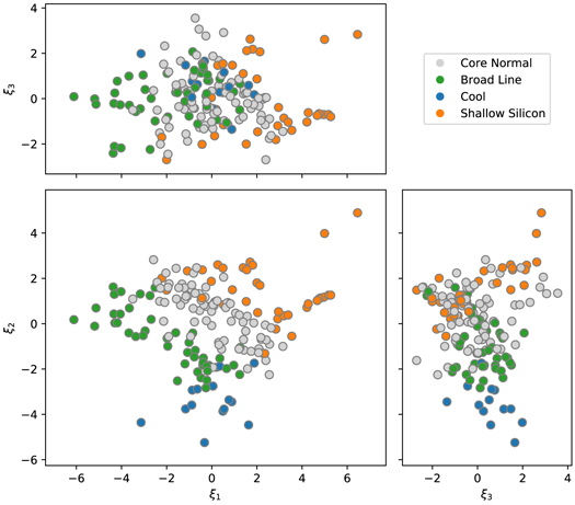
Figure 12. Comparison of the Branch classifications B06 to the Twins Embedding. We find that with the first two components (ξ1 and ξ2) we are able to cleanly recover the Branch classification labels.
Download figure:
Standard image High-resolution imageThe Twins Embedding thus implies that there is significant spectral diversity among core normal SNe Ia. To probe this claim, we calculated the median spectrum for core normal SNe Ia in ten equally populated bins of ξ1. The results of this procedure are shown in Figure 13. All of these median spectra have similar pEWs for the Si ii 6355 Å absorption feature and have a small pEW for the Si ii 5972 Å feature, per the definition of a core normal SN. However, the pseudo-continuum level near the Si ii 5972 Å feature varies quite dramatically between the different median spectra. As analyses such as B06 focused only on the pEW and ignore the pseudo-continuum level, they were not able to identify this difference. We also see large differences for these spectra near 3800 Å, which we associate with a set of Si ii lines between 3853 and 3863 Å. These differences were not seen in B06 due to a lack of spectral coverage. Finally, we see a spectral sequence for an absorption feature near 8000 Å. This difference was identified in B06 for SN 2001el and was suggested to be due to high-velocity Ca ii. Hence, with only the first two components, the Twins Embedding is able to reproduce the Branch classification scheme and is able to identify additional diversity that is not solely limited to the pEWs and velocities of different lines.
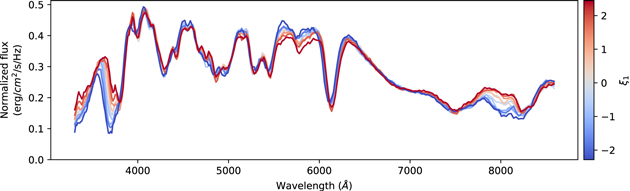
Figure 13. Comparison of the spectra of core normal SNe as a function of the first component of the Twins Embedding (ξ1). We show the median spectrum for 10 equally populated bins of ξ1. We find that the Twins Embedding identifies significant differences between core normal SNe Ia. Note that there are large differences in the pseudo-continuum level near the Si ii 5972 Å feature that will not be captured by analyses measuring only pseudo-equivalent widths or line velocities of this feature.
Download figure:
Standard image High-resolution image6.4. Connecting Subtypes of SNe Ia
One major open question about SNe Ia is whether there exist subtypes of SNe Ia, perhaps from different progenitor channels. To look for signs of such subtypes, we examine the distribution of the SNe Ia in the Twins Embedding as seen in, e.g., Figure 12. For this sample of SNe Ia, we do not see any evidence of large-scale bimodality in the recovered parameter space: the core of the parameter space is well populated and appears to be continuously filled. Note that we constructed the Twins Embedding using nonlinear dimensionality reduction, with the goal of preserving the spectral distances between “twin” SNe Ia from F15. The distances between points in the embedding should be meaningful because we are capturing the vast majority of the variance, as shown in Section 5.3, but the exact shape of the distribution of SNe Ia in the embedding will depend on the algorithm used and should not be overinterpreted.
The Twins Embedding includes all SNe Ia, including ones that are typically referred to as “peculiar.” We identified where the peculiar subclasses of 91bg-like (Filippenko et al. 1992a), 91T-like (Filippenko et al. 1992b), and 02cx-like SNe Ia (Li et al. 2003) are located in the Twins Embedding. We use the labeling of peculiar SNe Ia for the SNfactory sample from Lin et al. (2021). The results of this procedure can be seen in Figure 14.
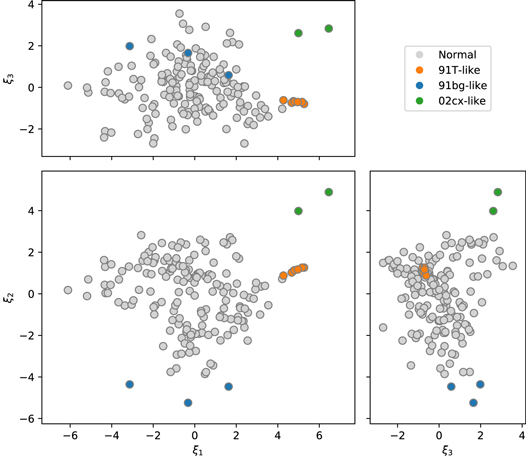
Figure 14. Location of peculiar SNe Ia in the Twins Embedding.
Download figure:
Standard image High-resolution imageWe find that all three of these kinds of peculiar SNe Ia lie at the edges of the Twins Embedding. They are easily separable from the rest of the sample using their coordinates in the Twins Embedding. There are seven 91T-like SNe Ia in our sample that are all tightly clustered at large values of ξ1. The dereddened spectra of the 91T-like SNe Ia are all nearly identical, which explains why they lie in such a small region of the Twins Embedding. The three 91bg-like SNe Ia lie at very low values of ξ2 with a significant spread in ξ1. The two 02cx-like SNe Ia in our sample are separated from the rest of the sample in all of the Twins Embedding components.
One way to probe whether different SNe Ia are from the same physical processes is to test whether we can find a set of other SNe Ia whose spectra form a continuous sequence from the first spectrum to the second. If such a sequence can be found, then it suggests that the observed differences between those two SNe Ia are due to some continuous underlying physical parameter rather than being due to discrete processes. By selecting SNe Ia that lie along a path in the Twins Embedding, we can identify such a sequence between any two SNe Ia. In panel (A) of Figure 15, we show an example of this procedure by identifying a set of eight SNe Ia that are evenly spaced between the Twins Embedding coordinates of PTF 11kjn (a 91bg-like SN Ia) and SNF 20080522–000 (a 91T-like SN Ia). At each step in this sequence, the adjacent SNe Ia are “twins” according to the definition of F15, except for the initial pairing of PTF 11kjn to SN 2013bs whose “twinness percentile” of 29% is slightly above the threshold of 20% defined in F15 due to the low density of SNe Ia in this region of the parameter space. This sequence of SNe Ia is consistent at all wavelengths: the spectral features evolve continuously when traversing the sequence of spectra, although the changes in the spectral features are highly nonlinear. We are able to produce similar sequences between any two 91bg-like, 91T-like, or “normal” SNe Ia. This suggests that all of these SNe Ia may come from the same underlying process and that their diversity could be explained by variations in some continuous underlying parameters.
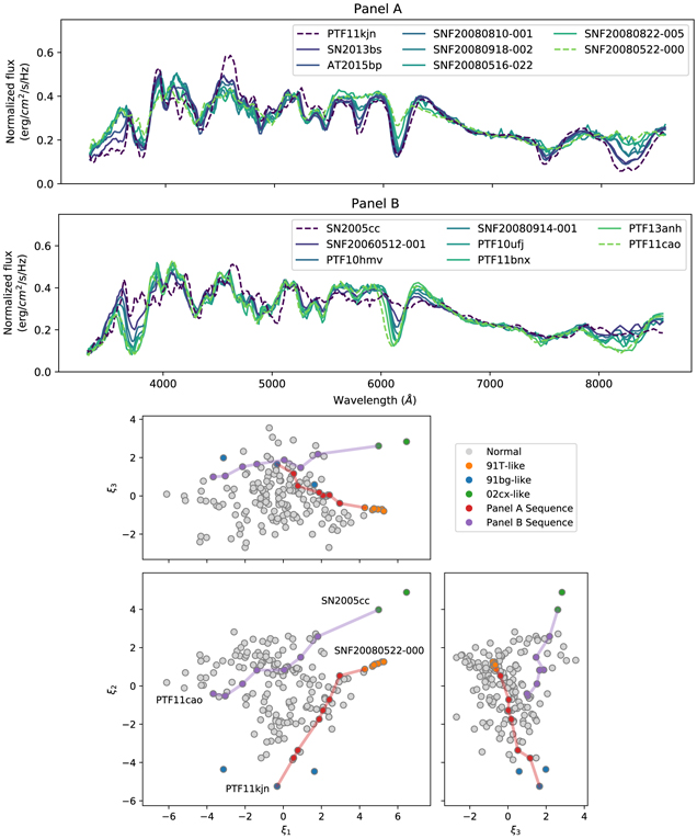
Figure 15. Sequences of SNe Ia near evenly spaced coordinates in the Twins Embedding. Panel (A): a sequence between the 91bg-like PTF 11kjn and the 91T-like SNF 20080522–000. These SNe Ia map out a continuous spectral sequence at all wavelengths, and each pair of adjacent SNe Ia in the sequence is a set of “twins” according to the definition of F15 except for PTF 11kjn and SN 2013bs that are slightly above the threshold. Panel (B): a sequence between the 02cx-like SN 2005cc and the “normal” PTF11cao. SN 2005cc has large spectral differences relative to its closest neighbor, SNF 20060512–001, and does not follow the spectral sequence that is established at most wavelengths. The bottom panels show the Twins Embedding coordinates of the SNe Ia in each of these sequences in red and purple, respectively.
Download figure:
Standard image High-resolution imageOn the other hand, we find that we are unable to identify continuous sequences of SNe Ia between 02cx-like SNe Ia and the rest of the sample. An example of an attempt at such a sequence is shown in panel (B) of Figure 15. SN 2005cc has large spectral differences relative to the next point in the sequence, SNF 20060512–001, and this pair falls into the 64th percentile of F15 twinness, which is worse than a random matching. The spectral differences that are seen do not follow the established sequence from the other SNe Ia, especially between 3800 and 5000 Å. Similar results are found for the other 02cx-like SN Ia in our sample, SN 2011ay. This could be suggestive of a different underlying process, but it is difficult to make definitive conclusions with our small sample of only two 02cx-like SNe Ia because we could simply be lacking intermediate SNe Ia in our sample.
7. Conclusions
In this work, we showed how the diversity of the spectra of SNe Ia at maximum light can be decomposed into its various components. In Section 3, we showed how we can estimate the spectrum at maximum light for an SN Ia using spectra within five days of maximum light using a model of the differential time evolution of SNe Ia near maximum light. This method is completely agnostic to extrinsic sources of diversity such as dust extinction or distance uncertainties. We find that 84.6% of the variance in the evolution of SNe Ia near maximum light is common to all SNe Ia.
In Section 4, we developed a new technique to estimate extrinsic contributions to the spectra of SNe Ia at maximum light that we call “Reading Between the Lines” (RBTL). This technique effectively uses the regions of the spectra of SNe Ia between major spectral features where there is little intrinsic variability to estimate the extrinsic effects on the spectrum such as the overall brightness and reddening due to dust. We find that SNe Ia are incredibly homogeneous in regions of the spectra between major spectral features. For example, for the region between 6600 and 7200 Å, we find an intrinsic dispersion of only ∼0.02 mag. After the RBTL procedure, we are left with a set of dereddened spectra of SNe Ia at maximum light that only have intrinsic diversity remaining.
In Section 5, we showed how manifold learning can be used to map out the intrinsic diversity of SNe Ia by building a parameter space from pairs of twin SNe Ia that we call the Twins Embedding. We find that a three-dimensional parameterization captures 89.2% of the intrinsic diversity of SNe Ia at maximum light. The three components of the Twins Embedding primarily affect the Ca ii features, the Si ii features, and the photosphere expansion velocities, respectively. From this parameter space, we are able to recover the majority of the variance in a wide range of previously established indicators of intrinsic diversity of SNe Ia. We are able to reproduce the classifications of Branch et al. (2006) with the first two components of the Twins Embedding and can also identify additional diversity among core normal SNe Ia that are not captured in the classification of Branch et al. (2006).
This analysis included the full range of SNe Ia observed by the SNfactory, including the so-called “peculiar” SNe Ia. We showed that we can use the Twins Embedding to identify spectral sequences between any two SNe Ia, including 91bg-like and 91T-like SNe Ia but excluding 02cx-like SNe Ia. This suggests that the diversity of these SNe Ia could be due to continuous variation in some underlying physical processes rather than being due to different discrete processes, although we cannot make definitive conclusions with the limited size of our current data set.
One limitation of our analysis is that we performed a sequential decomposition of the diversity of spectra at maximum light rather than a simultaneous one. This will introduce additional uncertainty into the model, but we used very high-S/N observations for this analysis so each step of the model is very well constrained. Another potential concern is that our model is not flexible enough to capture the full diversity of SNe Ia. For example, the phase evolution near maximum light likely varies for SNe Ia at different locations in the Twins Embedding. This will not affect our analysis, as discussed in Section 3, because we modeled the unexplained dispersion and found that it is very small compared to the effects that we model in the rest of the analysis. In a future analysis, we plan on developing a hierarchical model that can simultaneously fit all of the components of the model described here.
This analysis only considered spectra of SNe Ia at maximum light. There could be additional intrinsic diversity in the light curves of SNe Ia that is not captured in the spectra at maximum light, although F15 showed that the twinning procedure performs as well using only spectra near maximum light as it does with the full spectral time series, and we are able to recover the majority of the variance in the SNEMO7 components of Saunders et al. (2018) that were trained on the full spectral time series. The range of additional intrinsic diversity at other phases could be probed by comparing the full time series of SNe Ia at similar locations in the Twins Embedding. A similar concern is diversity in the extrinsic variability of SNe Ia, such as variability in the dust RV . As discussed in Section 4.1, the construction of the Twins Embedding is effectively insensitive to RV variation. However, RV variation could be probed by comparing SNe Ia at similar locations in the Twins Embedding.
In Paper II, we show how the Twins Embedding can be used to improve the standardization of SNe Ia. To summarize its conclusions, there is significant diversity in the luminosity of SNe Ia that is not explained by the light-curve width and color but that can be identified using Twins Embedding. Taking this additional information about intrinsic diversity into account reduces uncertainties in the distance estimates to SNe Ia and reduces correlations with host-galaxy properties.
All of the code used in this analysis is publicly available at https://doi.org/10.5281/zenodo.4670772, and the data are available on the SNfactory website at https://snfactory.lbl.gov/snf/data/.
We thank the technical staff of the University of Hawaii 2.2-m telescope and Dan Birchall for observing assistance. We recognize the significant cultural role of Maunakea within the indigenous Hawaiian community, and we appreciate the opportunity to conduct observations from this revered site. This work was supported in part by the Director, Office of Science, Office of High Energy Physics of the US Department of Energy under contract No. DE-AC025CH11231. Additional support was provided by NASA under the Astrophysics Data 1095 Analysis Program grant 15-ADAP15-0256 (PI: Aldering). Support in France was provided by CNRS/IN2P3, CNRS/INSU, and PNC; LPNHE acknowledges support from LABEX ILP, supported by French state funds managed by the ANR within the Investissements d’Avenir program under reference ANR-11-IDEX-0004-02. Support in Germany was provided by DFG through TRR33 The Dark Universe and by DLR through grants FKZ 50OR1503 and FKZ 50OR1602. In China, support was provided by Tsinghua University 985 grant and NSFC grant No. 11173017. We thank the Gordon and Betty Moore Foundation for their continuing support. This project has received funding from the European Research Council (ERC) under the European Unions Horizon 2020 research and innovation program (grant agreement No. 759194–USNAC).
Appendix: Gaussian Process Regression
We use GP regression to model how different properties of SNe Ia vary across the Twins Embedding. A GP is a stochastic process over some set of continuous inputs where observations at any finite set of inputs follow a multivariate normal distribution. For a comprehensive discussion of GPs, see Rasmussen & Williams (2006). In our case, we use GPs to produce nonparametric models of how different properties of SNe Ia vary over the Twins Embedding.
We assume that the covariance between observations fi and fj at respective coordinates x i and x j can be described using the following function referred to as a “kernel”:
The first term of this equation is a Matérn 3/2 kernel that captures the covariance between observations at nearby coordinates with hyperparameters for the amplitude A and the length scale l. The second term captures uncorrelated variance for repeated observations at the same coordinates, with the intrinsic dispersion represented by the hyperparameter η.
We include an additional hyperparameter μ in our GP model representing a constant mean value. A set of observations f is then described by

For each property, we optimize the hyperparameters of the model to maximize the likelihood. We implement this model using the George package (Ambikasaran et al. 2015). The final model can then be used to estimate the value of the property at any location in the Twins Embedding by conditioning the GP on the observations of that property.