Abstract
In this paper, we collect a sample of stars observed both in LAMOST and Gaia, which have colors implying a temperature hotter than 7000 K. We train a machine-learning algorithm on LAMOST spectroscopic data which has been tagged with stellar classifications and metallicities, and use this machine to construct a catalog of blue horizontal branch stars (BHBs), together with metallicity information. Another machine is trained using Gaia parallaxes to predict absolute magnitudes for these stars. The final catalog of 13,693 BHBs is thought to be about 86% pure, with σ[Fe/H] ∼ 0.35 dex, and σG ∼ 0.31 mag. These values are confirmed via comparison to globular clusters, although a covariance error seems to affect our magnitude and abundance estimates. We analyze a subset of this catalog in the Galactic Halo. We find that BHB populations in the outer halo appear redder, which could imply a younger population, and that the metallicity gradient is relatively flat around [Fe/H] = −1.9 dex over our sample footprint. We find that our metal-rich BHB stars are on more radial velocity dispersion-dominated orbits (β ∼ 0.70) at all radii than our metal-poor BHB stars (β ∼ 0.62).
1. Introduction
Blue horizontal branch stars are reliable “standard candle” stars, commonly used for studying the Galactic halo (e.g., Greenstein & Sargent 1974; Beers et al. 1992; Yanny et al. 2000). They are helium-burning giants, which have evolved off the red giant branch (and as such, thought to be old, e.g., Hoyle & Schwarzschild 1955), with absolute magnitudes near to zero in a variety of optical bands. The anatomy of the horizontal branch begins at the cool end with the red horizontal branch (near the red clump), progresses blueward, through the RR Lyrae gap into the blue horizontal branch, and then falls off in magnitude down the extreme horizontal branch (see the review of Catelan 2009).
Owing to their low surface gravities, BHBs exhibit narrow spectral lines compared to main-sequence stars, and may be selected on that basis (Pier 1983; Flynn et al. 1994; Clewley et al. 2002). This variation in spectral line shape, near the absorption line series’ limits, also causes a net change in continuum flux, which may be exploited to select these types of star, based on filter colors (e.g., Bell et al. 2010; Deason et al. 2011; Vickers et al. 2012).
While photometric studies of BHB stars allow observations extending to great distances (e.g., the Magellanic Clouds, in Belokurov & Koposov 2016, or the halo to hundreds of kpc, in Nie et al. 2015; Deason et al. 2018; Fukushima et al. 2018, 2019; Thomas et al. 2018), they suffer worse contamination (∼30%; Sirko et al. 2004; Bell et al. 2010) than spectroscopic studies (<10%; Xue et al. 2008; Ruhland et al. 2011; although impressive progress has been made using specialized photometric filters; see e.g., Starkenburg et al. 2019, who find their photometrically selected sample of BHBs to be not only over 90% pure, but also more than 90% complete). 4 Spectroscopy also unlocks the sixth-phase coordinate, via radial velocity measurements.
Unfortunately, BHB stars’ hot temperatures (>7000 K) necessitate special spectroscopic treatment (see e.g., the Sloan Digital Sky Survey pipeline, Lee et al. 2008, and the special A-star procedure implemented in Wilhelm et al. 1999), as compared to the standard pipeline, which is generally optimized for FGK dwarfs (e.g., Boeche et al. 2018; Lee et al. 2015); as such, specialized methods must be coded.
In recent years, however, spectroscopic analysis has benefited disproportionately from machine-learning techniques. Learning algorithms may use examples of data which have already been “labeled” with spectroscopic parameters to label new data, without the need for researchers to code specific procedures for different species of stars by hand (e.g., “The Cannon,” in Ness et al. 2015, and the “Stellar LAbel Machine,” SLAM, in Zhang et al. 2020). This approach allows for many different types of stars to be reduced using a single, generalized, pipeline procedure, with the machine learning how to deal with various types of stars on the basis of previously reduced data.
Using such an approach, we will construct one of the largest spectroscopic samples of BHB stars to date, comprising almost 14,000 BHB candidates, which will be used to investigate the ancient history of the Milky Way.
BHBs have long been used to study the Milky Way halo. Their bright absolute magnitudes allow them to probe great distances, and their old ages are ideal for studying the canonical in situ halo. While the halo formation scenario has been more complicated in recent years, developing beyond the monolithic collapse theory of Eggen et al. (1962), to the current understanding of hierarchical formation (Searle & Zinn 1978; Helmi et al. 1999; Newberg et al. 2002), BHBs remain useful in research terms, as their accreted satellites often possess ancient BHB populations of their own.
This paper proceeds as follows: in Section 2, we describe the data to be classified and reduced, and go through how we assign classifications, metallicities, and absolute magnitudes to our data; in Section 2.6, we describe some “sanity checks” to double-check our reduced data (such as comparing pipeline values to globular cluster values); in Section 3, we describe our coordinate systems; in Section 4, we look over the chemistry, kinematics, and ages of our halo BHBs; we discuss our findings in Section 5, and conclude in Section 6.
1.1. Abbreviations and Notation
For this paper, we will use the following abbreviations: “BHB” is a blue horizontal branch star; “MSA” is a main-sequence A-type star 5 ; “XGB” indicates an extreme gradient-boosted (XGBoost) random forest algorithm, or a value which has been predicted by one; ϖ indicates Gaia parallax, or a value calculated from it; the subscript “0” indicates a photometric value which has been corrected using the full column extinction of Schlegel et al. (1998), with filter coefficients taken from Casagrande & VandenBerg (2018); an upper-case G will represent an absolute magnitude in the Gaia g band; “SNR” stands for signal-to-noise ratio.
2. Predicting Stellar Types, Metallicities, and Absolute Magnitudes with XGBoost
2.1. Data
Our BHB catalog will be constructed from data collected by the Large Area Multi-Object Spectroscopic Telescope (LAMOST; Luo et al. 2015). This telescope, located at Xinglong Station in Hebei Province, collects 4000 spectra per exposure, at a resolution of R ∼ 1800, and down to a magnitude of r = 19. As of data release 5, the survey contains about 9 million spectra in total.
The standard LAMOST pipeline (Wu et al. 2011) struggles to give accurate stellar parameters for stars hotter than ∼7000 K, as it is optimized for the more prevalent main-sequence stars. Since we are interested in BHB stars, which have temperatures up to 10,000 K, we will need to process the spectra ourselves.
Here, 155,549 LAMOST spectra are selected as BHB candidates having Gaia DR2 (Lindegren & Perryman 1996; Gaia Collaboration et al. 2018) colors bluer than (bp-rp) = 0.5, roughly corresponding to 7000 K. These spectra are normalized following Boeche et al. (2018).
2.2. Foundation
The fundamental spectral difference between BHB stars and the main contaminants in this spectral color regime (main-sequence A stars and blue stragglers, quasars, and white dwarfs) is the presence of hydrogen absorption lines (which are instead emission lines in quasar spectra), which are narrow due to the low surface gravity of giant BHBs, as compared to those of other stellar contaminants. See, for example, Vickers et al. (2012), Figures 7 and 8, and Yanny et al. (2000), Figure 8.
Previous works frequently relied on fitting line profiles to differentiate BHBs from different species of stars by their surface gravity (e.g., Clewley et al. 2002; Sirko et al. 2004; Xue et al. 2008). However, with modern machine-learning tools becoming readily available and easily accessible on personal computers, we opt to classify our BHB stars using a data-driven algorithm.
The benefit of using a machine-learning framework to classify BHB stars lies in the fact that we can readily use information from the entire spectra, whereas prior line-fitting methods rely on carefully selecting the wavelength ranges of individual lines. The absorption features follow profiles 6 which merge into the continuum, or even into each other, as is the case in stars with exceptionally strong surface gravities, such as white dwarfs. Utilizing the entire spectra avoids problems associated with mis-selecting profile extents and shape profiles, and allows more spectral information, such as non-targeted, incidental lines, to be utilized.
The difficulty of using a machine learning-supervised algorithm is that we require a training set which is regarded as “true” for the machine to learn from. The supervised algorithm will consider a training dataset which is in the same data format as the data to be classified, (i.e., LAMOST spectra), with tags for the classes (i.e., “BHB,” “not-BHB”), and thereby construct a mathematical equation 7 through which the data may be passed to yield a numerical value. This numerical value may be a regressed value (as is the case when fitting a continuous metric, such as metallicity), or a 1-0 class value (as we are doing here for BHB, not-BHB).
This need for a training set means that a subset of the data must be processed and classified by hand before the bulk of the data may be classified by machine—it must be “supervised” by an intelligent actor. In this way, modern data-driven pipelines rest very directly on the shoulders of past researchers, who have painstakingly reduced subsets of these data by hand.
2.3. Training Data
The Century Survey of Brown et al. (2008) is a catalog of 2414 color-selected BHB candidates over 10% of the sky, based on the Two-Micron All Sky Survey (Skrutskie et al. 2006) in 12.5 ≤ J0 ≤ 15.5. This survey confirmed 655 of these candidates as “true” BHB stars. LAMOST has observed 573 of the 2414 candidates, and 213 of the 655 confirmed BHB stars (at SNRg,r,i > 10).
The catalog of Xue et al. (2008) took the Sloan Digital Sky Survey (York et al. 2000) spectra, and reprocessed ∼10,000 color-selected BHB candidates, using a specialized pipeline for hot stars. This yielded 2558 confirmed BHB stars. LAMOST has observed 833 of these 10,000 candidates, and 380 of the 2558 confirmed BHB stars (at SNRg,r,i > 10).
On the basis of these two surveys, we have a training set of 1,406 objects in LAMOST: 593 BHBs, and 813 not-BHBs. To prepare the data to be interpreted, we shift all the spectra to their rest wavelengths, according to their LAMOST radial velocity. Since the spectra are nonlinearly sampled in their observed wavelength (R = λ/Δλ ∼ 1800), the rest-wavelength spectra are sampled incongruently with each other. To be directly compared, the data must be sampled at the same rest wavelengths. This may be accomplished by binning the data, which loses information, but conserves computer resources, or by upsampling the data (linearly interpolating between the observed wavelengths at set points on a wavelength grid at a higher frequency than the original data), which conserves information, but becomes more computationally costly. We opt for the latter, with an upsampled grid every 0.84 Å, which is slightly more than one grid point per measurement at the blue end of the spectra, and more dense per measurement at the red end. Our grid extends from 3850 to 8900 Å, which is the maximal extent covered by all spectra in our dataset (at rest wavelengths). Note that this dataset is pre-cut to include only data with radial velocities of less than 1000 km s−1. 8
Our training sample, using data from Xue et al. (2008) and the Century Survey (Brown et al. 2008), contains 1,406 stars with BHBs making up 42%. For a full breakdown, see Table 1.
Table 1. The Makeup of Our Training Sets in the Full Sample, and in the 10% Parallax Error Sample
| Survey (Total/<10%ϖ error) | NFull | N10%ϖ | |
|---|---|---|---|
| Century (573/175) | BHB | 213 (37%) | 18 (10%) |
| MSA | 154 (27%) | 68 (39%) | |
| BHB/MSA | 47 (8%) | 4 (2%) | |
| subdwarf | 17 (3%) | 12 (7%) | |
| DA white dwarf | 8 (1%) | 8 (5%) | |
| None | 134 (23%) | 65 (37%) | |
| Xue (833/180) | BHB | 380 (46%) | 103 (57%) |
| MSA/BS | 453 (54%) | 77 (43%) | |
Download table as: ASCIITypeset image
2.4. The Machine
With our training data and data to be classified in hand, we return to the machine-learning problem. We utilize the extreme gradient boosting method (XGB 9 , Chen & Guestrin 2016). This modern machine-learning method is an optimized version of “gradient boosting” (Friedman 2001), which was found to be a generalized version of the popular “adaptive boosting” (Freund 2009) method, which belongs to the “random forest” (Ho 1995) family of algorithms. A random forest is a series of weak decision trees. These trees each calculate a value, Y, based on input characteristics, X, for a dataset by asking a series of yes or no questions; they are kept weak by only allowing each tree to ask a limited number of questions, and only showing each tree a random subset of the data, rather than the whole set. 10 The trees then vote as a forest on a value of Y for each data array, X. An “adaptive boosted” forest is planted one tree at a time, rather than randomly all at once. Each new tree is chosen to correct classifications or regressions that the existing forest has failed at, using weighting, so the forest tends to grow more accurate with each new tree. “Gradient boosting” is a more generalized method of this selective tree planting method, and “extreme gradient boosting” is a computer-optimized implementation of this generalized method.
The machine requires an array of X values (the spectroscopic fluxes, shifted and upsampled as described above), and a list of classes or values (for example: YClass = BHB or not-BHB, or Y[Fe/H] = −1.2 or −0.7).
We create three machines: the first machine classifies stars as BHB or not-BHB, using the training data (1406 stars, 593 of which are BHBs); the second machine regresses metallicities using the same catalogs, but uses only the BHBs’ estimated metallicities (i.e., a training set with 552 BHBs, extending from [Fe/H] of −3.0 to −0.3; the 41 BHB difference is due to the presence of stars which do not have metallicities assigned in our training data 11 ); the third machine regresses absolute magnitudes, using the parallax ϖ for a training set of 697 BHBs (extending from G of −1.2 to 2.5, this training set is constructed from LAMOST-observed stars identified as BHBs from the prior classification machine, which also have good parallax measurements, and is unrelated to the training sets constructed from the Century Survey, or the sample in Xue et al. 2008).
2.4.1. Note on Predicting Absolute Magnitudes
One of the desirable characteristics of BHB stars is their bright and stable absolute magnitudes. These absolute magnitudes are sometimes treated as a constant, and sometimes treated as a function of color (see, for example, Deason et al. 2011). We use the XGB algorithm to predict a value, which should offer more flexibility than a flat value, or a color–magnitude fit.
Absolute magnitudes are not given in our training catalogs. To predict absolute magnitudes, we will need a training set of BHB stars with “known” absolute magnitudes. We can easily calculate this for BHB stars with good parallax measurements and correct apparent magnitudes. To ensure correct parallaxes, we use stars with parallax errors of 10% or less. To ensure that we have the correct apparent magnitudes, we correct our data for extinction using the maps of Schlegel et al. (1998), and only use data which is 750 pc or more outside of the plane. This should ensure that the bulk of the dust column from the reddening map is between us and the star, and that we are not over-correcting our data. This training set of 697 BHBs is used to predict the absolute magnitudes of the rest of the BHBs in our sample.).
2.5. Note on the Parallax Offset
Note that we have not used a parallax offset (for an inclusive overview of the field, see Zinn et al. 2019 and references therein). The reasoning for this is that a parallax offset of 0.054 mas (a reasonably central value from Schönrich et al. (2019), when compared to various studies shown in Figure 1 of Zinn et al. (2019)), for example, shifts the XGB-estimated absolute magnitudes of our BHBs by approximately 0.3 magnitudes. Consider, for illustration, a BHB observed to have a magnitude of 12, and a parallax of 0.4 mas, which would have an absolute magnitude of 0.01; increasing the parallax to 0.45 mas would shift the absolute magnitude by 0.25, to G = 0.26. This shift causes our distance comparison to globular clusters, as seen in Section 2.6.2 and Figure 2, to be systemically offset, and with distance moduli that are too small (distances closer than their globular cluster’s).
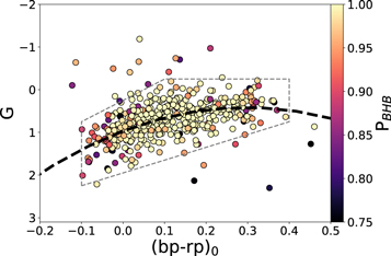
Figure 1. The absolute magnitude of BHB-classified stars, calculated from parallax as a function of dereddened Gaia color. The stars in this figure are most likely to be BHBs, based on their spectra (PBHB ≥ 75%), have less than 10% parallax error, and are observed at z > 750 pc. It is likely that they are all BHBs outside of the plane, and as such exhibit full column reddening, and a relation between the intrinsic color and magnitude may be constructed (the dashed line is a quadratic fit to the data inside the polygon, and is drawn by eye). This figure may be compared to Figure 4 in Deason et al. (2011), which shows a similar BHB color–magnitude distribution, with a similar brightness of around 0.6 in SDSS g (our sample of 13,693 BHBs has a mean abs(G) of ∼0.65). 12
Download figure:
Standard image High-resolution image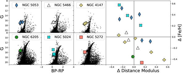
Figure 2. Color–magnitude diagrams of six globular clusters from the Harris (1996) catalog showing BHB stars within 1 tidal radius of their center in our data. The right panel shows the difference between the individual stars [Fe/H] and distance moduli, in relation to the catalog values for their respective clusters. 13 There is an apparent covariance in XGB-predicted G magnitudes and [Fe/H] values, whereby stars which are too metal-poor are predicted to be too bright, and stars which are too metal-rich are predicted to be too dim. The [Fe/H] and G values are predicted by independent machines.
Download figure:
Standard image High-resolution imageWe suggest that the sample of objects used to train our data (having colors b − r < 0.5) may have a different, or negligible, Gaia parallax offset. See, for example, the discussion in Zinn et al. (2019) and their Figures 6 and 7, which shows a parallax-offset trendline in color and temperature, and which may approach zero when considering such hot objects (although the trendline is complex and poorly behaved, and their data do not extend to this color regime).
We have attempted an iterative search of the Gaia parallax offset values, which would produce estimated distance moduli closest to the distance moduli of our globular cluster sample, but the improvement over a zero offset was minor. We feel that such a topic deserves a more thorough investigation than we have given it, but such an investigation would distract from the main thrust of this current work. We simply say that, for our specific sample, it seems unnecessary, and perhaps counterproductive, to include the Gaia parallax zero-point offset. We do, however, encourage anyone using the absolute magnitudes presented in our catalog to investigate this for themselves. The resulting magnitude offset of about 0.3 magnitudes in our sample could produce distance offsets of more than a kpc, and the reader may be better served by assuming a constant or color-dependent absolute magnitude of their own choosing.
We have rerun the entire procedure of this paper with the assumption of a 0.054 mas parallax offset folded in, and the findings are largely unchanged (for example, the high-metallicity BHB sample’s anisotropy changes to 0.73 from 0.70, and our low-metallicity sample’s anisotropy changes to 0.63 from 0.62). The only major difference is that the velocity dispersions in each component drop by about 15 km s−1. This is sensible, as increasing the parallax will raise the estimated absolute magnitudes, and therefore lower the estimated distances to the stars in our sample. The proper motions will then imply lesser tangential motions, leading to lower velocity dispersions.
2.5.1. Optimizing the Machine and Reported Errors
The performance of the machine can be optimized by changing meta-parameters such as the learning rate, the maximal tree depth, etc. To find the optimal parameters, we may split our training data into a training set and a validation set. The machine learns from the training set (75% of the data in each of the three machines), and its performance with various meta-parameters is then analyzed on the validation set (25% of the data; this split simulates the machine’s performance with new, unseen data, by hiding a portion of the data from the machine while it learns, to minimize “data leakage″). We then cycle through various “splits” of the training data. This is a technique known as “cross-validation.” We perform a random grid search of meta-parameters to minimize the mean-squared error (for metallicity and absolute magnitude), or to maximize precision (purity, i.e., minimizing the number of false-positive contaminants, not maximizing the number of true positives) for the classification problem.
After this optimization of meta-parameters, we use the entire training set to train the XGB machine, before predicting values for the complete observational dataset.
The machine self-reports a classification purity (precision) of 85.8% for BHB stars, 14.2% contamination, and successfully finds (recalls) 86.2% of all the BHBs for which there are spectra. We have constructed a confusion matrix based on the results of 100 train–test splits of our training data in Table 2.
Table 2. The Confusion Matrix for Our XGB Classification
| Precision | Recall | |
|---|---|---|
| BHB | 85.8% | 86.2% |
| Not BHB | 90.0% | 89.8% |
Note. Precision (also known as purity) indicates the number of true positives as a percentage of all positive classifications. So 85.8% of all objects classified as a “BHB” are true BHBs. Recall (also referred to as completeness) indicates the fraction of objects which are correctly classified. Briefly, 86.2% of all BHBs in our data are classified as BHBs. This table is based on 100 training–testing splits of the data.
Download table as: ASCIITypeset image
The metallicities are estimated based on a mean-squared error of ∼0.15 dex, or σ[Fe/H] ∼ 0.39 dex. We investigate the metallicity precision as a function of metallicity in Table 3 by again performing 100 train–test splits of our data. We find that the metallicity error is lower for those bins where training data is abundant, from −2.5 ≤ [Fe/H] ≤ −1.5, and less precise where training data is sparse.
Table 3. The Precision of the Metallicity Estimate as a Function of Metallicity
| [Fe/H] | N | σ[Fe/H] |
|---|---|---|
| −3.0 to −2.5 | 43 | 0.77 |
| −2.5 to −2.0 | 169 | 0.31 |
| −2.0 to −1.5 | 232 | 0.23 |
| −1.5 to −1.0 | 83 | 0.45 |
| −1.0 to −0.5 | 24 | 0.82 |
Note. To construct this, we trained the XGB machine with 100 training–testing splits of the total training data, and evaluated the precision of the metallicity estimate of the machine based on those splits. The precision seems to worsen for the highest- and lowest-metallicity BHBs, perhaps because of the lower number of objects in those training sets. One BHB from the training set is missing from this table; it has a metallicity of −0.31.
Download table as: ASCIITypeset image
We note that our training data are extremely sparse with respect to high metallicities. Only 25 have metallicities ≥ −1 dex. This will cause difficulty for the machine when it comes to predicting metallicities higher than −1 dex.
Absolute magnitudes have precisions around σG ∼ 0.41, and show no coherent trend with metallicity.
2.6. Verifying the Regressions
Through cross-validation, we have obtained estimates for the mean-squared error of the metallicity and absolute magnitude estimates, as well as purity estimates, for our BHB classification. Here, we attempt to verify these in a few independent ways.
2.6.1. Color–Magnitude Diagram
A simple way to look at contamination would be to construct a color–magnitude diagram of classified BHB stars. A pure sample should follow the horizontal branch, and contamination should appear off of that branch, probably in redder and dimmer regions, where the most numerous contaminants (MSA stars) reside.
In Figure 1 we show the color–magnitude diagram for stars estimated to be BHBs by our classifier. The stars are selected only to have ϖ errors of 10% or less, and also to be outside of the plane (zXGB > 750 pc, so that the color and magnitude values are reliable after extinction correction, assuming the full columns of Schlegel et al. 1998). We believe that this sample should reasonably reflect the full sample in its proportions of BHB and non-BHB stars, with reference to Table 1, and noting that the proportion of BHBs in the 10% parallax error sample is 34%, rather than the 42% figure for the entire sample. This figure shows a strong concentration of presumptive BHBs, with some contamination extending redwards and fainter (presumably, MSA stars, which includes blue stragglers here), and some contamination brighter and blueward (this could be due to quasars, extreme horizontal branch stars, or possibly true BHB stars which have been over-corrected for extinction, moving them to the too-bright and too-blue sections of the diagram). Traditionally, main-sequence A stars are the most prominent contaminants in this type of classification problem.
The selection of height from the plane has been used in place of latitude, in an attempt to improve the accuracy of the dereddening procedure (by guaranteeing that the full column density of the maps of Schlegel et al. (1998) are meaningful for each star) while preserving as many stars as possible. However, despite these efforts, areas of low latitude may still be confused by high extinction values, particularly if the extinction maps have poor angular resolution of the dust near our stars. In the sample detailed above, the lowest latitude BHB candidate is at 8.9°; 97% of the candidates are above a latitude of 15°; 88% are above 20°; and 68% above 30°. There may be some candidates that experience extinction confusion, but the large majority should be in low-extinction directions, and outside of the plane, with reliable colors and magnitudes. Changing our procedure to include a cut such that all stars are more than 30° from the plane does not change the results much; the anisotropy, for example, remains 0.62 for low-metallicity BHBs, and increases to 0.74 from 0.70 for high-metallicity BHBs.
These stars are generally found in the apparent G magnitude range of 10 to 14, with the median near 12.8. Our biggest fear is that some of these objects have been corrected for the full column density extinction of Schlegel et al. (1998), but in fact experience a different level of extinction. Since these reddening maps are calculated based on extragalactic sources, we expect that the reddening values may over-correct (under-correction should not be a problem), shifting the objects to too-blue and too-bright in this figure (Figure 1) with respect to the extinction-corrected colors and magnitudes. We would expect this type of error to manifest as a diagonal cloud, with a negative slope in the figure, as main-sequence stars (which should truly be in the bottom-right corner) are dragged toward the center, and BHB stars (which should truly be in the center) are dragged toward the top-left corner. While some of this may be occurring, such a pattern is not prominent or noticeable in this data subset. There also appears to be no dependence on galactic latitude, supporting our choice of using distance from the plane as a selector.
Note that Figure 1 has heavier contamination when we include stars closer to the plane, and of lower probability of being a BHB star than in our shown plot, which has cuts at 750 pc and 75%, respectively. Including lower-probability stars increases contamination in the dimmer and redder direction, probably due to MSA stars. Including stars closer to the plane populates a plume of high probability BHB “contaminants,” which are bluer and brighter than the BHB locus. This could be true BHB stars which have been extinction-corrected more than they are intrinsically dimmed by dust.
To obtain a rough estimate of the contamination levels, we draw a polygon around what we presume to be “true” BHBs by eye. Here, 23 out of 450, or 5% of the plotted stars, lie outside this polygon. This is lower than the machine-reported 14% contamination, although there may also be contamination inside of this selection box. If we construct the same figure with cuts of 50% PBHB and z > 500 pc, this changes to 10% lying outside of the polygon. This color–magnitude diagram is indicative of our data in this current work, but not for the entire catalog. The interested party is encouraged to take note of this. We discuss the contamination profile inside the plane more thoroughly in a companion paper.
2.6.2. Globular Clusters
Globular clusters have well-defined distances and metallicities in the literature. By cross-matching our data on the sky to within one tidal radius of the globular clusters in the Harris Catalog (Harris 1996; 2010 revision), we find 20 stars classified as BHBs in six clusters. We show the distance modulus and abundance values of these six clusters and 20 stars in Table 4, and plot them in Figure 2.
Table 4. BHBs Residing within One Tidal Radius of the Globular Clusters Shown in Figure 2
| Globular | Glob. [Fe/H] | BHB [Fe/H] | Glob D. Mod. | BHB D. Mod. |
|---|---|---|---|---|
| NGC 6205 | −1.53 | −1.89 | 14.26 | 14.24 |
| NGC 5466 | −1.98 | −2.03 | 16.02 | 15.92 |
| −2.18 | 16.09 | |||
| −1.9 | 15.88 | |||
| NGC 5272 | −1.5 | −1.96 | 15.04 | 15.18 |
| NGC 5053 | −2.27 | −1.75 | 16.2 | 15.99 |
| −1.95 | 15.94 | |||
| −1.92 | 16.16 | |||
| −2.35 | 16.49 | |||
| −2.33 | 16.34 | |||
| −1.86 | 16.3 | |||
| NGC 5024 | −2.1 | −1.96* | 16.26 | 14.27* |
| −1.89 | 16.38 | |||
| −1.71 | 16.15 | |||
| −1.52 | 16.0 | |||
| NGC 4147 | −1.8 | −1.77 | 16.43 | 16.15 |
| −2.21 | 16.97 | |||
| −1.89 | 16.26 | |||
| −2.07 | 16.73 | |||
| −1.82 | 16.45 |
Note. The asterisks indicate an item omitted from the right panel of Figure 2 because its distance modulus is a large outlier (∼2 mag).
Download table as: ASCIITypeset image
With regard to the apparent visual outlier in NGC 5024, we find that the three stars lying visually on the horizontal branch have proper motions of (μR.A., μDec.) = (−0.09, −1.64), (−0.25, −1.9), and (−0.14, −1.26), and that the outlier has a proper motion of (−0.31, −1.42). This proper motion seems consistent with cluster membership (as does the radial velocity). It could possibly be a true BHB member of the cluster with a highly uncertain photometric magnitude, although that seems unlikely, as its flux error is well below 1%. It is also not likely to be an RR Lyrae (which would be located in a similar place on the color–magnitude diagram), as it is observed two magnitudes from the horizontal branch, whereas RR Lyrae typically only have pulsations on the order of one magnitude. This star is removed from the subsequent analysis of [Fe/H] and abs(G) errors, although we note that its inclusion actually improves the expected precision of the [Fe/H] calculation.
We compare the estimated [Fe/H] values of the member BHBs from the XGB regression with the literature values of their clusters’ metallicities from the Harris Catalog. The error (assuming that the catalog values are exact and true) for our 19 stars (20, minus one visual outlier) is σ[Fe/H] ∼ 0.31. This is slightly more precise than the machine estimated value of σ[Fe/H] ∼ 0.39. Perhaps this is because the metallicities of these globular clusters lie between −2.5 and −1.5, where we predict the [Fe/H] errors to be lower (see Table 3).
For each star in these globular clusters, we may also assign a distance modulus value,

which can be compared to the distance moduli of the globular clusters, modG.C..
If we assume that the error on the observed magnitude, g0, and the distance modulus of the globular cluster, modG.C., are small compared to the error on GXGB, then:

12 This value of σG ∼ 0.21 is substantially lower than the error of σG ∼ 0.41 estimated by the machine. When the outlier discussed previously is included, σG ∼ 0.48. While we do not have a definitive reason as to why, it could be that the data we used for training the absolute magnitudes has some MSA or blue straggler star contamination, which increases the magnitude estimate spread, while the globular cluster fields, being old populations, are deficient in this contamination.
Note that the purity of this sample is about 95% (if the star lying off the horizontal branch, in NGC 5024 is in fact a contaminant, and not a field BHB). This is similar to the machine-reported contamination values, but should not be given too much weight, as these observational fields should naturally be overabundant in BHBs.
In Figure 2 we note that there seems to be a slight covariance between the distance modulus offset and the metallicity offset. To try and correct for this, we attempt a multi-output regression, i.e., fitting the metallicity and the absolute magnitude simultaneously. Unfortunately, the Century Survey and the Xue et al. (2008) sample combined only contain nine BHBs with metallicities and good parallax measurements which lie outside the plane (having good G measurements). These nine objects also only span −2.0 ≤ [Fe/H] ≤ −1.5, which would exacerbate our noted problems with predicting high-metallicity values for our data. We abandon this line of inquiry, and accept the covariance.
This covariance could be an effect of how temperature and metallicity affect spectral line shape. Larger brightnesses tend to characterize lower surface gravity stars, which have narrower spectral lines. Larger abundances tend to make lines deeper. A deep, wide line (high abundance, low brightness) could have a similar overall shape to a shallow, narrow line (low abundance, high brightness) on a normalized spectra. Confusion between these two could cause the machines to mistakenly lower the abundance of a given spectrum while also increasing the brightness, leading to the covariance we see.
This could possibly be avoided with higher resolution spectra, as these two effects actually affect the line shape in subtly different ways, particularly in relation to the wings of the profile.
2.6.3. Duplicates
The LAMOST survey has observed numerous stars over multiple observations; some of these duplicate observations have been classified by the XGB machine as BHB stars. Since the spectra are independent of each other, they provide some insight into internal errors in classification and regression. In Figure 3 we show the distribution of magnitudes and metallicities for stars observed two or more times. Based on this Figure, we see that the median σ[Fe/H] is about 0.07, and the median σ G is about 0.06. 14
Note that duplicates are removed in the analysis section of the paper (preserving the observation with the highest signal-to-noise ratio), but are not removed from the catalog.
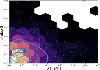
Figure 3. σ[Fe/H] and σG values for stars (blue points and hex map) observed two or more times (under different observation conditions) by LAMOST. The contours indicate the smoothed 25%, 50%, and 75% confidence intervals, and the cross indicates the median σ[Fe/H] and σG (0.07 and 0.06, respectively).
Download figure:
Standard image High-resolution imageIn our sample of 13,693 BHB spectra, we estimate that there are 11,046 unique stars. There are 1884 objects for which there are multiple observations; the largest number of repeated observations is one star with 16 individual spectra, and the median is two observations per star.
3. Coordinates and Velocities
Kinematic phase information is calculated in the usual way, on the basis of observed coordinates, proper motions, radial velocities, and the distances derived from the XGB-predicted absolute magnitudes, and photometry which has been extinction-corrected using the full column dust maps of Schlegel et al. (1998). 15
Our coordinates are all right-handed, with the Sun at (X, Y, Z) = (−8.27, 0, 0), rotating with a velocity of (VR , Vϕ , VZ ) = (0, −236, 0) km s−1; VR is positive away from the Galactic center. The solar motion is (U, V, W) = (13.0, 12.24, 7.24) km s−1 with respect to the local standard of rest. These positions and velocities are all adopted from Schönrich & Aumer (2017), and Schönrich (2012).
The final assignment of these coordinates is based on the mean value of 100 realizations of the observed star, considering the observational errors as well as the Gaia correlations for the relevant parameters.
3.1. Final Cuts for Halo BHBs
Coverage of our sample is shown in Figure 4. The catalog covers a large area of sky, unexplored by prior BHB surveys. However, for the rest of this paper, we will only consider stars which are observed at more than 3 kpc from the plane, from which we select halo BHBs. In a companion paper, we will conduct a more thorough analysis of the BHB population closer to, and inside of, the plane.
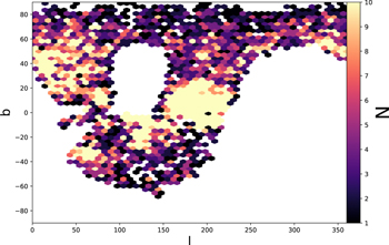
Figure 4. Sky coverage of our BHB sample. It can be seen that our BHB sample covers a good amount of the plane which is not covered in other large BHB catalogs. Note that this is the full catalog; the subset analyzed below is restricted to stars more than 3 kpc away from the plane.
Download figure:
Standard image High-resolution imageFrom our initial Gaia–LAMOST crossmatch of 155,549 objects, 14,101 are classified as BHBs. We remove objects for which the machine has predicted values outside of the input parameter range for G (from −2.5 to −1.2) and [Fe/H] (from −3 to −0.3), from the catalog, leaving a total of 13,693 BHBs in our final catalog.
We make the following additional cuts to the catalog, so as to prepare the scientific sample for the remainder of this paper: duplicates removed within 7″, e μR.A., e μdecl. < 10%, e(r.v.) < 10%, PBHB > 75%, z > 3 kpc, 3 σ velocity outliers iteratively culled.
This leaves 2692 high-confidence BHBs in our halo sample with good kinematics; these constitute the data for the rest of the analysis in this paper.
4. Analysis
4.1. Anisotropy
Anisotropy is an observable measurement of the degree to which a population is orbiting tangentially versus radially in the galaxy:

Populations which are radially biased have β > 0, and tangentially-biased populations have β < 0.
In Figure 5 we plot the velocity dispersions and anisotropy of our sample in high- and low-metallicity subsets as a function of spherical radius. We find that the halo sample has relatively flat anisotropy for both high- and low-metallicity bins, with the low-metallicity stars being more tangential velocity dispersion-dominated (β ∼ 0.62), and the high-metallicity stars being more radial velocity dispersion-dominated (β ∼ 0.70). We note that the radial velocity dispersion is similar between the two populations, whereas the tangential velocity dispersion of the metal-rich stars is lower than that of the metal-poor stars.
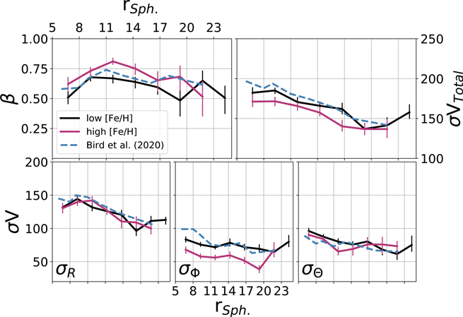
Figure 5. Top left: anisotropy is a measure of how radial the orbits of a population are. The metal-rich stars in our sample are slightly more radial than our metal-poor stars. Top right: total velocity dispersion of the BHB sample falls within a spherical radius, with metal-rich BHBs usually being cooler than metal-poor BHBs. Bottom: individual components of the velocity dispersions, used to derive the upper panels. The panels include the findings of Bird et al. (2020) for their “all SDSS halo BHB” sample, and the agreement seems good. We refer the reader to that paper for a more detailed analysis of their BHB and K-giant data, including metallicity dependence, and a more thorough removal of substructure than we have implemented here. We have used the “extreme deconvolution” method of Bovy et al. (2011) to calculate the velocity dispersions.
Download figure:
Standard image High-resolution imageBird et al. (2019) analyzed the anisotropy parameter using LAMOST K-giants, which are a younger population than BHB stars. They found a generally more radial population, with β ∼ 0.8 at Galactocentric radii less than 20 kpc, which becomes more tangential at larger radii, before reaching an almost isothermal value of zero at 100 kpc. Interestingly, they also split their population based on metallicity (their Figure 5) and found that their lowest-metallicity K-giants have β ∼ 0.6, while higher-metallicity K-giants are closer to β ∼ 0.8. This metallicity trend of larger β values for metal-rich stars is consistent with our results, although our population of BHB stars seems to be generally more tangential velocity dispersion-dominated than their population of K-giants.
Wegg et al. (2019) recently looked at the anisotropy and velocity ellipsoids of RR Lyrae stars, out to a spherical Galactocentric radius of about 20 kpc. Their sample is similar in both age and extent to our current BHB population. They found that the velocity profiles of RR Lyrae become highly radial beyond 5 kpc, with β ∼ 0.8; inside that radius, they are more tangential, with a prograde rotation 16 of about 50 km s−1, and with β down to 0.25. Our sample is less radial velocity dispersion-dominated than their sample, and does not probe as low in the galactocentric radii as theirs does. It is worth noting that their study probed latitudes down to 10°, which would bring their observational window closer to the disk than the window considered in this work.
Analyses of cosmological simulations generally find that the β parameter rises with galactic radius. At their centers, simulated galaxies are nearly isotropic. Moving outward, the halos of galaxies tend to become more radially biased, with β rising, at first quickly and then more slowly, to a value ≥0.7 beyond 10 kpc from the center (see Loebman et al. 2018 and discussion therein).
Note that we have not removed substructure in this analysis. Our sample should not suffer from large amounts of major substructure contamination, as our sample does not extend to the distance of major contaminants, such as Sagittarius (our sample cuts off around 20 kpc).
4.2. Ages and Metallicities
Nearly thirty years ago, Preston et al. (1991) noted that BHB stars exhibited a color gradient in the halo, growing redder with increasing radius. They posited that such a color gradient could be the result of an age gradient in the halo, with redder BHB stars being, on average, younger. 17
This work has been revisited recently, with reference to Sloan Digital Sky Survey spectroscopy (Santucci et al. 2015) and photometry (Carollo et al. 2016, see also Whitten et al. 2019). They similarly find a suggestion of a reddening of BHB color with increasing radius, with the bluest (oldest) stars being more centrally concentrated.
We plot the colors, as well as the metallicities of our BHB sample in Figure 6. This Figure shows that as we move outward in the halo, the BHB population grows redder (perhaps younger), and metallicity remains relatively flat, at around −1.9 dex. This abundance value is similar to that expected for the halo, if a little high; Xue et al. (2008) found a value of around −2 dex in their sample.
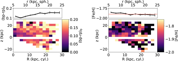
Figure 6. Left: the colors of our BHB stars as a function of distance from the plane, and radius (cylindrical in the bottom frame, spherical in the upper frame). Color may be a proxy for age in BHBs, with redder BHBs coming from younger populations. This figure shows a clear trend for more distant BHB stars to be redder, and therefore to possibly represent a younger population. Right: similar to the left-hand frames, but related to metallicity rather than color.
Download figure:
Standard image High-resolution image5. Discussion
In our halo sample, we have noted two trends:
- 1.Our metal-rich BHB stars move on more radial orbits than our metal-poor stars at all radii.
- 2.As we move outward in the halo, the BHBs grow redder (possibly younger), while metallicity remains relatively flat.
When speaking of the halo, there are a few main paradigms. The first is the idea of an inner and outer halo, two major components which overlap, but which trade dominance as radius increases, leading to a sort of “break” where the outer halo becomes the more dominant population. The inner halo is thought to be slightly prograde and more metal-rich, while the outer halo is thought to be slightly retrograde and more metal-poor. This idea has been pursued vigorously, with mounting evidence provided by the research group of Carollo et al. (2007). This finding has been supplemented with evidence from other teams,revealing broken halo-density profiles in various tracers (e.g.: BHBs Deason et al. 2011 and Deason et al. (2018), RR Lyrae Sesar et al. 2011), in the presence of two major components in the chemistry (Nissen & Schuster 2011, and subsequent papers in that series), in a broken age profile in the halo (Whitten et al. 2019), and in the exotic stellar-population prevalences (Carollo et al. 2012).
A more recent development, revealed primarily via the exquisite proper-motion data from Gaia, is couched in terms of merger history. The discovery papers of Belokurov et al. (2018) and Belokurov et al. (2020) detail two major halo components, dubbed “The Sausage” and “The Splash,” respectively. The Sausage is a highly radial population of stars, thought to have arisen from a merger occurring 8–11 Gyr ago with a 1010 M⊙ galaxy, and the Splash is thought to be debris from the Milky Way’s proto-disk at the time of this merger. The Splash is slightly younger, by perhaps a Gyr, and more metal-rich ([Fe/H] > −0.7, while the Sausage is found to have a metallicity of around [Fe/H] between −1.7 and −0.7). The Splash stars generally have low angular momentum, and some have retrograde orbits (see also Amarante et al. 2020).
The “Gaia Enceladus” theory of Helmi et al. (2018) combines the retrograde halo with the eccentric Sausage into a single event. Other groups (e.g., Myeong et al. 2019) propose that the Sausage arose from a single merger, while the retrograde component arose from a separate event, known as “Sequoia.” Sequoia stars are thought to be slightly more metal-poor than Sausage stars.
Comparing metal-rich to metal-poor components at different radii, we find that our metal-rich BHBs seem to be more radial velocity dispersion-dominated (having higher β), which could imply that they contain a significant portion of “Sausage” members. We briefly inspect the VR − Vϕ velocity plane in Figure 7, finding that a portion of our high-metallicity stars reside in an extended VR feature around zero rotation, which is consistent with the Sausage’s kinematic feature.
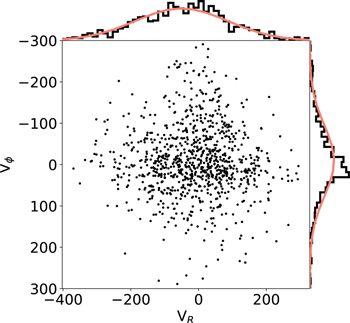
Figure 7. The VR Vϕ plane of our BHBs with metallicities > −1.8 and Z > 3 kpc. It can be seen that our sample is roughly Gaussian in VR , as expected for the canonical halo population. However, the Vϕ distribution is not well-fitted by a Gaussian, having a strong peak near zero, and a heavy tail extending toward prograde rotation. This peak near zero is indicative of the sausage-like feature given in Belokurov et al. (2018), in their Figure 2. The heavy tail extending toward prograde rotation could be related to the thick disk–halo interface.
Download figure:
Standard image High-resolution imageWe briefly check for the presence of the Sequoia/Enceladus feature by investigating our most metal-poor BHBs; however we do not see evidence of these less enriched BHBs having a surplus of counter-rotating members, so we do not think a substantial number of stars exhibiting such features are present in our sample.
At this point, we return to our other finding, i.e., that our BHB stars possibly grow younger with increasing radius, while the metallicity gradient remains flat.
When looking at the globular cluster population of the Milky Way, in situ globular clusters generally populate an area of around 12-14 Gyr in age, with metallicities mainly being between −0.5 and −1.5, and a slight tail extending to lower metallicities. Accreted globular clusters follow a track which moves from age = 14 Gyr and [Fe/H] = −2.5 dex to age = 10 Gyr and [Fe/H] = −1.25 dex (i.e., a track which is more metal-poor for a given age, or younger at a given metallicity, than the in situ clusters, see Forbes 2020). 18
It has also been suggested via simulations that minor mergers, with masses in the range of 1:50 or 1:100 that of the Milky Way, are expected to deposit more debris in the outer regions of the Galaxy, as compared to major mergers (Karademir et al. 2019).
In Λ CDM simulations of Milky Way type galaxies, it is often found that mass buildup is dominated by early accretions (Bullock & Johnston 2005). Since these early accretions are generally larger, they experience more dynamical friction, and sink toward the center; this leads to the oldest stars being most commonly found in the very central portions of the galaxy (Tumlinson 2010). If there are several accretions, these can flatten the halo metallicity gradient, and if there are few, then a steeper gradient is expected (Cooper et al. 2010).
It is also expected that systems in more quiescent regions may continue their star formation longer than those which are quenched due to merging processes and chaotic environments (Balogh et al. 1999). As such, smaller accretions at later times could possibly host younger populations.
In our data, we see a relatively flat metallicity gradient, which would imply that the Milky Way has experienced several mergers, rather than a few. We also see a color gradient, which could be interpreted as an age gradient, with younger stars in the external regions. We suspect that these younger, peripheral stars come from minor mergers with smaller satellite systems (shifting them to the external regions of the halo), which have less intense star formation owing to their lower masses (shifting them to lower metallicities for a given age), and have been accreted at later times than the older halo stars from earlier major mergers (allowing their star formation to continue longer outside of the quenching effects of accretion, and thus host younger stars).
In short, we see evidence in the anisotropy parameter for a portion of our data to be associated with the Gaia Sausage event (having a higher β, and therefore being more radial). We do not find indications of our data belonging to the Splash or Sequoia/Enceladus, as we see no retrograde component beyond what is expected from the canonical halo at low metallicities. We suggest that we see evidence for the outer regions of our footprint predominantly comprising accreted stars from smaller accretion events at later epochs.
6. Conclusions
We have implemented a machine-learning algorithm to classify LAMOST spectra with blue Gaia colors as either BHB or not-BHB objects. This classification is approximately 86% pure. Please note when using this catalog that this is more complicated for lower machine-probability stars, and stars closer to the plane, although even in the worst case, the catalog should be at least ∼60% pure. We will discuss this in more detail in our companion paper. We similarly (with a second machine) predict metallicities to about 0.35 dex, although we note that our sample does not contain many [Fe/H] values above −1 dex. This is probably a limitation of our training data, and it is better to consider the derived metallicities as relative values, rather than absolute values. We predict absolute magnitudes to ∼0.31 mag using a third machine, which is trained using parallax distances. We verify the classification and regressions via the investigation of color–magnitude diagrams of both sample and globular cluster comparisons. In this comparison, we note that there is covariance between the estimated metallicity and absolute magnitude, with those stars estimated as too bright also being too metal-poor. However, despite this, a comparison with globular clusters yields errors near to 0.3 dex in [Fe/H] and 0.2 in magnitude, with no significant systemic offset from cluster values found in the literature.
This catalog comprises the largest database of BHB stars thought to currently exist within the extent of the disk. Other large spectroscopic catalogs, notably those from the SDSS, largely avoid the plane latitudes, and have higher apparent magnitude limits, which forces their BHB observational windows out of the disk regions. Color-based selection of BHBs inside the plane is difficult, given that color is reddening-dependent, 19 and reddening is largely unknown inside the plane, with the exception of three-dimensional reddening maps, which remain difficult to construct precisely. 20 Outside the plane, extinction may be regarded as a known quantity, thanks to the invaluable maps of Schlegel et al. (1998). Spectroscopic identification, as performed here, does not suffer from this extinction confusion, however. This catalog therefore presents interesting and novel opportunities to study this species of star in a hitherto unexamined regime.
We have briefly investigated the halo properties of our BHB stars. We find that our metal-rich BHBs are on more radial orbits at all galactocentric radii. We interpret this as indicating that the metal-rich population in our sample is populated by Gaia Sausage stars, in addition to halo stars, whereas the metal-poor stars do not obviously belong to any of the other named major merger components.
We find that as we move outward in the halo, from about 5–20 kpc, the BHBs grow redder (which could mean younger) and that the metallicity gradient remains mostly flat.
If we suppose that the inner region is populated mostly by large accretion events, and the outer region by smaller ones, then we would expect a decreasing metallicity gradient and a flat age gradient, if the mergers occurred at the same time, and star formation in the systems was subsequently quenched simultaneously (since larger systems have higher star formation rates, and should intuitively be more enriched).
If, instead, the larger, centrally concentrated accretions occurred prior to the smaller accretions, their star formation would be quenched at earlier epochs, and as such, we would perhaps see a decreasing age gradient in the stellar populations as we move outward in the halo to the areas populated by smaller, more recent mergers. In this situation, we may not expect a decreasing metallicity gradient with radius; if the outer regions are quenched at later epochs, they may have had more time to enrich, and their abundance levels may “catch up” with those of the larger systems at the center.
In this paper, we have investigated only BHB stars in our catalog which reside far from the plane, in the halo, omitting more than half of our data. Dealing with the data in the plane requires a more nuanced and rigorous investigation of the effects of differential reddening (given that our distances here are photometrically derived), and larger contaminating populations. A second paper has been prepared, which \deals specifically with the data from inside the plane. The catalog may be downloaded from https://zenodo.org/record/4547803.
We thank the referee for their thoughtful comments, which helped improve the clarity of this paper.
We thank Corrado Boeche for his work in normalizing the LAMOST spectra so that we could easily utilize them in this work.
We thank Iulia Simion for helpful discussions and suggestions regarding Gaia kinematics.
We thank the developers and maintainers of the following software libraries used in this work: Topcat (Taylor 2005), NumPy (van der Walt et al. 2011), SciPy (Virtanen et al. 2020), AstroPy (Astropy Collaboration et al. 2013), matplotlib (Hunter 2007), scikit-learn (Pedregosa 2011), IPython (Perez & Granger 2007), XGBoost (Chen & Guestrin 2016) and Python.
The research presented here is partially supported by the National Key RD Program of China, under grant No. 2018YFA0404501, by the National Natural Science Foundation of China under grant Nos. 12025302, 11773052, and 11761131016, and by the “111” Project of the Ministry of Education under grant No. B20019. This work made use of the Gravity Supercomputer at the Department of Astronomy, Shanghai Jiao Tong University, and the facilities of the Center for High-Performance Computing at Shanghai Astronomical Observatory.
J.J.V. gratefully acknowledges the support of the Chinese Academy of Sciences President’s International Fellowship Initiative. M.C.S. acknowledges financial support from the CAS One Hundred Talent Fund, and from NSFC grants 11673083 and 11333003.
Guoshoujing Telescope (the Large Sky Area Multi-Object Fiber Spectroscopic Telescope LAMOST) is a National Major Scientific Project, built by the Chinese Academy of Sciences. Funding for the project has been provided by the National Development and Reform Commission. LAMOST is operated and managed by the National Astronomical Observatories, Chinese Academy of Sciences.
This work has made use of data from the European Space Agency (ESA) mission, Gaia (https://www.cosmos.esa.int/gaia), processed by the Gaia Data Processing and Analysis Consortium (DPAC, https://www.cosmos.esa.int/web/gaia/dpac/consortium). Funding for the DPAC has been provided by national institutions, in particular the institutions participating in the Gaia Multilateral Agreement.
Footnotes
- 4
“Purity,” also referred to as “precision,” refers to the number of true positives, based on all positive classifications. “Contamination” refers to the number false-positive misclassifications, based on all positive classifications (one minus the purity). “Completeness,” also known as “recall,” refers to the number of “true positive” classifications, based on all true positives (i.e., the proportion of true candidates which are successfully recovered).
- 5
For the purposes of this paper, a blue straggler star will be considered as an MSA star, as they are similar in terms of observational qualities.
- 6
Sometimes the profile is fit with a Voigt profile, which is a combination of a Gaussian core and Lorentz wings, representative of the differing effects on spectral line shape of abundance and gravity.
- 7
In most cases, some techniques, such as those based on decision trees, construct a series of yes-no questions.
- 8
Large redshifts artificially compress our rest spectra to be smaller than the grid we use. This cut probably removes spectra of blue items at large distances, such as quasars.
- 9
- 10
A problem common to decision trees, and a risk inherent in all supervised machine-learning techniques, is so-called “overtraining,” whereby the machine memorizes the training data exactly. This provides excellent precision and recall of the training data, but poor metrics for unseen testing data. This is why the individual components must be kept “weak”; however, the resulting conglomerate will be “strong.”
- 11
The 41 BHBs with missing metallicity values all occur in the catalog of Xue et al. (2008). In their work, they classified BHB stars based on a line-shape method which they implemented themselves on the SDSS spectra, and the reported metallicities were collected using a separate calculation, the WBG pipeline in SDSS. The WBG, or “Wilhelm, Beers, and Gray” pipeline, is optimized for the treatment of hot stars, such as BHBs, and the details may be found in Wilhelm et al. (1999). It is unclear why the SDSS pipeline was unable to assign a metallicity to these stars, while Xue et al. (2008) were able to calculate their line parameters for classification purposes. We note that the stars with missing values seem to be preferentially bluer and dimmer than the bulk of the sample in Xue et al. (2008).
- 12
The obvious visual outlier in NGC 5024 is omitted from the right-hand panel, as its distance modulus is an extreme outlier. The star is presented in Table 4.
- 13
Including lower-probability BHB stars (PBHB between 0.5 and 0.75) increases main-sequence contamination to the red and dim corner of the plot. Including lower z-height data creates a plume of contamination along the reddening vector to the brighter, bluer corner, which could be ascribed to true BHBs, incorrectly dereddened. This figure should be simple to reproduce with the provided catalog crossmatched to Gaia, so the interested reader is encouraged to examine how these effects change, depending on your own cuts.
- 14
These values are much smaller than the dispersions discussed previously, i.e., 100 spectra of stars with similar metallicity or brightness would have a larger spread in [Fe/H] and abs(G) than 100 spectra of the same star. This may imply that the fitting surface is not smoothly varying, which is a side-effect of random forest algorithms, or that some third parameter, such as surface gravity, or temperature, works to inflate the errors.
- 15
We use full column reddening here, as we will later cut the data to have a distance of more than 3 kpc from the plane, in order to select halo stars. When using these data at lower altitudes, a different procedure is necessary.
- 16
Our sample is slightly retrograde in the area studied (z > 3 kpc), near −20 km s−1.
- 17
They noted that the color gradient could also be the result of more distant BHB stars having smaller core masses, but found no reasonable explanation as to why that may be the case; see also the “second parameter phenomenon” of BHB morphology, explored in detail in Dotter et al. (2010).
- 18
The Sagittarius-associated globular clusters, for example, have ages up to four Gyr younger than the in situ Milky Way clusters at similar enrichment levels, and the Sagittarius stream is prominent at distances up to 80 kpc in the halo. Alternatively, the Gaia Enceladus-associated globular clusters have metallicities 1 dex lower than in situ globular clusters at similar ages.
- 19
Particularly ultraviolet wavelengths, such as the U band, which is frequently used for BHB identification.
- 20