Abstract
Polarization of starlight and thermal dust emission caused by aligned dust grains is a valuable tool to characterize magnetic fields (B-fields) and constrain dust properties. However, the grain alignment physics is not fully understood. To test the radiative torque (RAT) paradigm, including RAT alignment (RAT-A) and disruption (RAT-D), we use dust polarization observed by Planck and Stratosphere Observatory for Infrared Astronomy/High-resolution Airborne Wideband Camera Plus toward two filaments, Musca and OMC-1, with contrasting physical conditions. Musca, a quiescent filament, is ideal for testing RAT-A, while OMC-1, an active star-forming region OMC-1, is most suitable for testing RAT-D. We found that polarization fraction, P, decreases with increasing polarization angle dispersion function,  , and increasing column density, N(H2), consistent with RAT-A. However, P increases with increasing dust temperature, Td, but decreases when Td reaches a certain high value. We compute the polarization fraction for the ideal models with B-fields in the plane of sky based on the RAT paradigm, accounting for the depolarization effect by B-field tangling. We then compare the realistic polarization model with observations. For Musca with well-ordered B-fields, our numerical model successfully reproduces the decline of P toward the filament spine (aka polarization hole), having higher N(H2) and lower Td, indicating the loss of grain alignment efficiency due to RAT-A. For OMC-1, with stronger B-field variations and higher temperatures, our model can reproduce the observed P–Td and P−N(H2) relations only if the B-field tangling and RAT-D effect are incorporated. Our results provide more robust observational evidence for the RAT paradigm, particularly the recently discovered RAT-D.
Original content from this work may be used under the terms of the Creative Commons Attribution 4.0 licence. Any further distribution of this work must maintain attribution to the author(s) and the title of the work, journal citation and DOI.
1. Introduction
Dust is a crucial element of the interstellar medium (ISM) and has a significant impact on a variety of astrophysical processes, such as gas heating and cooling, the formation of stars and planets, and surface astrochemistry (see Draine 2003 for an overview). Moreover, the polarization of starlight (Hall 1949; Hiltner 1949) or polarized thermal dust emission (Hildebrand 1988) induced by aligned dust grains are widely used to observe magnetic fields (B-fields), which are predicted to regulate the formation and evolution of molecular clouds and filaments, star formation, and stellar feedback via outflows/jets (see Crutcher 2012; Pattle & Fissel 2019; Pattle et al. 2023 for reviews). Thermal dust polarization has also been used to map B-fields in nearby galaxies (e.g., Lopez-Rodriguez et al. 2022) and even in high-z galaxies (Geach et al. 2023). Moreover, dust polarization is a valuable tool to probe dust physics and dust properties (size, shape, and composition, see, e.g., Draine & Hensley 2021).
Dust polarimetry is based on the assumption that dust grains are systematically aligned with the ambient B-fields with their longest axes perpendicular to the fields. Hence, the polarization vectors of thermal dust emission are perpendicular to the B-fields projected on the plane of the sky (POS). Therefore, by rotating the observed polarization angle by 90°, we can infer the morphology of the B-fields (e.g., Hildebrand 1988).
To establish dust polarimetry as a reliable diagnostic tool to probe B-fields and dust properties, it is necessary to fully understand the detailed physics of grain alignment. The leading mechanism of grain alignment is based on the radiative torques (RATs), arising from the differential scattering and extinction of an anisotropic radiation field by nonspherical grains (Dolginov & Mitrofanov 1976; Draine & Weingartner 1997; Lazarian & Hoang 2007). The key prediction of the radiative torque alignment (RAT-A) theory is that the degree of grain alignment depends on the local conditions, including the gas density and radiation, such that the alignment degree decreases with increasing the local density mainly due to gas randomization but increases with the radiation field intensity or dust temperature due to the more efficient alignment of grains in stronger radiation fields (Hoang & Lazarian 2014; Lazarian & Hoang 2019). As a result, the RAT-A theory predicts two key features, including (1) the anticorrelation of the polarization degree, P, with the gas density, and (2) a correlation between P and the intensity of the radiation field (or dust temperature; see Hoang et al. 2021).
Previous tests of RAT-A using starlight polarization support the key predictions of the RAT theory (see Andersson et al. 2015). For instance, observations toward different regions usually report the general trend of the decrease in the polarization fraction with the gas column density, which is known as the polarization hole, by both optical−near-IR (e.g., Whittet et al. 2008) and far-IR/submillimeter polarization observations (Ward-Thompson et al. 2000). Numerical modeling by Whittet et al. (2008) and Hoang et al. (2021) showed that the polarization hole could be explained by the loss of grain alignment toward high-density and low radiation field regions based on the RAT-A theory. For a comprehensive review of the successful tests for the RAT-A theory using starlight polarization, please refer to a review by Andersson et al. (2015).
Nevertheless, to date, there is still a lack of comprehensive testing of the RAT-A mechanism using thermal dust polarization. Specifically, there is an ongoing debate regarding the exact cause of the polarization hole observed in far-IR/submillimeter toward molecular clouds and star-forming regions. For the diffuse and translucent clouds, it is found that the B-field fluctuations are likely the main cause of the polarization hole, instead of grain alignment loss predicted by the RAT-A, as found from both observations (e.g., Planck Collaboration XIX 2015) and numerical simulations (e.g., Seifried et al. 2019). Furthermore, the inclination angle of the B-fields with respect to the line of sight (LOS) significantly affects the polarization fraction due to the projection effect (Hoang & Truong 2024). In particular, observations revealed that P does not always increase with Td (Planck Collaboration XII 2020), which is opposite to the key prediction of the RAT-A theory.
Hoang et al. (2019) proposed a new mechanism called radiative torque disruption (RAT-D), which is expected to resolve the later puzzle. The basics of the RAT-D mechanism is that large grains illuminated by an intense radiation field are spun up to suprathermal rotation by RATs, the same driver of grain alignment. When the centrifugal stress induced by grain rotation exceeds the grain's tensile strength, large grains will be disrupted into smaller ones. Numerical modeling of thermal dust polarization by Lee et al. (2020) using a simplified (DustPOL-py) code based on the RAT-A and RAT-D mechanisms (the so-called RAT paradigm) showed that the depletion of large grains by RAT-D causes a decrease in the polarization fraction at long wavelengths when the dust temperature is sufficiently large, which successfully reproduces the anticorrelation seen by Planck. The basic idea of this effect is the following. For a fixed maximum grain size ( ), a higher radiation strength or dust temperature can align smaller grains, broadening the grain size distribution aligned and increasing the thermal dust polarization fraction. However, when RAT-D happens, large grains are disrupted, removing grains from
  to the disruption size (adisr), which results in a narrower grain size distribution and decreases the polarization fraction (see Figure 7 in Tram & Hoang 2022 for a detail). To test the RAT paradigm, previous studies (Ngoc et al. 2021; Tram et al. 2021a, 2021c; Hoang et al. 2022) analyzed far-IR and submillimeter polarization data observed toward star-forming regions by the High-resolution Airborne Wideband Camera Plus (HAWC+) instrument (Harper et al. 2018) on board the Stratosphere Observatory for Infrared Astronomy (SOFIA) and James Clerk Maxwell Telescope (JCMT). They found that P tends to increase with Td but then decreases when Td exceeds some high temperatures, supporting the RAT paradigm. Later, detailed numerical modeling by Tram et al. (2021a, 2021c) using the DustPOL-py code successfully reproduced the P–Td trend observed in the OMC-1 and ρ Ophiuchus A molecular clouds, which showed the initial success of the joint effect of RAT-A and RAT-D.
However, the effects of the B-field fluctuations on the polarization hole and the variation of P–Td have not been considered yet in the previous tests of the RAT paradigm using polarization data (see Tram & Hoang 2022 for a review). It is, therefore, necessary to take into account the effects of B-field fluctuations to achieve a complete testing of the RAT paradigm.
Filaments are ubiquitous and form a complex network within most interstellar clouds, as revealed by Herschel. Filaments are considered the earliest stage of the star formation process in which the gas density and dust temperature vary significantly across the filaments (e.g., André et al. 2014), which makes them ideal targets for testing the RAT paradigm. Therefore, the two main objectives of our study are to (1) test the RAT paradigm and (2) study the effect of the B-field fluctuations on the net thermal dust polarization of aligned dust in filaments. To achieve these objectives, we use dust polarization data observed toward Musca by Planck and OMC-1 by SOFIA/HAWC+ and perform synthetic modeling of the dust polarization with our DustPOL-py code. Our selection of these filaments is intended to account for the different local properties, e.g., the gas density and radiation field (with or without embedded protostars). While Musca is one of the simplest filaments without embedded protostars, Orion is the closest high-mass star-forming region. With low dust temperatures and small B-field tangling, Musca is a perfect target to test RAT-A. With high dust temperatures, OMC-1 is the ideal target for testing RAT-D. We use our DustPOL-py code to perform pixel-by-pixel polarization modeling of the observed polarization data with the key local physical parameters inferred from observations.
This paper is the second one in our series aimed at characterizing the properties of B-fields and dust in interstellar filaments using dust polarization. Our first paper focuses on the B-fields and dust in a massive filament, G11.11-0.12 (Ngoc et al. 2023). We structure this paper as follows. In Section 2, we describe the observational data on which we work, and our data analysis techniques are described in Section 3. Section 4 recalls the basis of our model and shows the comparison with the observational data. We discuss the results in Section 5, and summarize the main findings in Section 6.
2. Observations
2.1. Polarization Data
We use the thermal dust polarization data observed by Planck and SOFIA/HAWC+ from Musca and OMC-1, respectively. Information on these filaments and their observations is provided in Table 1.
Table 1. Properties of Musca and OMC-1 and Their Observations
| Objects | Distance | Facility | Wavelength | Beam Size | Physical Scale a | Reference |
|---|---|---|---|---|---|---|
| (pc) | (μm) | (pc) | ||||
| Musca | 170 | Planck | 850 |

| 0.24 | Planck Collaboration XII (2020) |
| OMC-1 | 388 | SOFIA | 214 | 18 | 0.03 | Chuss et al. (2019) |
Note.
a The scale of the beam size.Download table as: ASCIITypeset image
For linear polarization, the polarization states are defined by the Stokes parameters I, Q, and U. Because of the presence of noise in Q and U, the polarized emission intensity, PI, is debiased by (Vaillancourt 2006)

where δ Q and δ U are the uncertainties on Q and U, respectively. Assuming that δ Q and δ U are uncorrelated, the uncertainty on PI is (Gordon et al. 2018)

The polarization degree, P, and its uncertainty, δ P, are calculated as

and

where δ I is the uncertainty on I, which is provided together with I from observations.
The polarization angle, θ, and its uncertainty, δ θ, are calculated as follows:


For the Planck data, θ is calculated by  because of the different convention used for the Stokes parameters (Planck Collaboration XII 2020).
The polarization direction of thermal dust emission is perpendicular to the projection of B-fields in the POS; therefore, the B-field orientation angles on the POS are obtained by rotating 90° from the polarization angle θ. Following the IAU convention, the angles of the B-field lines are east of north, ranging from 0° to 180°.
2.2. Polarization Angle Dispersion Function
To quantify the tangling of B-fields at small scales, we compute the polarization angle dispersion function, denoted as  (see Section 3.3 in Planck Collaboration XII 2020). For each pixel at location
x
,
(see Section 3.3 in Planck Collaboration XII 2020). For each pixel at location
x
,  is determined as the rms of the polarization angle difference between the reference pixel
x
and pixel i,
is determined as the rms of the polarization angle difference between the reference pixel
x
and pixel i,  . Pixel i is situated on a circle with
x
as the center and a radius of δ:
. Pixel i is situated on a circle with
x
as the center and a radius of δ:

with N as the number of pixels lying on the circle. For the current study, we calculate  for δ taking a value of one beam size of the observations. Due to noise on the Stokes parameters Q and U,
  is biased. The variance of angle dispersion function,
  , and the debiased
  for a certain pixel
x
are calculated as (see Section 3.5 of Planck Collaboration XII 2020)
for a certain pixel
x
are calculated as (see Section 3.5 of Planck Collaboration XII 2020)
and

Here,  can be positive or negative depending on whether the true value is smaller or larger than the random polarization angle of 52◦ (Serkowski 1962; Alina et al. 2016). The data points with
  are removed. Hereafter, we refer to
  as
as  for convenience.
2.3. Dust Temperature and Column Density Maps
For further studies, we adopt the dust temperature and column density maps of Musca and OMC-1 from previous studies. These maps are obtained by fitting a modified blackbody function to the spectral energy distributions (SED).
Musca. The Planck Collaboration uses data collected by Planck at 850, 550, 350 μm and IRAS at 100 μm to fit with a modified blackbody function to obtain all-sky maps of dust temperature, optical depth, and spectral index (Planck Collaboration XI 2014). The resolution of the resulting maps is  . The dust temperature and column density maps of Musca shown in Figure 1 (center and right) are extracted from these Planck all-sky maps.
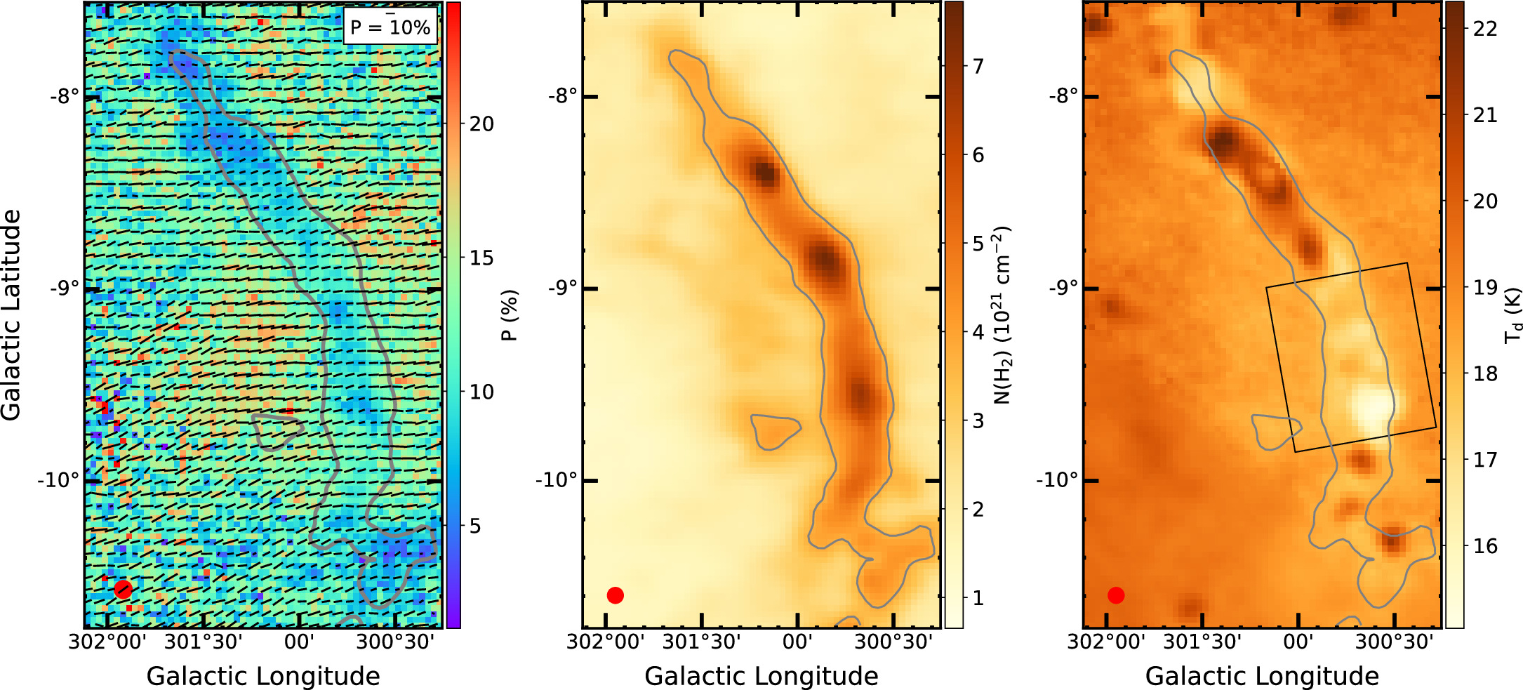
Figure 1. Musca observed by Planck. Left: B-field map. The length of the line segment is proportional to the polarization fraction P with a 10% reference. Center: column density. Right: dust temperature. The half-power beamwidth of the maps  is shown by the red circle in the lower left corner. The gray contours are 3.7 × 1021 cm−2. The black rectangle enclosing the southern section of the filament is the area of interest for further analysis.
Download figure:
Standard image High-resolution image
OMC-
1. The dust temperature and column density maps of OMC-1 are adopted from Chuss et al. (2019). These two maps were obtained by fitting SED from emission in the range of 53–35 mm, including data from SOFIA at 53, 89, 154, and 214 μm; Herschel at 70, 100, 160, and 250 μm; JCMT at 850 μm. The longest wavelength of the combined Green Bank Telescope and Very Large Array data at 3.5 and 35 mm was used to subtract the free–free emission caused by UV in the region. The final temperature and density maps have a resolution of 182. Those maps are shown in Figure 2 (center and right).
3. Data Analysis
To investigate the physics of dust alignment, the analysis of the polarization fraction and total intensity is frequently employed for simplification. However, total intensity is a function of column density and dust temperature, making it challenging to disentangle the effects of these two parameters from the polarization effect. Therefore, this study examines the relationship between the polarization fraction, P, gas column density, N(H2), and dust temperature, Td. Additionally, we analyze the variation of the angle dispersion function,  , to explore the impact of B-field tangling on dust polarization.
In the following subsections, we will first introduce Musca and OMC-1. Second, we will study the dependence of P on physical conditions, e.g., column density and dust temperature. This will reveal the basic properties of grain alignment and disruption in the regions. Then, we will present the dependence of P on the polarization angle dispersion function  to investigate the effects of the B-field tangling.
3.1. Musca
Musca (Figure 1) is located at a distance of 170 pc (Zucker et al. 2021). The filament is in its early evolutionary stage and lacks active star formation (Cox et al. 2016). One T Tauri star candidate is located at the end of its north (Vilas-Boas et al. 1994; in the galactic coordinates). Musca is known for being an isothermal filament in hydrostatic equilibrium and already fragmented; new stars can be formed in the near future (Kainulainen et al. 2016; Bonne et al. 2020). Polarization measurements from starlight (Pereyra & Magalhães 2004) and thermal dust emission (Cox et al. 2016; Planck Collaboration XXXIII 2016) show that local B-fields are generally perpendicular to the filament’s spine. Using Herschel data, Cox et al. (2016) found that B-fields follow the low-column density striations. It suggested that Musca has been accreting interstellar material through these low-column density striations. Recently, B-fields in a small part of the filament obtained by SOFIA/HAWC+ at higher spatial resolution also indicate that the B-field orientation is generally perpendicular to the filament’s spine (Kaminsky et al. 2023).
We use the polarization map from Planck at ∼850 μm (353 GHz). This is the highest frequency and most sensitive channel of Planck to dust polarization (Planck Collaboration XXXIII 2016). The Stokes I, Q, and U are mapped at the resolution of  corresponding to a physical scale of ∼0.24 pc. The pixel size of the maps is 112″. Musca is one of the high signal-to-noise ratio (S/N) regions of the Planck full-sky polarization map (Planck Collaboration XXXIII 2016). Figure 1 (left) displays the B-field map of Musca from Planck with the lengths of line segment proportional to the polarization fraction (P). The map is extracted from the Planck map and then reprojected to the galactic coordinates (using the reproject Python package of astropy).
Figure 1 (center and right) shows the N(H2) and Td maps obtained from the SED fitting by Planck Collaboration XI (2014). The density map reveals a nice filamentary structure with several fragments along the filament, and the column density increases from the filament’s outer to inner parts. The dust temperature map shows two trends in the filament’s spine: high temperature in the northern part ∼21 K and low temperature in the southern one <17 K. However, we note that the dust temperature of the filament from Planck data, which can go up to ∼22 K, is higher than that obtained by Herschel with a maximum Td of ∼18 K. Moreover, Bonne et al. (2020) reported using Herschel data that there is no high-temperature core as seen with the Planck temperature map (Figure 1, right). It should be noted that the Planck dust temperature is obtained based on six channels ranging from 20 to 3000 μm with a representative spatial resolution of  at 850 μm while for Herschel it is five channels ranging from 70 to 500 μm with much higher spatial resolution such as 36″ at 500 μm. The differences of the resulting Td maps may come from the different dust components probed by Planck and Herschel. Moreover, the high dust temperatures from Planck may be due to the confusion between the cold and warm components of the SED fitting (Lars Bonne in private communication). With Musca, we aim to study the nonembedded radiation source regions; for further studies, we only work with the southern part of the filament encompassed by the black rectangle in Figure 1 (right).
Planck Collaboration XXXIII (2016) conducted a detailed study of Musca using polarization data obtained by Planck. Their findings revealed a depolarization effect within the filament, manifesting as a drop in polarization fraction in the filament’s spine and a decrease in the polarization fraction with increasing gas column density. To understand the cause of the depolarization, we will examine the filament’s density, temperature, and B-field tangling. Due to its well-defined filamentary structure, we will explore the radial profiles of those quantities and their relations.
3.1.1. Gas Density Profile
We fit the radial density profile of Musca with a Plummer-like function using a Python package RadFil applied for a column density map (Zucker & Chen 2018; more details can be found in Appendix A.2). Assuming that the filament is in the POS, the Plummer-like function is as follows (Arzoumanian et al. 2011; Cox et al. 2016; Zucker & Chen 2018):
where r is the radial distance from the filament's spine; Rflat is the radius of the inner, flat region of the density profile; N(H2)(0) is the peak column density, and q is the power-law density exponent.
With the best-fit model given by RadFil, we find q = 1.94, and Rflat = 0.28 pc. Cox et al. (2016) fitted a Plummer-like function for Musca using Herschel data and obtained q = 2.2, and Rflat = 0.08 pc. Because Planck's beam size of ∼ (∼0.24 pc) is much larger than that of Herschel of ∼36″ (∼0.025 pc), our fitted Rflat is much larger than that of Herschel.
3.1.2. Filament Radial Profiles
Figure 3 shows the physical parameters across the filament obtained by RadFil, including the polarization fraction (a), polarization angle dispersion function (b), grain alignment efficiency  (c), and dust temperature (d).
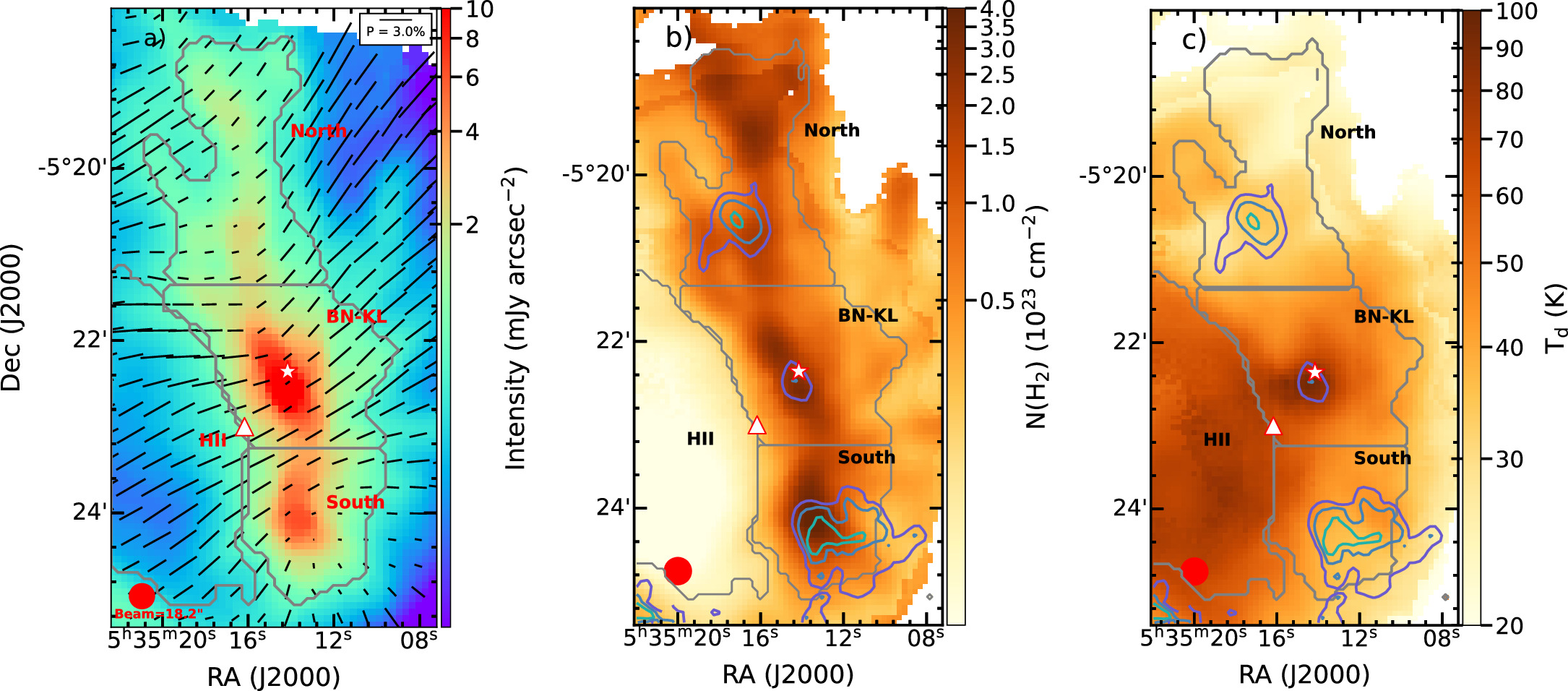
Figure 2. OMC-1. (a) B-field orientation map observed at 214 μm wavelength by SOFIA/HAWC+. The black lines show the orientation of the B-field vector and are overplotted on the intensity map. The vector spacing equals the beam size, shown by a solid red circle in the lower left corner. Three regions, north, BN-KL, and south, are labeled. (b) The column density map, and (c) the dust temperature map. The light green, dark blue, and violet contours correspond to P = 0.6%, 1.0%, 1.4%. The star indicates the location of BN-KL, and the triangle shows the location of the Trapezium cluster.
Download figure:
Standard image High-resolution imageIt is seen from the P profile (a) that P is the lowest in the filament's spine (∼8%). P increases to 15% at about 0.7 pc from the spine and then slightly decreases to 10% when going to the ISM. This trend is also found by Planck Collaboration XXXIII (2016; see their Figure 10).
To unravel the effects of B-field tangling on the decrease of P with decreasing r (depolarization), we analyze the polarization angle dispersion function,  , and the product
  shown in Figures 3(b) and (c).
  is generally low in Musca, and its mean value is smaller than 10°. Planck Collaboration XXXIII (2016) claim that this depolarization is not attributed to the B-field fluctuations because
  is small (∼10°), significantly smaller than 52° for random fields.
In addition to B-field tangling, the polarization fraction is influenced by environmental factors and alignment efficiency. Removing the effect of the B-field tangling,  represents the alignment efficiency of grains along the LOS (Planck Collaboration XII 2020). The
  radial profile reveals that the alignment efficiency is the lowest in the filament spine and increases when moving from the inner to the outer filament.
The temperature profile (d) shows that the temperature and column density (Figure A1) behave in the opposite manner; the temperature is low in the filament's spine, which has the highest density (∼5 × 1021 cm−2). The N(H2)–Td anticorrelation was also found with Herschel data by Bonne et al. (2020). The temperatures in the spine are below 18 K and can go down to 16 K. The mean temperatures increase from 17 to 20 K from the spine to the outer areas.
From those filament profiles, we see that the polarization fraction is lowest in the filament bone in which the temperature (or radiation field) is lowest, density is highest, and alignment efficiency is the lowest. The polarization fraction increases when the density decreases, dust temperature increases, and alignment efficiency increases.
3.2. OMC-1
Located at a distance of 388 ± 5 pc (Kounkel et al. 2017), the Orion Nebula is the nearest high-mass star formation region (O’dell et al. 2008). OMC-1 or Orion A is located behind an H ii region ionized by O-B stars from the Trapezium cluster. OMC-1 consists of two principal clumps, the northern Becklin–Neugebauer–Kleinmann–Low (BN-KL) clump (Becklin & Neugebauer 1967; Kleinmann & Low 1967) and the southern Orion S clump (Batria et al. 1983). BN-KL hosts an extremely explosive molecular outflow with a wide opening angle and multiple ejecta. B-fields of OMC-1 have an hourglass morphology and strengths of the order of mG (e.g., Pattle et al. 2017; Chuss et al. 2019; Guerra et al. 2021).
We use thermal dust polarization data observed toward the Orion BN-KL by SOFIA/HAWC+ at 214 μm and beam size of 182, which was first reported by Chuss et al. (2019). Analyzing this data set, Chuss et al. (2019) and later Guerra et al. (2021) mainly focused on the studies of B-fields. Chuss et al. (2019) found the depolarization effect. Evidence of RAT-D is found by Tram et al. (2021b) in BN-KL, and by Le Gouellec et al. (2023) in the Orion Bar. For the present work, we only use the data having S/Ns satisfying S/N(I) > 250 and S/N(P) > 3.
Figure 2 displays the maps of B-fields (a), column density (b), and dust temperature (c) observed toward OMC-1 by SOFIA/HAWC+ at 214 μm. We only consider the OMC-1 filament and H ii region encompassed by the gray contours. The H ii region has low column density of N(H2) < 2 ×1022 cm−2, and high dust temperature Td > 45K. While the filament has high column density N(H2) > 2 × 1022 cm−2 and strong emission I > 15  for a detailed study, we divided the OMC-1 filament into three subregions: north, BN-KL, and south.

Figure 3. Musca. Variations of P,  ,
,  , and Td as a function of the radial distance (r) constructed using RadFil by sampling radial cuts every 0.1 pc along the spine (similar to Figure A1). The radial distance is then defined as the projected distance; the negative distance is to the left, and the positive is to the right. Thin gray lines show the radial cuts, and the mean values are shown as dot makers per bin size of 0.1 pc.
Download figure:
Standard image High-resolution imageThe N(H2) map (Figure 2(b)) shows that the column density is highest in the filament's spine and divided into three clumps residing in the north, BN-KL, and south regions. BN-KL exhibits the highest temperatures, reaching 100 K (Figure 2(c)). The temperatures of the eastern part of OMC-1 and the H ii region are higher than that of the western one. This is due to the effect of ionization from the Trapezium cluster. The H ii region has the lowest densities compared to other regions.
The lengths of the line segments in Figure 2(a) are proportional to the polarization fraction, revealing high polarization fractions in the H ii region and particularly low polarization fractions in certain parts of the filament. The color contours in Figures 2(b) and (c) highlight three polarization holes in the central part of each subregion, with polarization fractions smaller than 1%. In Figures 2(b) and (c), the polarization holes in the north and south regions show lower dust temperatures compared to the polarization hole in BN-KL, despite all regions having high column density. This suggests that the depolarization in the low and high dust temperatures may be caused by different mechanisms.
To explicitly see how the polarization fraction, P, changes with the column density, N(H2), dust temperature, Td, and B-field tangling,  , we show the variations of P with N(H2), Td, and
  in Figure 4. The P−N(H2) relation (Figure 4(a)) shows an anticorrelation of the polarization fraction and the gas column density (i.e., polarization hole). We fit the data with a power-law model and obtain the power indices α = −0.33 ± 0.03 for north, α = −0.50 ± 0.01 for BN-KL, α = −0.45 ± 0.03 for south, and the smallest slope value α = −0.08 ± 0.01 for the H ii region. In the OMC-1 filament, the P–Td relation reveals that the polarization fraction increases at low Td and dramatically decreases as the dust temperature increases to Td > 70 K. In detail, the polarization fraction remarkably increases with increasing Td with a power index α = 2.82 ± 0.11 in the south, while in the north, with the low temperature (Td < 40 K), the polarization fraction slightly increases with α = 0.09 ± 0.08. In BN-KL, having massive protostars and a high dust temperature region, the polarization fraction only decreases as the dust temperature increases with α = −0.57 ± 0.06. Tram et al. (2021b) studied this relation for BN-KL using data collected by JCMT/POL-2 and SOFIA/HAWC+ and found this increase–decrease feature. Although dust temperature can go up to 80 K, the polarization fraction gradually increases with increasing Td in the H ii region with α = 0.41 ± 0.05.
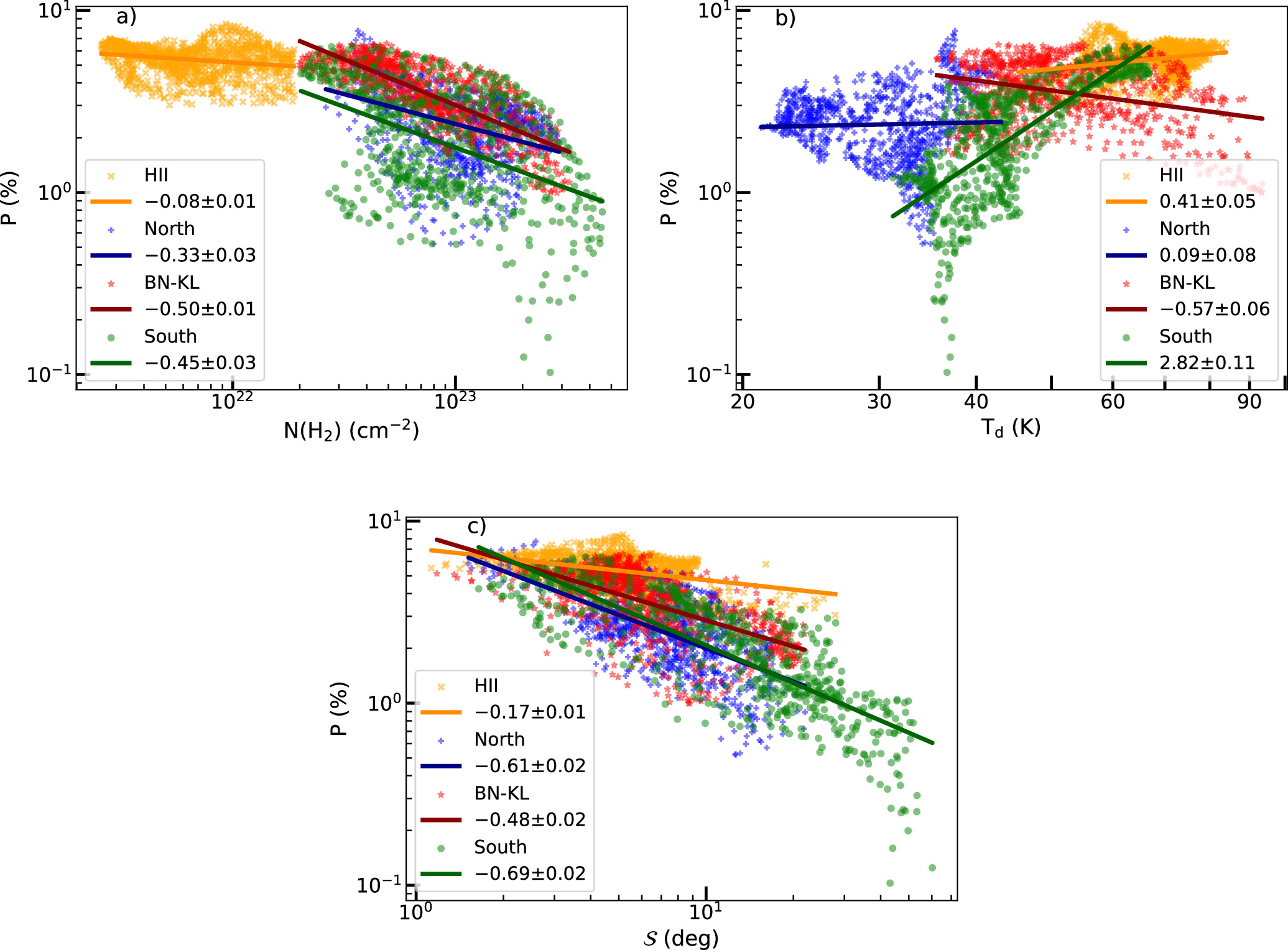
Figure 4. OMC-1. Variations of the polarization fraction, P, with the column density N(H2) (a), dust temperature Td (b), and angle dispersion function  (c). The blue, red, green, and orange dots represent the north, BN-KL, south, and the H ii region, and the lines are the results of fits to power-law models, respectively.
Download figure:
Standard image High-resolution imageWe also fit a power-law function to the  relation and find the anticorrelation of P and
  with α = −0.61 ± 0.02, −0.48 ± 0.02, −0.69 ± 0.02, and −0.17 ± 0.01 for north, BN-KL, south, and H ii region, respectively. The H ii region seems to have weak B-field fluctuations as shown by the small angle dispersion function of
  . However, the south region appears to have stronger B-field fluctuations due to the high angle dispersion function of
  .
.
From the N(H2)−Td relation shown in Figure 5(a), we see that N(H2)−Td is anticorrelated in the north, south, and H ii regions, while it is correlated in the BN-KL region with the presence of massive protostars. To show the effect of B-field tangling on the depolarization, we plot the relations of  and
and  in Figures 5(b) and (c). The
  relation shows the correlation of the polarization angle dispersion function
  and the column density in general. This clearly shows the increasing importance of B-field tangling in dense regions. The
  relation shows that the polarization angle dispersion function
  has anticorrelation with the dust temperature in the south and H ii regions, but a correlation in the north and BN-KL regions. The relationship between
  and Td (Figure 5(d)) shows that the average grain alignment efficiency first slightly increases with dust temperature for Td < 35K, remains constant in the range of 35–70 K, and then decreases for Td > 70 K.
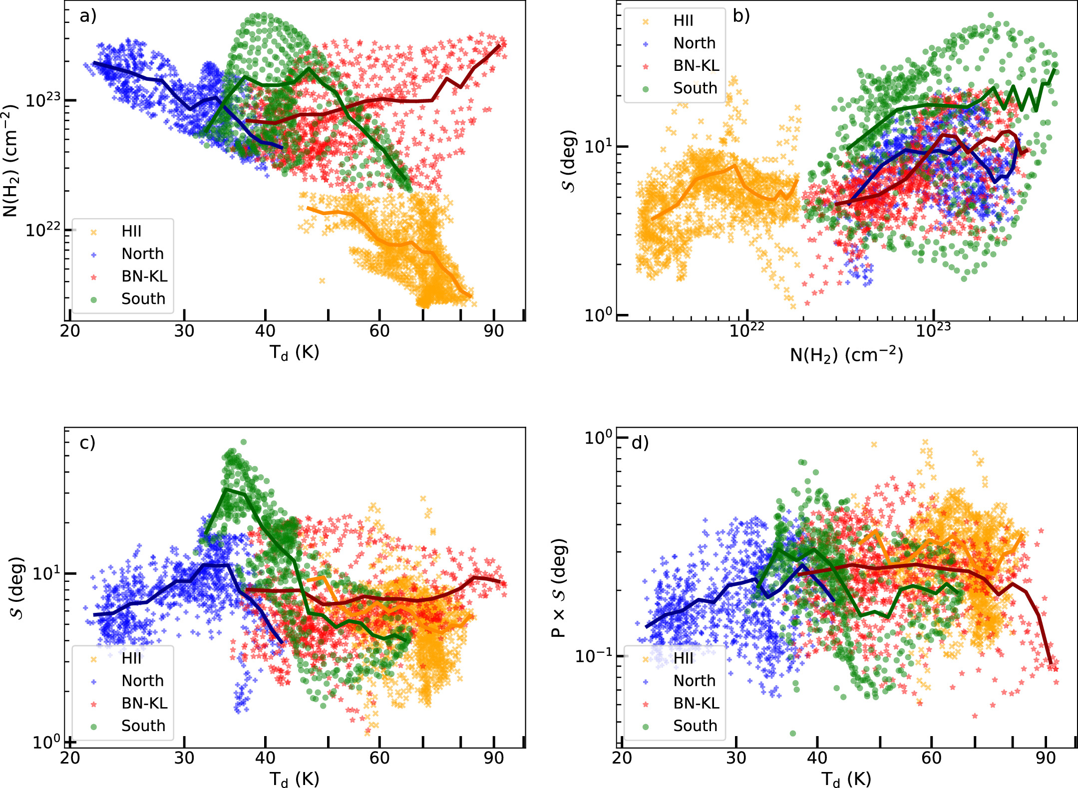
Figure 5. OMC-1. The dependence of column density on dust temperature (a), the angle dispersion function  on the column density N(H2) (b) and dust temperature Td (c), and the dependence of the
  on the dust temperature Td (d). The blue, red, green, and orange dots represent the data in the north, BN-KL, south, and the H ii regions, respectively, and the solid curves show the running mean values of the data.
Download figure:
Standard image High-resolution image4. Numerical Modeling and Results
This section presents the numerical modeling method of polarized thermal dust emission from aligned grains using the RAT theory for Musca and OMC-1 to test the RAT paradigm. We first use the DustPOL-py code, 6 which was first presented in Lee et al. (2020) and improved by Tram et al. (2021a) to obtain the dust polarization for the ideal model in which the B-fields are assumed to lie in the POS. Then, we incorporate the depolarization effects caused by the B-field inclination angle and their fluctuations into our ideal model to obtain a realistic polarization model and confront it with observational data.
Below, we briefly describe the main features of DustPOL-py and its key input parameters, including the physical parameters of the gas and dust, the local radiation field, and the alignment of dust grains by RATs. We then present the main modeling results and compare them to the data. Our modeling approach is physical modeling based on the alignment physics of RATs. There exist other polarization modeling approaches, such as inverse modeling (Kim & Martin 1995; Draine & Allaf-Akbari 2006; Hoang et al. 2013) and parametric modeling (Guillet et al. 2018; Hensley & Draine 2023). However, the latter two modeling methods are not based on underlying physics and require multiwavelength data to derive model parameters; therefore, they are not convenient for pixel-by-pixel modeling with single-wavelength data, which we do in the present study.
4.1. Methods and Assumptions
4.1.1. Gas Properties and Radiation Fields
The gas density ( ) and temperature (Tgas) are the two important physical parameters in the RAT alignment theory because they determine the randomization and alignment of dust grains (see, e.g., Hoang et al. 2021). For our modeling, these parameters are inferred from observational data and used as the input parameters for DustPOL-py .
For radiation fields, the radiation strength, U (effectively equivalent to the dust temperature Td) and the anisotropy degree of the radiation, γ, are the key parameters of the RAT theory because they determine the alignment degree of dust grains (Hoang et al. 2021). The anisotropy degree varies in a range from 1 to 0; γ = 1 represents a unidirectional radiation field from a nearby star, while γ = 0.1 for the diffuse ISM (Draine & Weingartner 1996). The mean wavelength,  , depends on specific regions.
4.1.2. Grain Size Distribution
We adopt a power-law grain size distribution,  , where β is in the range of 3.5–4.5. The grain size distribution in the ISM follows the Mathis-Rumpl-Nordsieck distribution with a power-law index β = 3.5 (Mathis et al. 1977). The smallest grain size,
  , is 10 Å, while the initial maximum grain size,
  , can be varied in the range of 0.2 μm to several microns.
When considering the RAT-D effect, the value of  varies with the local conditions of the gas densities, radiation fields, and tensile strengths, as given by Equation (A4). Their tensile strengths determine the internal structure of grains, and the disruption temperature depends on this property. For composite grains, the tensile strengths vary around
  (Hoang 2019).
4.1.3. Grain Alignment Function by RATs
In the RAT-A theory, grains are first spun up to suprathermal rotation and then driven to be aligned with the ambient B-fields by RATs (Lazarian & Hoang 2007; Hoang & Lazarian 2008). For grains with iron inclusions, which are superparamagnetic material, the joint effect of enhanced magnetic relaxation and RATs could make grains achieve perfect alignment with B , a mechanism known as magnetically enhanced RAT (MRAT. Hoang & Lazarian 2016). Therefore, grains are only efficiently aligned when they can rotate suprathermally. The minimum size for grain alignment, aalign (also called critical alignment size), is determined by the suprathermal rotation criterion of ωRAT(aalign) = 3ωT (Hoang & Lazarian 2008), where ωRAT(aalign) is the angular velocity of grains spun up by RATs, and ωT is the grain's thermal angular velocity. From Equation (A1), one can obtain
where U is the radiation strength of the local radiation field (Hoang et al. 2021).
The degree of grain alignment as a function of the grain size can be described by

where aalign is given by Equation (11),  describes the maximum degree of grain alignment, and the negligible alignment of small grains of a ≪ aalign is disregarded (Hoang & Lazarian 2016).
According to the MRAT mechanism, the exact value of  depends on the ratio of the magnetic relaxation to the gas damping rate, which is a function of the grain size, magnetic susceptibility, and local gas density, as shown in Hoang & Lazarian (2016). They also numerically demonstrated that grains with embedded iron clusters (i.e., superparamagnetic grains) can achieve perfect alignment of
  . Moreover, inverse modeling of thermal dust polarization observed by Planck in Hensley & Draine (2023) found that perfect alignment of large grains is required to reproduce the observational data. Therefore, in this paper, we assume
  , which is expected from the MRAT theory for composite grains containing embedded iron inclusions.
4.1.4. Ideal Model of Thermal Dust Polarization with DustPOL-py
Dust grains are heated by starlight and subsequently reemit radiation in infrared wavelengths. In the assumption of a dust environment containing both carbonaceous and silicate grains, the total emission intensity is calculated as
where Qabs is the absorption efficiency, dP/dT is the temperature distribution function, and Bλ (Td) is the Planck function. Here, we disregard the minor effect of grain alignment on total emission intensity (see Hoang & Truong 2024).
If carbonaceous and silicate grains exist in two separate populations, only silicate grains can be aligned with B-fields due to their paramagnetic nature, while carbonaceous grains (e.g., pure graphite) cannot be efficiently aligned because of their diamagnetic nature (Hoang & Lazarian 2016). 7 However, for a composite dust model (a mixture of silicate and carbon in a dust grain), the composite dust can be aligned with B-fields. Note that observational constraints favor the composite model for interstellar dust, such as Astrodust (Draine & Hensley 2021) and THEMIS model (Ysard et al. 2024). Hence, for this study, we assume the composite dust model, so that carbonaceous and silicate grains have the same temperature.
We consider first the ideal model in which B-fields lie in the POS, and the impact of B-field fluctuations is disregarded. The polarized emission intensity from aligned grains is then given by

where Qpol is the polarization efficiency (Lee et al. 2020).
The polarization degree of thermal dust emission is given by

where the subscript “mod” is for the values calculated from the model and superscript “ideal” for the ideal polarization degree achievable by grain alignment, assuming the optimal case of B-fields in the POS with the absence of the B-field tangling.
4.1.5. Realistic Polarization Model: Accounting for B-field Tangling
For DustPOL-py, B-fields are assumed to lie in the POS, so that the degree of thermal dust polarization could achieve the maximum value, as given by Equation (15). In a realistic situation, the inclination angle of B-fields and LOS, denoted by ψ, contributes to the polarization degree due to the projection effect. Moreover, the fluctuations of B-fields along the LOS cause the depolarization of thermal dust emission, which is described by an additional depolarization parameter Fturb. Fturb is a function of the angle between the local B-field and the mean B-field and is anticorrelated with the polarization angle dispersion function  (Hoang & Truong 2024). Therefore, the realistic dust polarization degree becomes

Numerical simulations in Hoang & Truong (2024) using MHD simulations and polarized radiative transfer in POLARIS found that the polarization model given by Equation (16) is in excellent agreement with synthetic polarization. They also found that Fturb decreases with  as
as  , where η1 depends on the inclination angle. Numerical simulations in Planck Collaboration et al. (2015) showed that there is a correlation between the average of the B-field inclination angle and
  , which can be described as
  (see, e.g., Hensley et al. 2019). Furthermore, the B-field tangling within the beam size (i.e., B-field fluctuations in the POS) can cause an additional depolarization described by the factor Fbeam (Hoang & Truong 2024). Accounting for all these depolarization effects, the net polarization degree of thermal dust emission can be described by

where Φ is a coefficient that describes the depolarization by the B-field’s inclination angle, and η > 0 is the power index describing the depolarization effect caused by B-field fluctuations along the LOS and in the POS, which is expected to vary with the local conditions. In practice, we get the value of η from the slope of the  relation. The value Φ is obtained by fitting the polarization fraction from the model to the maximum polarization observed in each filament. The best-fit values of Φ are shown in Table 2.
Table 2. Physical Parameters for Model
| Parameter | Musca | OMC-1 | |
|---|---|---|---|
| Anisotropic degree | γ | 0.3 | 1 |
| Mean wavelength |
![$\bar{\lambda }\,[\mu {\rm{m}}]$](https://content.cld.iop.org/journals/0004-637X/974/1/118/revision1/apjad6a5eieqn67.gif)
| 1.2 | 0.3 |
| Gas temperature | Tgas [K] | Td ust | Tdust (filament), 5000 K (H ii region) |
| Grain composition | ⋯ | Sil+Car | Sil+Car |
| Dust mass density | ρ [ g cm−3] | 3 | 3 |
| Minimum grain size |
![${a}_{\min }\,[\mu {\rm{m}}]$](https://content.cld.iop.org/journals/0004-637X/974/1/118/revision1/apjad6a5eieqn68.gif)
| 10−3 | 10−3 |
| Maximum grain size |
![${a}_{\max }\,[\mu {\rm{m}}]$](https://content.cld.iop.org/journals/0004-637X/974/1/118/revision1/apjad6a5eieqn69.gif)
| 0.25−0.5 | 0.2−2 |
| Power index | β | −3.5 | −3.5 |
| Maximum tensile strength |
 [erg cm−3] [erg cm−3] | 107 | 107−108 |
| B-field’s inclination effect | Φ | 0.53 | 0.28 |
Download table as: ASCIITypeset image
4.2. Results
Table 2 summarizes the model parameters for Musca and OMC-1, including the gas number density, nH, gas temperature, Tgas, ( ,
,  ), shape (grain aspect ratio = minor axis/major axis taken to be equal to 1/3), size distribution power index, β, tensile strength,
  , radiation field strength, U, the mean wavelength,
  , and the anisotropy degree, γ.
4.2.1. Musca
In Musca, where a filamentary structure is evident, and the physical conditions do not vary significantly along the filament, we will model the variation of polarization faction P across the filament, as the function of the radial distance, r, from the filament’s spine to the outer regions.
To model the dust polarization as a function of the radial distance, r, we first need to know how the local gas volume density and dust temperature (radiation field) vary with r. The dust temperature profile is taken to be the mean temperature obtained from Planck (Figure 3(d)).
For the regions of ∣r∣ < 1 pc within the filament, the gas number density varies with the radial distance r as the Plummer-like function (e.g., Arzoumanian et al. 2011),

where  is the number density at the filament center r = 0, given by

where

with i as the inclination angle of the filament relative to the POS, and we assumed i = 0. Following Plummer-like fitting as described in Section 3.1.2, we obtain  .
.
For the outer regions of ∣r∣ > 1 pc, we assume a constant gas density of  and constant dust temperature of Td = 18.3 K (Figure 3(d)).
Figure 6 (upper panel) shows the variation of the minimum alignment size by RATs (aalign) computed for Musca. The alignment size increases rapidly toward the filament spine due to the increase in the gas volume density and reduction of the radiation field (dust temperature). For a fixed maximum size,  , the increase in aalign corresponds to the increasing loss of grain alignment of grains having sizes smaller than aalign toward the filament’s spine.
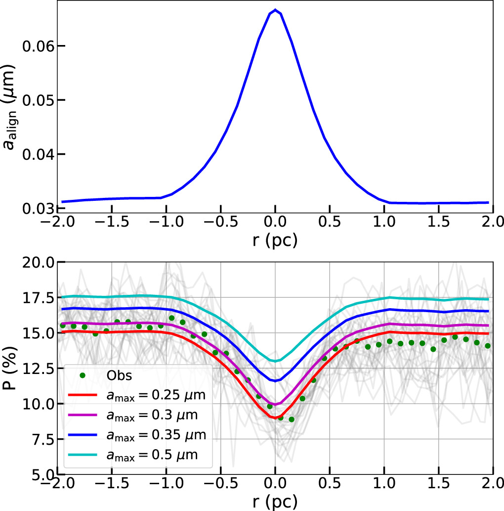
Figure 6. Musca. Upper: minimum alignment size by RATs calculated from our model for Musca. Lower: comparison of the polarization fraction from our model (thick solid lines) with observation data. The gray curves show P vs. r for radial cuts along the filament’s spine from observational data (see Section 3.1.2). Green dots represent the mean values of the observational P at a certain value of r. The color curves show polarization fractions from our model with different  . The rapid increase of alignment size toward the filament center causes the decrease of the model polarization fraction and successfully reproduces the observed polarization hole.
Download figure:
Standard image High-resolution imageFigure 6 (lower panel) compares the polarization profile obtained from our modeling,  , given by Equation (17), with the observational data for the case without RAT-D. Musca has low temperatures <19 K and high densities of 102–103 cm−3; therefore, RAT-D cannot occur. Models with only RAT-A can very well reproduce the data. We note that the B-field tangling is expected to have a minor effect on the polarization hole in Musca because the values of polarization angle dispersion function
  are small (<10°) and do not change considerably across the filament (Figure 3(b)). In addition, there is little dependence of P on
  with η = 0.03.
Figure 6 shows model predictions of the polarization fraction with different values of maximum grain sizes varying from 0.25 to 0.5 μm. Dust grains can be aligned between aalign and  therefore, higher
  produces a higher polarization fraction. Moreover, as
  increases, the size distribution of aligned grains becomes broader, narrowing the difference between the polarization fraction between the outer and inner of Musca. As shown, our polarization models with
  can successfully reproduce the strong decrease in the polarization fraction toward the filament’s spine. Therefore, the loss of grain alignment by RATs (i.e., increasing aalign) toward the denser and colder region of the filament (upper panel) is the main origin of the polarization hole observed in Musca.
4.2.2. OMC-1
For OMC-1 that has the structure and physical conditions varying significantly, such as between the east and west (with/without H ii region) and the presence/absence of an embedded protostar within the filament, we will perform pixel-by-pixel modeling for the whole region to obtain maps of the polarization fraction to compare with the observational data.
For the modeling of the OMC-1 molecular cloud, we assume the mean radiation wavelength to be  (Hoang et al. 2021), which corresponds to
  for the presence of the nearby massive OB star cluster of T⋆ > 2 × 10⁴ K. The pixel-by-pixel maps of the number density,
  , and dust temperature, Td, are used for modeling grain alignment and polarization fraction. To derive the number density map, OMC-1 is assumed to have the same depth dOMC = 0.15 pc, as obtained by Chuss et al. (2019). Therefore, the volume density is accordingly calculated by
  . To reduce measurement noise and optimize model computation time, we increase the pixel size by a factor of ∼4 to be 14″, almost equal to the spatial resolution of the input data maps.
Since grain growth is expected to be efficient in dense star-forming regions, we assume the maximum grain size of  for N(H2) > 2 × 10²² (cm−2) in OMC-1. In the remaining regions of low density, such as the outer region of the filament structure, and the H ii region, we assume the maximum grain size of
  , similar to that of the diffuse ISM. When modeling the RAT-D effect expected to be important in OMC-1 due to strong radiation fields, the tensile strength of dust grains is required. Because the tensile strength of dust grains depends on the grain internal structure (e.g., porosity), which varies with the grain size due to grain coagulation (Tatsuuma et al. 2019), we assume
  for large grains having
  , and a higher tensile strength of
  for grains having
  .
.
As shown in Figure 4(c), the angle dispersion function in OMC-1 can go up to 50°, and the slopes of  relation are 0.47–0.69 in the filament, which means that B-field tangling in OMC-1 is stronger than Musca and varies significantly across the object. Therefore, one cannot take the dust polarization results directly obtained by DustPOL-py as in Musca. We use the polarization model, which takes into account the effect of B-field fluctuations given by Equation (17) for different subregions in OMC-1 with different η (see Section 4).
Figures 7(b)–(e) show the polarization fraction maps obtained by using our numerical modeling. Figure 7(a) shows the observational data for comparison. We note that the pixel sizes in Figure 7 now are ∼14″. From Figure 7(b), one can see that  without RAT-D can reproduce a part of the south and north polarized holes; however, the model cannot reproduce the polarization hole in BN-KL. Figure 7(c) shows the result from
  with RAT-D; the polarization fraction decreases in the BN-KL region, but P from the model is significantly higher than the observed data. The models in Figures 7(d) and (e) incorporate B-field tangling effects,
  without/with RAT-D with exponents η = 0.61, 0.48, 0.69, and 0.17 for the north, BN-KL, south, and H ii regions, respectively. Here, the values of η are chosen based on the slopes of the
  relation in Figure 4(c). It is evident that
  without RAT-D is limited to reproducing observations in the southern and northern areas. However, when RAT-D is incorporated, our model aligns more closely with observations, including those in the BN-KL and H ii regions. In the ensuing analysis, we conducted a thorough comparison utilizing two distinct diagnostic methods for the P–Td relationship (which directly reflect the impact of alignment and disruption) and P−N(H2) (which directly reflects the gas damping effect).
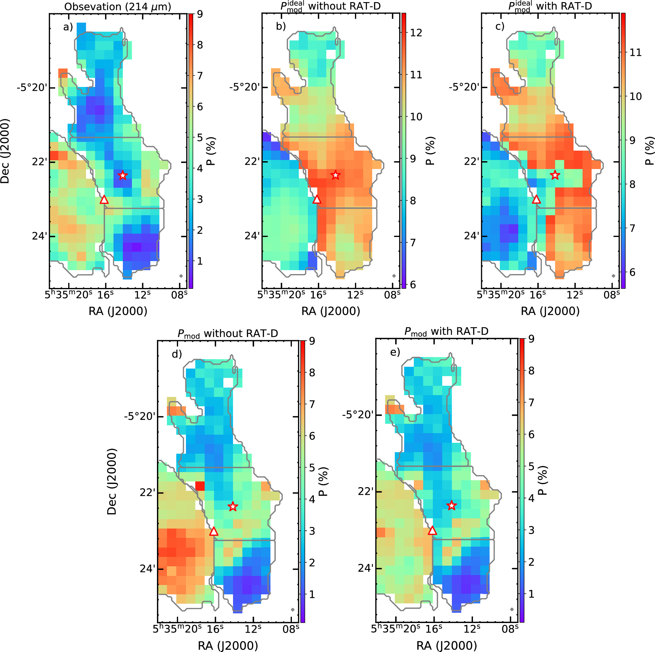
Figure 7. OMC-1. The polarization fraction maps, (a) from observation and (b)–(e) from numerical modeling: (b)  without RAT-D, (c)
  with RAT-D, (d)
  without RAT-D, and (e)
  with RAT-D. The gray contour corresponds with four subregions defined in Figure 2. The star indicates the location of BN-KL, and the triangle shows the location of the Trapezium cluster.
Download figure:
Standard image High-resolution imageFigure 8 shows the comparison of the P–Td relation produced by our model and from observations for the whole OMC-1. There is a noticeable correlation between P and Td at low temperatures (<70 K), while an anticorrelation is observed at high temperatures (>70 K). It is clear that models that do not take into account the fluctuations of B-fields fail to reproduce the observations, while those incorporating both the RAT-D mechanism and B-field fluctuations provide the most satisfactory explanation for these two trends compared to other models.
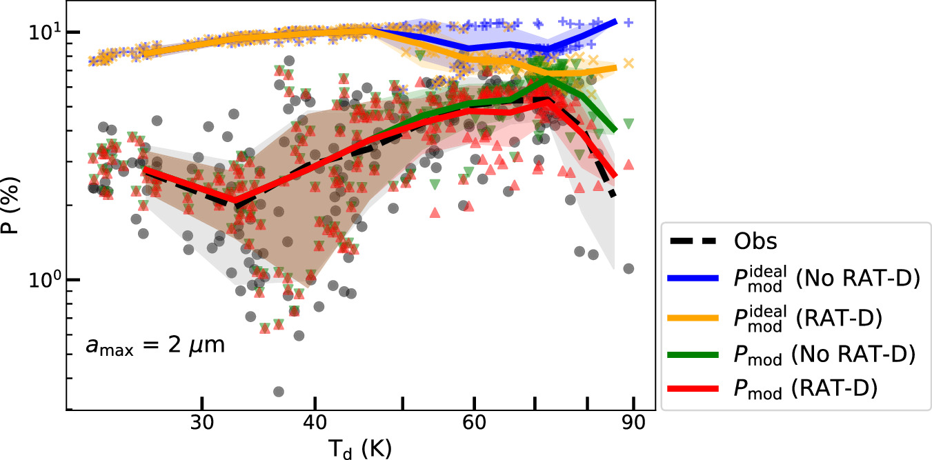
Figure 8. OMC-1. Comparison of the polarization degree vs. dust temperature relation from our models (color lines) with observational data (black line). The shaded area represents the 1σ deviation of each bin of data points, which are shown by points (black for observation data and color for model data). The ideal polarization model overestimates the observational data (blue and orange lines), but the realistic polarization model (red line) considering RAT-A, RAT-D, and B-field tangling ( ) can best reproduce the observed variation of P–Td.
Download figure:
Standard image High-resolution imageFigure A2 shows the comparisons for the individual regions, including the north, south, BK-KL, and H ii regions. In the regions with lower dust temperatures (north and south), models with only RAT-A and a combination with RAT-D are identical because the disruption effect does not occur. For the regions of high dust temperatures (BN-KL and H ii), models with RAT-D and B-field fluctuations best reproduce the decrease of polarization degree at Td > 50 K.
Figure 9 compares the P−N(H2) relations of our models with observations. One can see that models without B-field tangling,  , produce a rather high polarization and cannot reproduce the polarization hole. On the other hand, models with the B-field tangling,
  , better reproduce the data. Therefore, the main cause of the depolarization in P−N(H2) is due to the B-field tangling, and the grain alignment is still efficient at a large column density due to the effect of embedded radiation sources. This is different from the case of Musca, where the main cause of the polarization hole is the loss of grain alignment toward the denser and weaker radiation field.
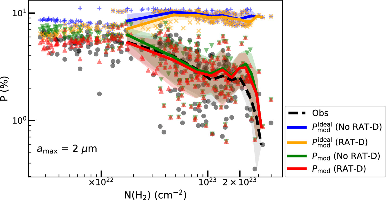
Figure 9. OMC-1. Same as Figure 8 but for P−N(H2) relation. The ideal polarization model (blue and orange lines) cannot reproduce the data, but the realistic polarization model (red line) considering RAT-A, RAT-D, and B-field tangling ( ) can best reproduce the observed polarization hole.
Download figure:
Standard image High-resolution imageWe refer to Table 3 for a quantitative χ2 comparison. As shown, the values of χ2 are larger for  and smaller for
  with the RAT-D effect. It is improved for the BN-KL and H ii regions where RAT-D happens.
  with the B-field tangling produces the smaller χ2, which implies that both grain alignment and B-field tangling play a role in the observed polarization. Therefore, we see that the best model is
  with both RAT-D and B-field tangling taken into account.
Table 3. The Comparisons between Models and Observations for Different Regions in OMC-1: North, BN-KL, South, H ii, and All
| Model | χ2 | ||||
|---|---|---|---|---|---|
| North | BN-KL | South | H ii | All | |
 without RAT-D without RAT-D | 21.65 | 17.34 | 46.77 | 1.39 | 18.76 |
 with RAT-D with RAT-D | 21.65 | 12.24 | 45.88 | 0.65 | 17.20 |
 without RAT-D without RAT-D | 0.32 | 0.83 | 0.30 | 0.32 | 0.43 |
 with RAT-D with RAT-D | 0.32 | 0.55 | 0.4 | 0.17 | 0.34 |
Note. The statistical evaluation is shown by  with N the number of pixels within each region. As shown, the values of χ2 are the highest for
  .
.  with B-field tangling and RAT-D produces the smallest χ2, which implies that both grain disruption and B-field tangling play an important role in the observed polarization. Moreover, the model with the rotational disruption effect matches much better with observations in BN-KL and H ii regions.
Download table as: ASCIITypeset image
5. Discussions
In this section, we will discuss the evidence of grain alignment and disruption by RATs obtained from comparing modeling results with observational data for Musca and OMC-1.
5.1. Evidence of RAT-A Mechanism
5.1.1. Decrease of Polarization Fraction with Column Density: Origin of Polarization Hole
The anticorrelation between P and N(H2) (or Av), aka the polarization hole, is usually found in various environments, from the diffuse ISM to molecular clouds, filaments, and star formation regions (e.g., Pattle & Fissel 2019). Yet, the exact origin of the polarization hole remains unclear. The loss of grain alignment toward denser regions by RATs is a leading explanation for the polarization hole (Hoang et al. 2021). Qualitatively, according to the RAT-A theory, grains are only efficiently aligned with B-fields if the grain size is larger than the minimum alignment size of  (see Equation (11)). The alignment size increases with increasing gas density and decreasing Td, leading to a narrower size distribution of aligned grains and the lower dust polarization fraction (Lee et al. 2020).
In this paper, to quantitatively test the RAT-A theory, we analyzed the thermal dust polarization data toward one of the simplest filaments, Musca, that exhibited a clear polarization hole. We performed a detailed polarization modeling for Musca using the local volume density and radiation fields (dust temperatures) from observational data as the input parameters for the DustPOL-py code. Our modeling results showed that the alignment size (aalign) increases rapidly from the outer to inner filament when the density increases, and the dust temperature decreases (see upper panel of Figure 6). As a result, the polarization degree (P) decreases rapidly toward the filament spine, successfully reproducing the polarization hole observed toward Musca (see the lower panel of Figure 6).
5.1.2. Increase of Polarization Fraction with Dust Temperature
The second prediction of the RAT-A mechanism is the increase of the polarization degree with increasing dust temperature because the alignment size decreases with Td (see Equation (11)), and the size distribution of aligned grains becomes broader (Lee et al. 2020).
For both filaments, the polarization data indeed show the increase of P with Td for low temperatures (see Section 3). However, for OMC-1 with strong radiation fields, the polarization degree reverses its trend at sufficiently high temperatures, which suggests the signature of RAT-D. Our detailed modeling for Musca and OMC-1 successfully reproduce the rising trend of P–Td (see Figures 10 and 11).
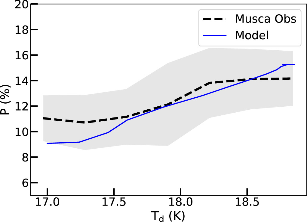
Figure 10. Musca: comparison of the polarization degree vs. dust temperature relation from our models (blue line) with observational data (black line). The shaded area represents the 1σ deviation of each bin of data points. The observed increase of P with Td can be successfully reproduced by the polarization model based on the RAT-A theory.
Download figure:
Standard image High-resolution image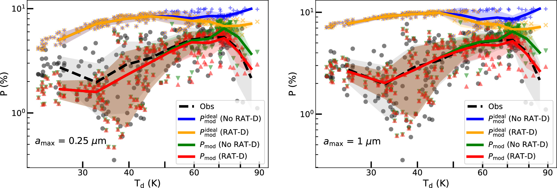
Figure 11. OMC-1. Comparison of the polarization fraction between our models and observations for different initial maximum sizes of  (left panel) and
  (right panel). The latter realistic models (red line) can reproduce better the data for the region of high density but low temperatures of Td < 50K, revealing the significant grain growth in this dense region.
Download figure:
Standard image High-resolution image5.1.3. Role of B-field Tangling in Producing Polarization Hole: The Anticorrelations of  and P versus N(H2)

Together with grain alignment and properties, the polarization fraction, P, also depends on the fluctuations of B-fields along a light of sight and within the beam (Hoang & Truong 2024). The polarization angle in the POS is the average of the polarization patterns, which are aligned with the local B-fields along an LOS. Therefore, polarization angle dispersion function  is usually used to describe the B-field fluctuations.
In Musca, where the B-field fluctuations are small (see Figure 3), our polarization model based on the RAT paradigm could reproduce the observed polarization data (see Figure 6). Therefore, the loss of RAT alignment is the main cause of the polarization hole, and the effect of B-field tangling is negligible.
The situation becomes different for OMC-1, where B-field fluctuations are strong and spatially dependent (see Figure 5). Our detailed modeling results show that the model without B-field tangling,  , produces too high polarization and cannot reproduce the data. Only the polarization models including B-field tangling effects,
  , could reproduce the observational data (see Figure 8). This reveals the important role of B-field tangling in producing the polarization hole in OMC-1.
5.2. Evidence of RAT-D Mechanism in OMC-1
The correlation of P and Td at low dust temperature and anticorrelation at high dust temperature is found in the OMC-1 filament. The decreasing trend at high dust temperature is the opposite of what would be expected from the RAT-A theory, but a signature of RAT-D.
To quantitatively study whether RAT-D could reproduce the declining trend in OMC-1, we performed detailed modeling of dust polarization using the maps of the gas volume density and dust temperature for each pixel obtained from observations. Our modeling results could reproduce the P versus Td relation (see Figure 8).
We note that the B-field tangling ( ) alone cannot reproduce the decrease of P with Td at high temperatures. Indeed, as shown in Figure 5, the polarization angle dispersion function
  tends to decrease or change slowly at high Td. Our models that take into account both the B-field tangling and RAT-D shown in Section 4 could produce the observed P–Td relation at high Td. Therefore, the RAT-D effect can explain the decreasing trend of P–Td in OMC-1.
In previous simple modeling and data analyses using SOFIA/HAWC+, tentative evidence of RAT-D in some regions of OMC-1 was reported, e.g., in BN-KL region (Tram et al. 2021b) and in Orion Bar (Le Gouellec et al. 2023). It is worth noting that evidence of RAT-D was previously found in several star-forming regions: Auriga (Ngoc et al. 2021), Oph A (Tram et al. 2021a), 30 Doradus (Tram et al. 2021c), and M17 (Hoang et al. 2022).
5.3. Implication for Probing Grain Growth
Observational studies suggest that the upper limit of the grain size distribution in the ISM is ∼0.25 μm (Mathis et al. 1977). However, grain growth is expected to occur within dense molecular clouds or filaments due to gas accretion and grain coagulation. Vaillancourt et al. (2020) reveal grain growth in dense clouds using observations of starlight polarization combined with numerical modeling using the RAT theory. Using polarization data, Ngoc et al. (2023) gives evidence that grain growth is moderate with  in the G11 filament when the volume density is higher than 104 cm−3.
In this study, our numerical modeling for Musca shown in Figure 10 reveals that the maximum grain size is ∼0.3−0.35 μm. This implies grain growth is effective but not significant in this not-dense filament, with the highest density of nH ∼ 103 cm−3. On the other hand, the density of the OMC-1 filament varies significantly and can reach a high value of 104−106 cm−3. To probe grain growth in this dense filament, we varied  from 0.2 to 2 μm and found that the model with
  can well reproduce the P–Td relation, in particular the low Td region in the lower dust temperature, Td < 50 K (see Figure 11, left). This suggests that grain growth is significant in the dense regions of OMC-1.
5.4. Limitations of Our Modeling and Future Works
In this paper, we have used the hybrid approach to perform modeling of thermal dust polarization and test the RAT paradigm. We first used the DustPOL-py code to calculate the polarization fraction predicted by the RAT theory for the ideal model with B-fields in the POS. To account for the effects of the inclination and the tangling of B-fields, we then incorporated a coefficient Φ to describe the inclination angle and a depolarization factor  to describe the effect of B-field fluctuations (Equation (17)). The final realistic dust polarization model is based on the optically thin assumption, which is successfully tested with synthetic observations of MHD simulations using POLARIS in Hoang & Truong (2024). Although our numerical modeling can successfully reproduce the observational data and support the RAT paradigm, there are several limitations. First, we have assumed that grains are aligned via the MRAT mechanism with
  , which is expected for grains with embedded iron clusters. Second, the coefficient Φ obtained by fitting the polarization model to the maximum observed polarization is assumed to be constant across the filament. Such an assumption is likely valid for Musca, which has well-ordered B-fields and a small slope η ∼ 0.03. However, it may not be realistic for a complex star-forming region like OMC-1, which has strong B-field fluctuations, and the slope η is found to vary considerably from region to region in OMC-1.
In our follow-up studies, we will perform synthetic dust polarization using MHD simulations with our updated POLARIS code (Giang et al. 2023), which includes both the RAT paradigm and the radiative transfer process. A detailed comparison of synthetic simulations with observational data would help disentangle the different origins of the polarization hole in filaments, including grain alignment loss, disruption, and B-field tangling.
6. Conclusions
In this study, we utilize dust polarization data observed toward Musca and Orion to test the grain alignment and rotational disruption mechanisms by RAT (i.e., RAT paradigm). We investigate the relation of the polarization degree, P, with gas column density, N(H2), and dust temperature, Td, and compare them with theoretical predictions using the RAT paradigm. Additionally, the variation of P with polarization angle function,  , is explored to study the effects of B-field fluctuations. Our results are as follows:
- 1.Observational data show the existence of a polarization hole, i.e., the decrease of the polarization degree with increasing the gas column density in both Musca and OMC-1. The analysis of the observed polarization angle dispersion reveals that B-fields fluctuations are rather weak in Musca but strong in OMC-1.
- 2.For Musca with weak B-field fluctuations, our detailed modeling of dust polarization using the RAT theory with small B-field tangling effects succeeds in reproducing the polarization hole, suggesting the loss of RAT alignment as the main cause of the polarization hole in this filament. Moreover, our modeling results show that grain growth is effective but not significant in Musca.
- 3.For the high-mass star-forming region, OMC-1, we find that, in general, polarization fraction (P) and polarization angle dispersion function () are anticorrelated, but N(H2) and are correlated, especially at low temperatures. This trend suggests that the B-field fluctuations in dense regions dominantly contribute to the depolarization effect.
- 4.Observational data exhibited a general correlation of P with Td at low temperatures, such as in the northern and southern. In the Orion BN-KL region of high temperatures, P reverses the trend and decreases with Td.
- 5.Using the pixel-by-pixel polarization modeling method with local physical parameters (gas density and radiation fields) inferred from observations as the input, we demonstrate that the observed P–Td and P−N(H2) (polarization hole) relations can be simultaneously reproduced by our polarization models incorporating both RAT-A and RAT-D, and the contribution of B-field fluctuations. The decreasing trend of P–Td when taking into account the RAT-D effect from models is in agreement with observations from the BN-KL region.
- 6.The successful testing of the RAT paradigm through the combination of pixel-by-pixel polarization modeling using DustPOL-py with observational data to two different filaments of quiescent one (Musca) and an active star-forming region (OMC-1) opens the avenue for testing the RAT paradigm and constraining dust properties in other astrophysical environments.


Acknowledgments
The authors greatly appreciate the anonymous reviewer for carefully reading the manuscript and providing valuable comments and suggestions. The authors sincerely thank Dr. Hyeseung Lee for her help with DustPOL-py in the initial stage of this work. We thank Dr. Lars Bonne for discussions regarding the Planck data, Dr. Joseph Michail and Prof. David Chuss for sharing the thermal dust polarization, dust temperature, and gas column density of OMC-1. This research was funded by Vingroup Innovation Foundation under project code VINIF.2023.DA.057. T.H. is supported by a grant from the Simons Foundation to IFIRSE, ICISE (916424, N.H.). N.B.N. was funded by the Master, Ph.D. Scholarship Programme of Vingroup Innovation Foundation (VINIF), code VINIF.2023.TS.077. This research is based on observations made with the NASA/DLR Stratospheric Observatory for Infrared Astronomy (SOFIA). SOFIA is jointly operated by the Universities Space Research Association, Inc. (USRA), under NASA contract NNA17BF53C, and the Deutsches SOFIA Institut (DSI) under DLR contract 50 OK 0901 to the University of Stuttgart. This work is based on observations obtained with Planck (http://www.esa.int/Planck), an ESA science mission with instruments and contributions directly funded by ESA Member States, NASA, and Canada.
Facilities: - SOFIA, Planck - European Space Agency's Planck space observatory.
Software: Astropy (Astropy Collaboration et al. 2013), APLpy (Robitaille & Bressert 2012; Robitaille 2019).
Appendix
A.1. Physical Modeling Method
The physical modeling of polarized thermal dust emission based on the RAT theory is described in detail in Lee et al. (2020) and Tram et al. (2021a). Here, for reference, we summarize the main points for reference.
A.1.1. Grain Alignment by Radiative Torques
We consider a radiation field with a total energy density urad = ∫uλ d λ ( erg cm−3). U = urad/uISRF is radiation strength, where uISRF = 8.64 × 10⁻¹³ (erg cm−3) is the radiation energy density of the interstellar radiation field (ISRF) in the solar neighborhood (Mathis et al. 1983). One important effect of RATs is to spin up dust grains of irregular shapes to suprathermal rotation (Draine & Weingartner 1997). On the other hand, gas collisions and IR reemission spin down grains. The balance between spin up and spin down establishes the maximum angular velocity of grains achieved by RATs.
The maximum angular velocity in units of thermal angular velocity spun up by RATs (e.g., Hoang et al. 2021)
where a is the grain size, a−5 = a/(10−5 cm), ρ is grain mass density,  , and
, and  is a mean wavelength of the ISRF (Draine & Weingartner 1997). FIR is a dimensionless coefficient of rotational damping by IR emission and is calculated by
In the unified alignment theory based on MRAT (Hoang & Lazarian 2016), the joint action of suprathermal rotation by RATs and enhanced paramagnetic relaxation produces efficient alignment of dust grains. The minimum size for grain alignment, aka alignment size, aalign, is defined by the grain size at which ω/ωT = 3 (Hoang & Lazarian 2008).
A.1.2. Grain Size Distribution and RAT-D
The tensile stress of a spinning grain having angular velocity ω is calculated by S = ρ
ω2
a2/4 where ρ is the mass density of the grain. For large grains in the strong radiation field, the angular velocity by RAT can be sufficiently large such that  exceeds the maximum tensile strength
  of the grain material, resulting in rotational disruption of the grain into small fragments (Hoang et al. 2019). The critical angular velocity for the disruption is given by
with,  .
.
We can obtain the critical size adisr above which grains are disrupted following this equation:

with,  , and strong fields of U ≫ 1 (Hoang et al. 2019).
The maximum size that grains are still disrupted by RAT-D is given by Hoang et al. (2019):
where  , and
, and  .
.
Due to the RAT-D mechanism, dust grains of size between  are converted into a smaller size a < adisr, such that the size distribution of the original dust grains is modified. In this work, we adopt a power-law grain size distribution for both the original large grains and the smaller grains produced by disruption by a power-law index β (Mathis et al. 1977):

where dnj
is the number density of grains of material j = sil, carb is between a and a+da, and Csil and Ccar are the normalization constants for silicate and carbonaceous grains, respectively. The smallest grain size is chosen as  , while the
  is constrained by the RAT-D mechanism.
A.2. Musca
We build the density profile and the spine of Musca using a Python package RadFil applied for a column density map (Zucker & Chen 2018). The obtained spine is shown by the thick red line overplotted on the density map (grayscale background) in Figure A1 (left). Subsequently, RadFil generates radial cuts (red thin lines) perpendicular to the spine; from that, we have the radial profiles shown in black dotted curves in Figure A1 (right). We estimated the background by subtracting a first-order polynomial from all profiles. The background fitting is performed within the radii 2 < ∣r∣ < 6 pc (green area in the upper panel of Figure A1, right). Then, the fitted profile with a Plummer-like function again using RadFil is shown by the thick curve in Figure A1 (lower right).
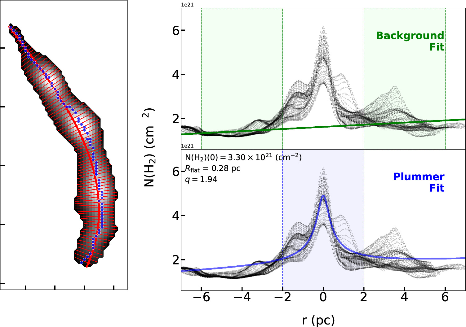
Figure A1. Musca. Left: column density map is used to build the radial profile of Musca by sampling radial cuts (red thin lines) with a step of 0.1 pc along the spine (thick red line). The spine is determined by Radfil using the provided mask using the B-spline smoothness algorithm (Zucker & Chen 2018). The radial distance is defined as the projected distance from the considered pixel to the peak emission (blue dot) on a given cut. Right: background fit (upper) and Plummer-like fit (lower). The results of the fit following Equation (10), are shown in the inserts. Green and blue shaded areas are the regions used for the background and Plummer-like fit, respectively.
Download figure:
Standard image High-resolution imageA.3. OMC-1
Figures A2 and A3 show in detail the comparison of our physical modeling results for P–Td and  , respectively, with the observational data for different regions in OMC-1, including north, south, BN-KL. The realistic polarization model with RAT-D best reproduces the observational data.
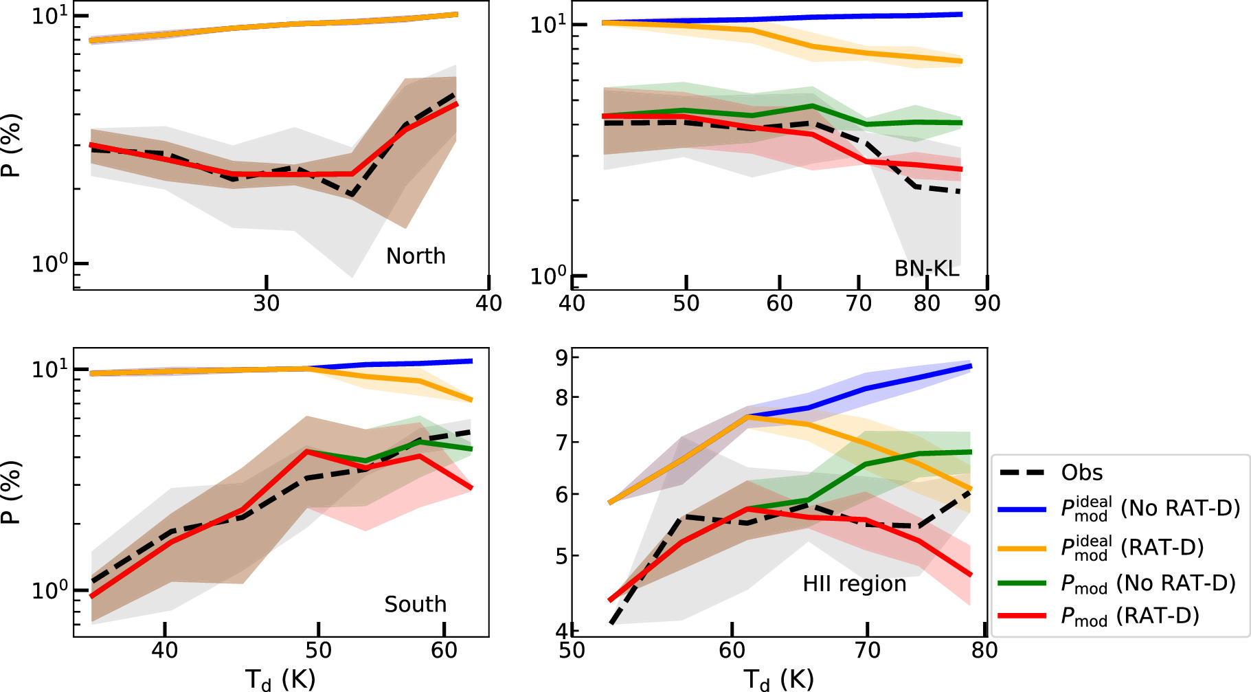
Figure A2. OMC-1. Comparison of the polarization degree vs. dust temperature relation from our models (color lines) with observational data (dashed line). The shaded area represents the 1σ deviation of each bin of data points.
Download figure:
Standard image High-resolution image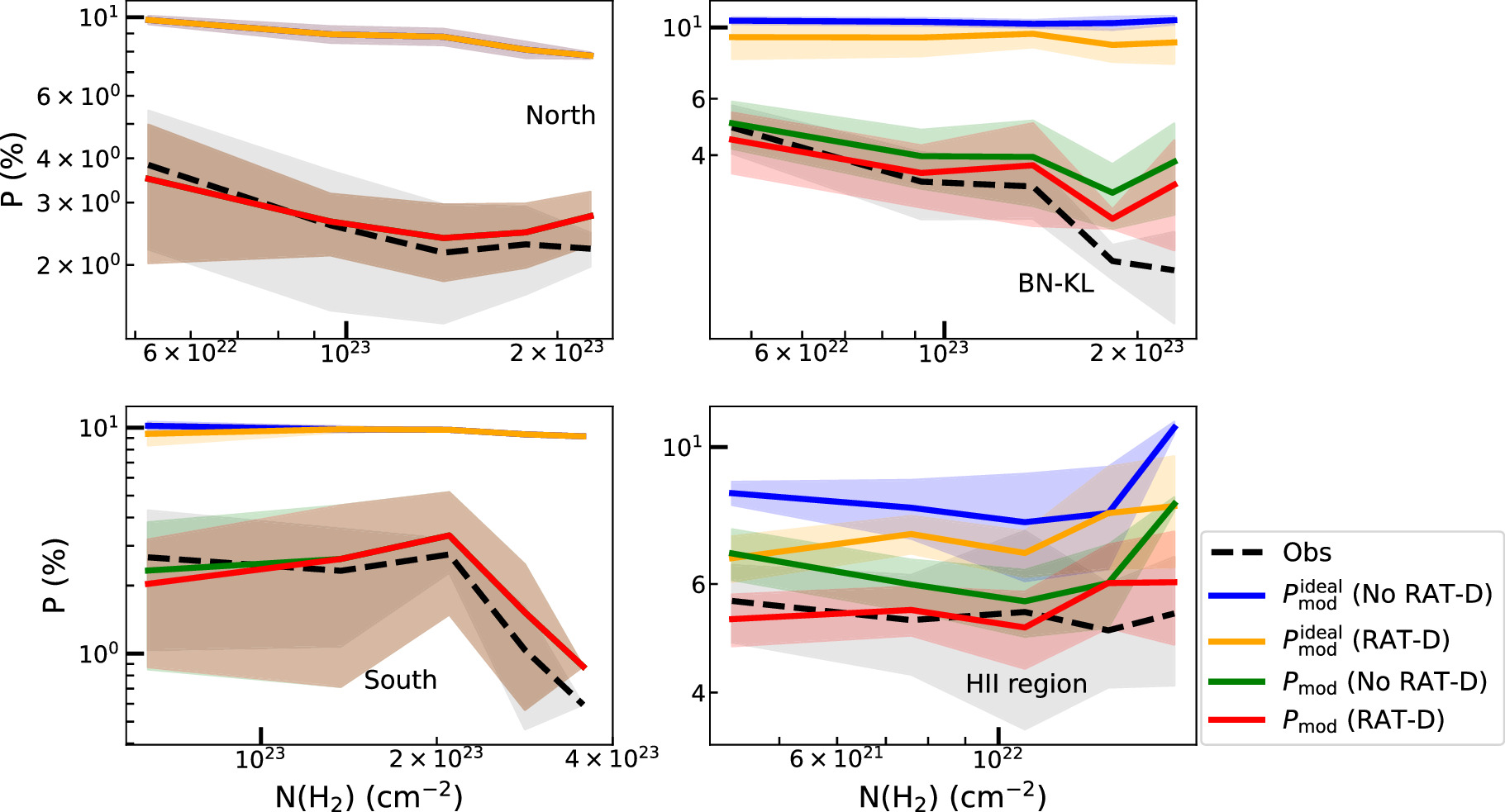
Figure A3. OMC-1. Comparison of the polarization degree vs. column density relation from our models (color lines) with observational data (dashed line). The shaded area represents the 1σ deviation of each bin of data points.
Download figure:
Standard image High-resolution imageFootnotes
- 6
- 7
Although ideal carbon grains being diamagnetic cannot be aligned with B-fields, hydrogenated carbon grains can be aligned with the B-fields because those grains contain unpaired electrons and become paramagnetic material (Hoang et al. 2023).