Abstract
We develop a two-dimensional B-spline approach in the cylindrical coordinate system to simulate spectra of lithium in magnetic fields of white dwarf stars. The advantage of the current approach is that it can be applied to calculate both low- and high-lying states, while the theoretical methods for describing magnetized lithium in the literature are limited to the treatment of the ground state and low-lying excited states. The magnetized atomic states are calculated with symmetries  ,
,  ,
,  ,
,  , and
, and  , and the lowest 10 atomic states of each symmetry are involved. The magnetic field strengths stride a scope of field strengths of white dwarf stars. Atomic data of absorption spectra corresponding to transitions from the ground state or low-lying excited states to high-lying excited states are reported for magnetized lithium. These atomic data include energy levels, wavelengths, and oscillator strengths. Comparison is made between our results, and theoretical and experimental data reported in the literature. The current two-dimensional B-spline approach can systematically produce atomic data to model discrete atomic spectra of both low- and high-lying states of lithium in magnetic white dwarf stars.
1. Introduction
Studies of atomic spectra in magnetic white dwarfs are of importance in astronomical application. One can determine the magnetic fields with the aid of discrete spectral lines, while information on the magnetic fields extracted from these spectra is crucial to understand the evolution of normal stars to magnetic white dwarfs (Ferrario et al. 2015). The study of properties of magnetic white dwarf stars shows that the magnetic fields should be taken into account in determining the initial–final mass relationship of stars, and also have an important influence on the outcomes of binary stellar evolution (Wickramasinghe & Ferrario 2000). In particular, it is found that the initial magnetic fields in stars increase with their evolution (Garstang 1977).
Besides the requirement in astronomical application, studies of atoms in a strong magnetic field are also of fundamental physical interest. In fact, magnetic white dwarfs offer physicists cosmic laboratories to test dynamical theories for describing strongly magnetized atoms and numerical algorithms for calculating their physical properties. The steady magnetic fields with such high strengths are unattainable in terrestrial laboratories, where only transient strong magnetic fields may be implemented with strengths comparable to those of magnetic white dwarf stars (Garstang 1977).
Ever since the first, GRW+70.8247, of the magnetic white dwarf stars was identified by Kemp et al. (1970), interest in studies of magnetic white dwarfs has been enhanced. So far, more than 600 white dwarfs have been classified as magnetic with the aid of spectroscopic analysis (Ferrario et al. 2015). However, the magnetic fields of only 40% of these stars are well determined due to the lack of theoretical data of magnetized atoms, based on the Data Releases 7 and 10 of the Sloan Digital Sky Survey (Kepler et al. 2013, 2015). Obviously, atomic structure data for various magnetized atoms in different atomic states are needed to interpret the features of the astronomically observed spectra of magnetic white dwarfs. Although a great amount of endeavors have been devoted to the description of various atoms in the past decades (e.g., Garstang 1977; Ferrario et al. 2015), theories and computations are still far from meeting the requirements for simulating the astronomically observed spectra.
A vital headway on the solution of the atomic hydrogen problem in an arbitrary magnetic field was implemented in the 1980s. Rösner et al. (1984) established a multiconfiguration Hartree–Fock approach to calculate atomic structures of hydrogen atoms in magnetic fields of white dwarfs and neutron stars, and energy levels of the 31 ground states and lowly excited states are presented. Shortly afterward, the same group presented wavelengths, dipole strengths, oscillator strengths, and transition rates relevant to these 31 atomic states of magnetized hydrogen atoms (Forster et al. 1984). With the aid of this research result, the spectral lines of GRW+70.8247 are interpreted as the stationary transitions between the different hydrogen atomic states, and the magnetic field strength of its atmosphere is substantiated to be 100–320 MG (Angel et al. 1985; Wickramasinghe & Ferrario 1988).
A great deal of spectral data of magnetized hydrogen atoms have been published, including energy levels, wavelengths, dipole strengths, and oscillator strengths for a large variety of transitions in magnetic fields of both white dwarfs and neutron stars using various approaches (e.g., Zhao & Stancil 2006, 2007; Baye et al. 2008a, 2008b; Zhao & Liu 2019). These approaches in the literature are in general limited to treat the ground states and low-lying excited states. Recently, Schimeczek & Wunner (2014a) developed a two-dimensional finite element approach to calculate several hydrogen spectral series in an arbitrary magnetic field. The distinct advantage of their approach is that it can be applied to calculations of both low- and high-lying excited states. Energy levels of the 300 atomic states including highly excited states are reported, and the dipole strengths are presented for transitions between these 300 atomic states. Their atomic data cover a wide scope of magnetic fields ranging from 0 to ∼5 × 10⁶ MG (Schimeczek & Wunner 2014b).
Contrary to the atomic hydrogen problem in a magnetic field, which is well depicted, spectral data with sufficiently good precision for magnetized multielectronic atoms are sparsely reported due to difficulties of effectively treating effects of electron correlation in atomic and molecular systems in the presence of a strong magnetic field. Recently, calculations of helium atoms in a magnetic field were implemented by Becken et al. (1999). This is a significant theoretical progress with emphasis on astronomical application in recent years, and can be regarded as one of benchmark calculations for treating effects of electron correlation in atomic and molecular systems in the presence of a strong magnetic field. With the aid of this result, spectral features in the magnetic white dwarf GD 229 were interpreted, and the magnetic fields were determined to be 300–700 MG (Jordan et al. 1998). This is the first high-field magnetic DB white dwarf identified. More recently, several relatively heavy elements in the atmosphere of the magnetic DZ white dwarf LHS 2534 were discovered (Reid et al. 2000). The spectral lines for magnetized Na i, Mg i, Ca i, and Ca ii were identified, and the magnetic field is found to be 1.92 MG.
The reliable determination of the distribution of magnetic fields on the surfaces of magnetic white dwarfs and neutron stars needs accurate knowledge of atomic structures of magnetized multielectronic atoms (Schmelcher & Cederbaum 1997), and thus it is inevitable to effectively treat electron correlation effects in atomic and molecular systems in the presence of a strong magnetic field. However, the description of most magnetized multielectronic atoms in the literature mainly relies on Hartree–Fock theory (e.g., Ivanov & Schmelcher 2000; Schimeczek & Wunner 2014c), and electron correlation effects are included only in a few theoretical approaches for calculating two- and three-electron systems, such as He, He−, Li, and Be+ (Becken et al. 1999; Guan & Li 2001; Al-Hujaj & Schmelcher 2004; Turbiner & Lopez Vieyra 2013; Salas et al. 2015). In particular, it was discovered that several stable states in He− exist in white dwarf strength magnetic fields, based on the variational calculation containing effects of electron correlation (Turbiner & Lopez Vieyra 2013). It can be expected from their results that spectral lines of magnetized He− may be able to be utilized to identify some magnetic white dwarfs in the future.
Recently, several theoretical methods were reported to study atomic structures and properties of lithium in the presence of a strong magnetic field (Guan & Li 2001; Al-Hujaj & Schmelcher 2004; Salas et al. 2015), in all of which electron correlation effects are included. In the more recent work, we presented energy levels and spectral lines of lithium in the presence of a magnetic field using our previous approach, in which wave functions are expanded by means of the B-spline basis and spherical harmonics, and a model potential is adopted (Zhao 2018). It should be pointed out that our previous finite-basis-set method can only calculate the ground state and low-lying excited states, and it is inappropriate for the high-lying excited states. This is because more and more angular momenta states have to be included as the energy level of an atomic state becomes higher and higher, and as a consequence the size of the Hamiltonian matrix to diagonalize becomes larger and larger. Furthermore, we would emphasize that the other methods published by Guan & Li (2001), Al-Hujaj & Schmelcher (2004), and Salas et al. (2015) are applicable only to the ground state and low-lying excited states.
The existing methods of magnetized Li atoms in the literature can only simulate spectral lines between low-lying atomic states, and are invalid for computing spectral lines relevant to highly excited states. Apparently, it is required to develop a new theoretical approach to simulate spectral lines for transitions to highly excited states of lithium in the magnetic white dwarf stars. The present work is performed in order to meet such a requirement.
In this paper, the two-dimensional B-spline approach in the cylindrical coordinate system, developed to understand atomic properties of lithium in highly excited states in the presence of a magnetic field, is outlined in Section 2. Energy levels, wavelengths, and oscillator strengths are presented for the transitions from low-lying initial states to highly excited final states. The involved field strengths stride a scope of field strengths of magnetic white dwarf stars. In this section, our results are also compared to experimental and theoretical data available in the literature. The application of the present approach in astronomy and astrophysics is discussed in Section 4. Finally, we summarize the current significant results and give conclusions in Section 5. We will utilize atomic units (au) throughout the paper, unless otherwise stated.
2. Approach
2.1. 2D B-spline Expansion of Wave Functions and the Generalized Eigenvalue Problem
McMillan (1971) introduced a model potential to study the atomic lithium problem. In this paper, this model potential is utilized. We assume the infinite nuclear mass, and neglect relativistic effects, such as spin–orbit coupling. In the cylindrical coordinate system, the Hamiltonian of lithium in the presence of a constant magnetic field with the direction along the positive z-axis is written in the form
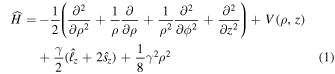
with

where  represents the model potential, given by McMillan (1971), with the two-dimensional boundary conditions

where the magnetic field strength γ is measured with B0 ≃ 2.35 × 10⁵ T,  and
and  are the z-component operators of the orbital and spin angular momentum of the outer valence electron, respectively, and the last two terms in Equation (1) represent the paramagnetic and diamagnetic potential. By setting α = β = 1.655, McMillan (1971) gives the model potential as specified in Equation (2). Here we modify this model potential by taking
  . We let β ≡ 1.6559, but take α = 1.6559 if
  , and α = 1.7848 if
  , where πz denotes the z-parity of the system, and m is the orbital magnetic quantum number. The reason to do such a modification is because the more exact energies of Li atomic states can be fitted based on those new parameters. We still use the notation of Becken et al. (1999),
  , to denote an atomic state of the Hamiltonian system, where m and sz denote the orbital and spin magnetic quantum number, s is the spin angular momentum quantum number, πz represents the z-parity of the system, and ν is the sequence number of the atomic state. The subscript sz is in general omissible as long as doing so does not cause confusion.
Following Schimeczek & Wunner (2014b), the wave function Ψ(ρ, z, ϕ) of the Hamiltonian (1) is expanded in the (ρ–z) plane in the B-spline basis  of order k,

where the order k of  is often omitted for simplification if no confusion is caused. Substituting Equation (4) into the two-dimensional Schrödinger equation for the Hamiltonian given by Equation (1) and projecting onto the basis
  yields the following matrix equation:

where H and  are the Hamiltonian and overlap matrices with matrix elements defined by


The presence of the overlap matrix  is due to application of the nonorthogonal B-spline basis functions. The resultant matrix Equation (5) is a generalized eigenvalue problem, and its solution is sketched out in the following subsection.
2.2. Computational Sketch
This subsection focuses on a brief overview of the numerical solution of the generalized eigenvalue problem (5). One of the most vital steps in the present calculations is to define knot sequences {ti} (i = 1, 2, 3, ……) in the limited regions of the ρ and z directions. The atomic system in low-lying electronic states in the presence of a weak magnetic field is more spherically symmetric, and hence it is very difficult to describe it in the cylindrical coordinate system. However, by suitably selecting the knot sequences and appropriately increasing the number of B-spline functions, it becomes feasible to optimize such more spherically symmetric states with a high precision in cylindrical coordinates. Let ρmax and zmax denote the maximum values of ρ and z, respectively. We distribute the respective knots {ti} in the intervals [0, ρmax] and [−zmax, zmax] with a linearly increasing spacing similar to that of Schimeczek & Wunner (2014a).
The routines of B-spline functions of de Boor (2001) are adopted to produce B-spline functions and their derivatives. The theory of B-spline functions is expatiated by de Boor (2001), and their application to calculations of magnetized atoms is outlined in Zhao & Stancil (2007). The details of B-spline functions and related applications can be found in these two references. The Hamiltonian and overlap matrix elements given in Equations (6) and (7) are calculated using Gaussian quadratures. The first and last functions of the B-spline basis set in the z direction are removed, and the last function of the B-spline basis set in the ρ direction is removed in order to enforce the physical boundary conditions. After obtaining all the Hamiltonian and overlap matrix elements, it is straightforward to solve this generalized eigenvalue problem, as done in Zhao (2018).  and zmax are optimally determined, and we increase the number of B-splines functions until the convergence of energies is obtained.
2.3. Spectral Line Calculations
Once the solution of the generalized eigenvalue problem (5) for the magnetized atomic states is implemented, their wave functions and energy levels are used to calculate spectral lines of the electric dipole transitions, including its wavelength, its dipole strength, and its oscillator strength. The dipole strength for the transition from an initial state Ψi to a final state Ψf is given by Engel et al. (2009)

where  denotes the dipole operator representing the interaction of radiation with atoms. The oscillator strength f for the dipole transition can be expressed in terms of the dipole strength dif,

where Ei and Ef denote the energy levels, corresponding to the atomic states Ψi and Ψf, respectively.
3. Results and Discussion
The current spectral calculations involve five symmetries  ,
,  ,
,  ,
,  , and
, and  for lithium in the presence of a magnetic field, and each symmetry contains the 10 lowest atomic states. Different from our previous work (Zhao 2018), which publishes spectra for the transitions to low-lying atomic states for lithium in the presence of a magnetic field, the current work focuses on reports of spectral lines for the transitions to highly excited states. All the field-free highly excited states are also calculated with the current two-dimensional B-spline approach in the cylindrical coordinates. In order to illustrate the correspondence of the current and traditional atomic state symbols, the correspondence examples of the two kinds of atomic state symbols are given in Table 1. One will see that this table is very convenient for comparison of the current spectral data with those from the National Institute of Standards and Technology (NIST) database in the field-free cases.
Table 1.
Correspondence of the Present,  , and Traditional Atomic State Symbols,
  where M Indicates the Total Orbital Magnetic Quantum Number and M = m, in Field-free Cases
| ν |

|

|

|

|

|
|---|---|---|---|---|---|
| 1 |

|

|

|

|

|
| 2 |

|

|

|

|

|
| 3 |

|

|

|

|

|
| 4 |

|

|

|

|

|
| 5 |

|

|

|

|

|
| 6 |

|

|

|

|

|
| 7 |

|

|

|

|

|
| 8 |

|

|

|

|

|
| 9 |

|

|

|

|

|
| 10 |

|

|

|

|

|
Note. The subscripts sz in  are omitted in the current work.
Download table as: ASCIITypeset image
Each of Tables 2–6 presents energy levels for the six highly excited states for one of the five symmetries as given above, as a function of magnetic fields γ ranging from 0 to 1 au. To our knowledge, no energy levels for these highly excited states of lithium in the presence of a magnetic field are reported, and hence no comparison is made for these highly excited states. However, the field-free energy levels of atomic lithium are available for these highly excited states. We perform comparison to the field-free experimental energy levels given in the NIST database in these tables. Our energy levels agree well with those from the NIST database for available atomic states.
Table 2.
Energy Levels in Atomic Units for the Highly Excited States ν  with ν = 5–10 as a Function of Magnetic Field Strengths γ
| γ (au) | 5 
|
6 
|
7 
|
8 
|
9 
|
10 
|
|---|---|---|---|---|---|---|
| 0.000 | −3.126046(−2) | −2.366913(−2) | −2.000607(−2) | −2.000000(−2) | −1.596393(−2) | −1.389263(−2) |
| ⋯ | −3.127342(−2) | −2.363651(−2) | −2.001223(−2) | ⋯ | −1.594478(−2) | −1.389590(−2) |
| 0.001 | −3.173053(−2) | −2.407604(−2) | −2.046416(−2) | −2.041133(−2) | −1.626417(−2) | −1.430622(−2) |
| 0.002 | −3.214133(−2) | −2.430611(−2) | −2.085240(−2) | −2.063774(−2) | −1.623065(−2) | −1.455567(−2) |
| 0.003 | −3.249440(−2) | −2.438507(−2) | −2.116699(−2) | −2.069687(−2) | −1.603086(−2) | −1.461614(−2) |
| 0.004 | −3.279182(−2) | −2.435022(−2) | −2.140612(−2) | −2.060304(−2) | −1.585906(−2) | −1.443244(−2) |
| 0.005 | −3.303578(−2) | −2.424530(−2) | −2.156447(−2) | −2.036899(−2) | −1.579019(−2) | −1.402127(−2) |
| 0.006 | −3.322821(−2) | −2.411512(−2) | −2.163365(−2) | −2.000781(−2) | −1.577038(−2) | −1.348074(−2) |
| 0.007 | −3.337056(−2) | −2.399799(−2) | −2.160605(−2) | −1.953775(−2) | −1.574485(−2) | −1.288017(−2) |
| 0.008 | −3.346376(−2) | −2.391673(−2) | −2.148167(−2) | −1.898858(−2) | −1.567760(−2) | −1.225268(−2) |
| 0.009 | −3.350823(−2) | −2.387519(−2) | −2.127169(−2) | −1.840921(−2) | −1.553093(−2) | −1.175191(−2) |
| 0.010 | −3.350400(−2) | −2.386457(−2) | −2.099385(−2) | −1.787173(−2) | −1.525451(−2) | −1.168941(−2) |
| 0.020 | −3.089629(−2) | −2.390925(−2) | −1.699116(−2) | −1.616451(−2) | −1.215385(−2) | −9.270458(−3) |
| 0.030 | −2.661403(−2) | −2.204154(−2) | −1.653396(−2) | −1.208624(−2) | −9.848369(−3) | −8.979685(−3) |
| 0.040 | −2.576004(−2) | −1.784334(−2) | −1.440861(−2) | −1.170443(−2) | −8.996102(−3) | −7.043312(−3) |
| 0.050 | −2.582237(−2) | −1.738282(−2) | −1.249182(−2) | −9.445100(−3) | −7.474974(−3) | −6.209006(−3) |
| 0.060 | −2.600796(−2) | −1.740791(−2) | −1.243059(−2) | −9.307725(−3) | −7.224867(−3) | −5.768214(−3) |
| 0.070 | −2.621378(−2) | −1.749004(−2) | −1.246251(−2) | −9.317195(−3) | −7.223767(−3) | −5.762125(−3) |
| 0.080 | −2.641489(−2) | −1.758236(−2) | −1.251001(−2) | −9.343804(−3) | −7.239697(−3) | −5.772183(−3) |
| 0.090 | −2.660376(−2) | −1.767309(−2) | −1.255954(−2) | −9.373513(−3) | −7.258825(−3) | −5.785192(−3) |
| 0.100 | −2.677831(−2) | −1.775830(−2) | −1.260702(−2) | −9.402591(−3) | −7.277904(−3) | −5.798386(−3) |
| 0.200 | −1.834419(−2) | −1.295230(−2) | −9.623354(−3) | −7.427659(−3) | −5.904653(−3) | −4.805607(−3) |
| 0.300 | −1.857145(−2) | −1.308032(−2) | −9.701942(−3) | −7.479163(−3) | −5.940172(−3) | −4.831117(−3) |
| 0.400 | −1.862757(−2) | −1.311112(−2) | −9.720586(−3) | −7.491295(−3) | −5.948510(−3) | −4.837098(−3) |
| 0.500 | −1.858054(−2) | −1.308186(−2) | −9.701302(−3) | −7.477970(−3) | −5.938943(−3) | −4.830009(−3) |
| 0.600 | −1.846982(−2) | −1.301509(−2) | −9.658119(−3) | −7.448503(−3) | −5.917967(−3) | −4.814560(−3) |
| 0.700 | −1.832342(−2) | −1.292698(−2) | −9.601198(−3) | −7.409686(−3) | −5.890346(−3) | −4.794224(−3) |
| 0.800 | −1.816270(−2) | −1.283005(−2) | −9.538486(−3) | −7.366870(−3) | −5.859852(−3) | −4.771752(−3) |
| 0.900 | −1.800320(−2) | −1.273357(−2) | −9.475933(−3) | −7.324095(−3) | −5.829349(−3) | −4.749255(−3) |
| 1.000 | −1.785485(−2) | −1.264358(−2) | −9.417463(−3) | −7.284048(−3) | −5.800757(−3) | −4.728144(−3) |
Note. The field-free energy levels are compared to the experimental values from the NIST database: http://physics.nist.gov. The NIST results and ours are listed in the low and upper rows for the field-free cases, respectively.
Download table as: ASCIITypeset image
Table 3.
Same as Table 2, but for the Highly Excited States ν  with ν = 5–10
| γ (au) | 5 
|
6 
|
7 
|
8 
|
9 
|
10 
|
|---|---|---|---|---|---|---|
| 0.000 | −2.039437(−2) | −2.000004(−2) | −1.411852(−2) | −1.388892(−2) | −1.388889(−2) | −1.034917(−2) |
| ⋯ | −2.037390(−2) | −1.996867(−2) | −1.410766(−2) | ⋯ | ⋯ | −1.034181(−2) |
| 0.001 | −2.125411(−2) | −2.092273(−2) | −1.485945(−2) | −1.479129(−2) | −1.467244(−2) | −1.105580(−2) |
| 0.002 | −2.190470(−2) | −2.163599(−2) | −1.557958(−2) | −1.531762(−2) | −1.481142(−2) | −1.162839(−2) |
| 0.003 | −2.253991(−2) | −2.198838(−2) | −1.620341(−2) | −1.563129(−2) | −1.443922(−2) | −1.202353(−2) |
| 0.004 | −2.313354(−2) | −2.205955(−2) | −1.671017(−2) | −1.579292(−2) | −1.373181(−2) | −1.229827(−2) |
| 0.005 | −2.365857(−2) | −2.192986(−2) | −1.711778(−2) | −1.585117(−2) | −1.279950(−2) | −1.248499(−2) |
| 0.006 | −2.412186(−2) | −2.164055(−2) | −1.744254(−2) | −1.584087(−2) | −1.260348(−2) | −1.174686(−2) |
| 0.007 | −2.453357(−2) | −2.122321(−2) | −1.769857(−2) | −1.578361(−2) | −1.266776(−2) | −1.074174(−2) |
| 0.008 | −2.490279(−2) | −2.070522(−2) | −1.789769(−2) | −1.569047(−2) | −1.269035(−2) | −1.017800(−2) |
| 0.009 | −2.523687(−2) | −2.011309(−2) | −1.804828(−2) | −1.556519(−2) | −1.268115(−2) | −1.001754(−2) |
| 0.010 | −2.554147(−2) | −1.947967(−2) | −1.814964(−2) | −1.540732(−2) | −1.264628(−2) | −9.927710(−3) |
| 0.020 | −2.748055(−2) | −1.900644(−2) | −1.388953(−2) | −1.300707(−2) | −1.049689(−2) | −8.402651(−3) |
| 0.030 | −2.706746(−2) | −1.938928(−2) | −1.392032(−2) | −1.037862(−2) | −8.009396(−3) | −6.853838(−3) |
| 0.040 | −2.430731(−2) | −1.874984(−2) | −1.386576(−2) | −1.038950(−2) | −8.012177(−3) | −6.346956(−3) |
| 0.050 | −2.295569(−2) | −1.681555(−2) | −1.291651(−2) | −1.001672(−2) | −7.851063(−3) | −6.266681(−3) |
| 0.060 | −2.283009(−2) | −1.605099(−2) | −1.187372(−2) | −9.132539(−3) | −7.230798(−3) | −5.852056(−3) |
| 0.070 | −2.295857(−2) | −1.595378(−2) | −1.165402(−2) | −8.857960(−3) | −6.947341(−3) | −5.587785(−3) |
| 0.080 | −2.311317(−2) | −1.599076(−2) | −1.163478(−2) | −8.816025(−3) | −6.898800(−3) | −5.539952(−3) |
| 0.090 | −2.323223(−2) | −1.604904(−2) | −1.165726(−2) | −8.821549(−3) | −6.896813(−3) | −5.534924(−3) |
| 0.100 | −2.328750(−2) | −1.609529(−2) | −1.168403(−2) | −8.836439(−3) | −6.905175(−3) | −5.539701(−3) |
| 0.200 | −1.930463(−2) | −1.371869(−2) | −1.022040(−2) | −7.890544(−3) | −6.265085(−3) | −5.088764(−3) |
| 0.300 | −1.905979(−2) | −1.338499(−2) | −9.903490(−3) | −7.618842(−3) | −6.040691(−3) | −4.905734(−3) |
| 0.400 | −1.937036(−2) | −1.355042(−2) | −1.000125(−2) | −7.681228(−3) | −6.082904(−3) | −4.935629(−3) |
| 0.500 | −1.967389(−2) | −1.372143(−2) | −1.010696(−2) | −7.751135(−3) | −6.131544(−3) | −4.970844(−3) |
| 0.600 | −1.994061(−2) | −1.387297(−2) | −1.020122(−2) | −7.813737(−3) | −6.175241(−3) | −5.002554(−3) |
| 0.700 | −2.017392(−2) | −1.400574(−2) | −1.028389(−2) | −7.868686(−3) | −6.213612(−3) | −5.030407(−3) |
| 0.800 | −2.037993(−2) | −1.412296(−2) | −1.035686(−2) | −7.917175(−3) | −6.247465(−3) | −5.054974(−3) |
| 0.900 | −2.056385(−2) | −1.422751(−2) | −1.042191(−2) | −7.960379(−3) | −6.277615(−3) | −5.076846(−3) |
| 1.000 | −2.072971(−2) | −1.432170(−2) | −1.048047(−2) | −7.999246(−3) | −6.304725(−3) | −5.096505(−3) |
Download table as: ASCIITypeset image
Table 4.
Same as Table 2, but for the Highly Excited States ν with ν = 5–10
| γ (au) | 5 
|
6 
|
7 
|
8 
|
9 
|
10 
|
|---|---|---|---|---|---|---|
| 0.000 | −1.389263(−2) | −1.388889(−2) | −1.020653(−2) | −1.020408(−2) | −1.020408(−2) | −7.814175(−3) |
| ⋯ | −1.389590(−2) | ⋯ | −1.020897(−2) | ⋯ | ⋯ | −7.817821(−3) |
| 0.001 | −1.524046(−2) | −1.507353(−2) | −1.153125(−2) | −1.138454(−2) | −1.110802(−2) | −8.995107(−3) |
| 0.002 | −1.632060(−2) | −1.568325(−2) | −1.254585(−2) | −1.205158(−2) | −1.105702(−2) | −9.706198(−3) |
| 0.003 | −1.718674(−2) | −1.585629(−2) | −1.331142(−2) | −1.241543(−2) | −1.043720(−2) | −1.014291(−2) |
| 0.004 | −1.789545(−2) | −1.571884(−2) | −1.388276(−2) | −1.262107(−2) | −1.040818(−2) | −9.559214(−3) |
| 0.005 | −1.848993(−2) | −1.537539(−2) | −1.429834(−2) | −1.274068(−2) | −1.053249(−2) | −8.988411(−3) |
| 0.006 | −1.899952(−2) | −1.495164(−2) | −1.455552(−2) | −1.278766(−2) | −1.056546(−2) | −8.855990(−3) |
| 0.007 | −1.944253(−2) | −1.490068(−2) | −1.433010(−2) | −1.272725(−2) | −1.054117(−2) | −8.742467(−3) |
| 0.008 | −1.982911(−2) | −1.504234(−2) | −1.394223(−2) | −1.250379(−2) | −1.046849(−2) | −8.591076(−3) |
| 0.009 | −2.016338(−2) | −1.516713(−2) | −1.366775(−2) | −1.215064(−2) | −1.031883(−2) | −8.431078(−3) |
| 0.010 | −2.044471(−2) | −1.527886(−2) | −1.345150(−2) | −1.182838(−2) | −1.005054(−2) | −8.281276(−3) |
| 0.020 | −1.963020(−2) | −1.594898(−2) | −1.203179(−2) | −9.267198(−3) | −8.775359(−3) | −7.206995(−3) |
| 0.030 | −1.868602(−2) | −1.397079(−2) | −1.132721(−2) | −9.161485(−3) | −7.286922(−3) | −5.864613(−3) |
| 0.040 | −1.924774(−2) | −1.376978(−2) | −1.030732(−2) | −8.010886(−3) | −6.424102(−3) | −5.288059(−3) |
| 0.050 | −1.981125(−2) | −1.403955(−2) | −1.040536(−2) | −7.998752(−3) | −6.331240(−3) | −5.131433(−3) |
| 0.060 | −2.025264(−2) | −1.430068(−2) | −1.055683(−2) | −8.089118(−3) | −6.386642(−3) | −5.166127(−3) |
| 0.070 | −2.051476(−2) | −1.450983(−2) | −1.069084(−2) | −8.176541(−3) | −6.445914(−3) | −5.207842(−3) |
| 0.080 | −2.041572(−2) | −1.463950(−2) | −1.079292(−2) | −8.248001(−3) | −6.496365(−3) | −5.244395(−3) |
| 0.090 | −1.940370(−2) | −1.460060(−2) | −1.084135(−2) | −8.294231(−3) | −6.532517(−3) | −5.271939(−3) |
| 0.100 | −1.746060(−2) | −1.399729(−2) | −1.074870(−2) | −8.286836(−3) | −6.541650(−3) | −5.283537(−3) |
| 0.200 | −1.679404(−2) | −1.203507(−2) | −9.036430(−3) | −7.029625(−3) | −5.622367(−3) | −4.598180(−3) |
| 0.300 | −1.748853(−2) | −1.244277(−2) | −9.295638(−3) | −7.204529(−3) | −5.745928(−3) | −4.688703(−3) |
| 0.400 | −1.798709(−2) | −1.273532(−2) | −9.481695(−3) | −7.330127(−3) | −5.834688(−3) | −4.753745(−3) |
| 0.500 | −1.837117(−2) | −1.295983(−2) | −9.624102(−3) | −7.426071(−3) | −5.902387(−3) | −4.803292(−3) |
| 0.600 | −1.868237(−2) | −1.314110(−2) | −9.738805(−3) | −7.503211(−3) | −5.956741(−3) | −4.843027(−3) |
| 0.700 | −1.894354(−2) | −1.329278(−2) | −9.834581(−3) | −7.567522(−3) | −6.002001(−3) | −4.876082(−3) |
| 0.800 | −1.916839(−2) | −1.342303(−2) | −9.916683(−3) | −7.622579(−3) | −6.040708(−3) | −4.904327(−3) |
| 0.900 | −1.936576(−2) | −1.353711(−2) | −9.988482(−3) | −7.670670(−3) | −6.074487(−3) | −4.928958(−3) |
| 1.000 | −1.954166(−2) | −1.363858(−2) | −1.005225(−2) | −7.713342(−3) | −6.104436(−3) | −4.950782(−3) |
Download table as: ASCIITypeset image
Table 5.
Same as Table 2, but for the Highly Excited States ν  with ν = 5–10
| γ (au) | 5 
|
6 
|
7 
|
8 
|
9 
|
10 
|
|---|---|---|---|---|---|---|
| 0.000 | −2.039437(−2) | −2.000004(−2) | −1.411852(−2) | −1.388892(−2) | −1.388889(−2) | −1.034917(−2) |
| ⋯ | −2.037390(−2) | −1.996867(−2) | −1.410766(−2) | ⋯ | ⋯ | −1.034181(−2) |
| 0.001 | −2.082633(−2) | −2.042824(−2) | −1.449711(−2) | −1.430326(−2) | −1.418973(−2) | −1.068836(−2) |
| 0.002 | −2.116288(−2) | −2.068267(−2) | −1.479578(−2) | −1.450627(−2) | −1.404165(−2) | −1.094482(−2) |
| 0.003 | −2.146411(−2) | −2.073062(−2) | −1.505667(−2) | −1.451704(−2) | −1.354063(−2) | −1.111887(−2) |
| 0.004 | −2.173857(−2) | −2.059908(−2) | −1.526305(−2) | −1.438740(−2) | −1.281096(−2) | −1.123326(−2) |
| 0.005 | −2.198192(−2) | −2.032882(−2) | −1.542212(−2) | −1.414907(−2) | −1.194703(−2) | −1.130504(−2) |
| 0.006 | −2.219534(−2) | −1.995221(−2) | −1.554400(−2) | −1.382358(−2) | −1.135994(−2) | −1.100673(−2) |
| 0.007 | −2.238239(−2) | −1.949514(−2) | −1.563675(−2) | −1.342848(−2) | −1.137149(−2) | −1.007657(−2) |
| 0.008 | −2.254679(−2) | −1.897959(−2) | −1.570530(−2) | −1.298421(−2) | −1.135519(−2) | −9.171621(−3) |
| 0.009 | −2.269172(−2) | −1.842580(−2) | −1.575060(−2) | −1.252797(−2) | −1.128180(−2) | −8.736864(−3) |
| 0.010 | −2.281974(−2) | −1.785580(−2) | −1.576732(−2) | −1.214000(−2) | −1.108279(−2) | −8.716347(−3) |
| 0.020 | −2.343398(−2) | −1.633044(−2) | −1.217238(−2) | −1.053828(−2) | −8.781387(−3) | −6.972367(−3) |
| 0.030 | −2.299343(−2) | −1.623284(−2) | −1.187220(−2) | −9.031496(−3) | −7.099472(−3) | −5.736534(−3) |
| 0.040 | −2.136349(−2) | −1.581330(−2) | −1.165160(−2) | −8.866381(−3) | −6.951596(−3) | −5.587810(−3) |
| 0.050 | −1.933355(−2) | −1.496724(−2) | −1.128767(−2) | −8.656435(−3) | −6.810827(−3) | −5.485674(−3) |
| 0.060 | −1.796826(−2) | −1.374738(−2) | −1.068204(−2) | −8.341398(−3) | −6.621762(−3) | −5.360140(−3) |
| 0.070 | −1.728575(−2) | −1.279750(−2) | −9.889565(−3) | −7.833767(−3) | −6.308828(−3) | −5.158796(−3) |
| 0.080 | −1.693996(−2) | −1.233596(−2) | −9.382813(−3) | −7.371076(−3) | −5.935470(−3) | −4.874005(−3) |
| 0.090 | −1.675057(−2) | −1.211733(−2) | −9.157896(−3) | −7.155777(−3) | −5.739853(−3) | −4.702634(−3) |
| 0.100 | −1.664324(−2) | −1.200320(−2) | −9.050233(−3) | −7.059433(−3) | −5.655945(−3) | −4.630588(−3) |
| 0.200 | −1.666215(−2) | −1.193668(−2) | −8.964628(−3) | −6.976700(−3) | −5.582642(−3) | −4.567779(−3) |
| 0.300 | −1.693180(−2) | −1.209158(−2) | −9.061715(−3) | −7.041576(−3) | −5.628162(−3) | −4.600964(−3) |
| 0.400 | −1.716905(−2) | −1.223122(−2) | −9.150817(−3) | −7.101907(−3) | −5.670913(−3) | −4.632366(−3) |
| 0.500 | −1.736904(−2) | −1.234942(−2) | −9.226441(−3) | −7.153210(−3) | −5.707313(−3) | −4.659127(−3) |
| 0.600 | −1.753995(−2) | −1.245049(−2) | −9.291129(−3) | −7.197098(−3) | −5.738454(−3) | −4.682021(−3) |
| 0.700 | −1.768867(−2) | −1.253840(−2) | −9.347377(−3) | −7.235248(−3) | −5.765515(−3) | −4.701909(−3) |
| 0.800 | −1.782017(−2) | −1.261608(−2) | −9.397045(−3) | −7.268917(−3) | −5.789388(−3) | −4.719449(−3) |
| 0.900 | −1.793800(−2) | −1.268562(−2) | −9.441478(−3) | −7.299023(−3) | −5.810724(−3) | −4.735119(−3) |
| 1.000 | −1.804473(−2) | −1.274855(−2) | −9.481665(−3) | −7.326237(−3) | −5.830003(−3) | −4.749273(−3) |
Download table as: ASCIITypeset image
Table 6.
Same as Table 2, but for the Highly Excited States ν with ν = 5–10
| γ (au) | 5 
|
6 
|
7 
|
8 
|
9 
|
10 
|
|---|---|---|---|---|---|---|
| 0.000 | −1.389263(−2) | −1.388889(−2) | −1.020653(−2) | −1.020408(−2) | −1.020408(−2) | −7.814175(−3) |
| ⋯ | −1.389590(−2) | ⋯ | −1.020897(−2) | ⋯ | ⋯ | −7.817821(−3) |
| 0.001 | −1.478593(−2) | −1.465142(−2) | −1.106726(−2) | −1.096403(−2) | −1.073774(−2) | −8.583849(−3) |
| 0.002 | −1.549139(−2) | −1.498158(−2) | −1.168141(−2) | −1.132884(−2) | −1.053435(−2) | −9.011494(−3) |
| 0.003 | −1.604465(−2) | −1.499002(−2) | −1.209936(−2) | −1.144299(−2) | −9.930504(−3) | −9.236852(−3) |
| 0.004 | −1.648410(−2) | −1.478356(−2) | −1.237210(−2) | −1.139934(−2) | −9.422770(−3) | −9.095820(−3) |
| 0.005 | −1.683867(−2) | −1.445246(−2) | −1.253609(−2) | −1.124334(−2) | −9.431160(−3) | −8.382231(−3) |
| 0.006 | −1.712736(−2) | −1.407932(−2) | −1.260201(−2) | −1.100461(−2) | −9.407816(−3) | −7.716601(−3) |
| 0.007 | −1.736182(−2) | −1.375664(−2) | −1.254055(−2) | −1.072463(−2) | −9.314603(−3) | −7.514965(−3) |
| 0.008 | −1.754887(−2) | −1.356875(−2) | −1.230708(−2) | −1.046404(−2) | −9.121085(−3) | −7.456478(−3) |
| 0.009 | −1.769254(−2) | −1.350613(−2) | −1.193716(−2) | −1.026449(−2) | −8.829597(−3) | −7.360408(−3) |
| 0.010 | −1.779542(−2) | −1.350332(−2) | −1.152193(−2) | −1.010434(−2) | −8.514909(−3) | −7.196409(−3) |
| 0.020 | −1.736607(−2) | −1.324787(−2) | −1.030690(−2) | −8.194238(−3) | −6.653613(−3) | −5.517220(−3) |
| 0.030 | −1.687067(−2) | −1.262516(−2) | −9.664766(−3) | −7.607276(−3) | −6.133420(−3) | −5.043444(−3) |
| 0.040 | −1.637726(−2) | −1.242802(−2) | −9.475195(−3) | −7.402662(−3) | −5.924308(−3) | −4.840831(−3) |
| 0.050 | −1.513790(−2) | −1.196489(−2) | −9.325234(−3) | −7.330803(−3) | −5.876821(−3) | −4.803992(−3) |
| 0.060 | −1.416946(−2) | −1.085710(−2) | −8.676711(−3) | −7.030561(−3) | −5.732068(−3) | −4.725381(−3) |
| 0.070 | −1.394318(−2) | −1.038402(−2) | −8.040417(−3) | −6.416932(−3) | −5.244263(−3) | −4.366692(−3) |
| 0.080 | −1.394472(−2) | −1.031343(−2) | −7.927279(−3) | −6.278355(−3) | −5.092594(−3) | −4.212018(−3) |
| 0.090 | −1.400818(−2) | −1.033031(−2) | −7.922467(−3) | −6.263685(−3) | −5.073960(−3) | −4.192406(−3) |
| 0.100 | −1.409049(−2) | −1.037164(−2) | −7.943841(−3) | −6.274819(−3) | −5.079642(−3) | −4.195111(−3) |
| 0.200 | −1.483650(−2) | −1.081712(−2) | −8.229840(−3) | −6.468940(−3) | −5.217308(−3) | −4.296244(−3) |
| 0.300 | −1.531574(−2) | −1.110910(−2) | −8.420729(−3) | −6.600551(−3) | −5.311879(−3) | −4.366485(−3) |
| 0.400 | −1.565509(−2) | −1.131531(−2) | −8.555307(−3) | −6.693206(−3) | −5.378380(−3) | −4.415829(−3) |
| 0.500 | −1.591562(−2) | −1.147319(−2) | −8.658125(−3) | −6.763883(−3) | −5.429043(−3) | −4.453381(−3) |
| 0.600 | −1.612628(−2) | −1.160053(−2) | −8.740916(−3) | −6.820718(−3) | −5.469739(−3) | −4.483518(−3) |
| 0.700 | −1.630279(−2) | −1.170701(−2) | −8.810041(−3) | −6.868115(−3) | −5.503647(−3) | −4.508610(−3) |
| 0.800 | −1.645456(−2) | −1.179841(−2) | −8.869295(−3) | −6.908704(−3) | −5.532661(−3) | −4.530067(−3) |
| 0.900 | −1.658764(−2) | −1.187843(−2) | −8.921112(−3) | −6.944168(−3) | −5.557994(−3) | −4.548790(−3) |
| 1.000 | −1.670613(−2) | −1.194957(−2) | −8.967138(−3) | −6.975644(−3) | −5.580464(−3) | −4.565389(−3) |
Download table as: ASCIITypeset image
Although no energy levels of highly excited states of magnetized Li atoms are published, their atomic structures of the low-lying states have been studied. Here we perform calculations of the low-lying atomic states of Li in magnetic fields to check the current two-dimensional B-spline approach by comparing with these published data. Energy levels of the lowest four atomic states for each of these five symmetries, as given in Tables 2–6, are obtained with a scope of magnetic field strengths γ from 0.001 to 1 au. We noticed that seven significant digits of energy levels for each atomic state from the current two-dimensional B-spline approach and our previous theoretical approach (Zhao 2018) are consistent without exception in this scope of magnetic fields. Figure 1 illustrates the current ionization energies for the selected atomic states. The two symmetries  and
and  are illustrated, and the lowest four atomic states are contained for each symmetry. Our previous ionization energies (Zhao 2018) are also plotted in this figure to show such a contrast.
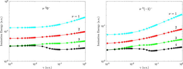
Figure 1. Comparison of ionization energies for the atomic states  and
and  with ν = 1–4 from the current two-dimensional B-spline approach and from our previous theoretical approach (Zhao 2018) as a function of magnetic field strengths γ. The filled and open dots represent the current calculations and those of Zhao (2018), respectively. Note: the dots are connected with a solid line as a visual guide.
Download figure:
Standard image High-resolution imageSince detailed comparison of our ionization energies of the low-lying atomic states to those from the other methods has been made for the other three symmetries  ,
,  , and
, and  in Zhao (2018), a similar discussion with the help of a diagram is distinctly dispensable for these three symmetries. Details of this discussion should be found in Zhao (2018), where our results were found to be in good agreement with the data of Al-Hujaj & Schmelcher (2004) for the low-lying three atomic states, but the discrepancies become remarkable for the states with ν = 4. The reasons that cause such discrepancies have been analyzed in Zhao (2018), and hence are omitted here.
It is well known that in the weak-field cases, Li atomic systems in the low-lying atomic states are more spherically symmetric. For such systems, our previous approach in the spherical coordinate (Zhao 2018) should be more valid. In the current calculations for all these weak-field atomic states, however, the two-dimensional B-spline approach in the cylindrical coordinate can also produce the ionization energies exact enough. Considering the difficulty using the cylindrical coordinate to describe the atomic systems with highly spherical symmetry, our current theoretical approach is fabulous. Such good results may be attributed to one of the powerful properties of B-spline functions (see de Boor 2001 for details). The powerful property is that B-spline functions permit one to flexibly select the knot sequences according to the distribution of wave functions.
The spectral lines are calculated for the transitions to highly excited states from the three low-lying states  ,
,  , and
, and  . A total of 30 transitions are included. The wavelengths and oscillator strengths corresponding to these transitions are presented with a scope of magnetic field strengths γ from 0.001 to 1 au in Tables 7–11. As no spectral data as given in Tables 7–11 are reported in the literature, it is impossible to perform any comparison for these spectral lines. In order to check the reliability of the current two-dimensional B-spline approach in the calculations of spectral lines, the wavelengths and oscillator strengths for the transitions to low-lying atomic states from
  and
and  are calculated with the current two-dimensional B-spline approach, and comparison is made to available data.
Table 7.
Wavelengths λ and Oscillator Strengths f for the Transitions 1  with ν = 5–10 as a Function of Magnetic Field Strengths γ
| γ (au) | ν = 5 | 6 | 7 | 8 | 9 | 10 | ||||||
|---|---|---|---|---|---|---|---|---|---|---|---|---|
| λ(Å) | f | λ(Å) | f | λ(Å) | f | λ(Å) | f | λ(Å) | f | λ(Å) | f | |
| 0.001 | 2568.6 | 2.549(−3) | 2563.8 | 2.197(−5) | 2479.2 | 1.142(−3) | 2478.3 | 2.133(−4) | 2476.7 | 2.674(−4) | 2429.0 | 1.188(−4) |
| 0.002 | 2570.8 | 1.961(−3) | 2567.0 | 7.154(−4) | 2482.3 | 9.670(−5) | 2478.7 | 4.568(−4) | 2471.9 | 1.241(−3) | 2430.0 | 7.366(−5) |
| 0.003 | 2572.9 | 9.207(−4) | 2564.9 | 1.918(−3) | 2484.0 | 7.880(−5) | 2476.3 | 3.753(−4) | 2460.4 | 1.560(−3) | 2428.7 | 8.753(−5) |
| 0.004 | 2574.4 | 6.532(−4) | 2558.9 | 2.386(−3) | 2484.3 | 8.860(−5) | 2471.9 | 3.719(−4) | 2444.6 | 1.774(−3) | 2425.9 | 1.137(−4) |
| 0.005 | 2575.0 | 5.832(−4) | 2550.1 | 2.676(−3) | 2483.2 | 1.098(−4) | 2466.2 | 3.864(−4) | 2426.1 | 1.917(−3) | 2422.0 | 1.372(−4) |
| 0.006 | 2574.7 | 5.724(−4) | 2539.1 | 2.910(−3) | 2481.0 | 1.423(−4) | 2459.6 | 4.055(−4) | 2417.3 | 2.209(−4) | 2406.4 | 1.854(−3) |
| 0.007 | 2573.7 | 5.881(−4) | 2526.4 | 3.106(−3) | 2478.0 | 1.904(−4) | 2452.5 | 4.250(−4) | 2412.0 | 2.834(−4) | 2387.7 | 1.449(−3) |
| 0.008 | 2572.1 | 6.195(−4) | 2512.5 | 3.248(−3) | 2474.2 | 2.649(−4) | 2444.9 | 4.448(−4) | 2406.2 | 3.635(−4) | 2374.7 | 5.474(−4) |
| 0.009 | 2570.0 | 6.627(−4) | 2497.8 | 3.298(−3) | 2469.9 | 3.957(−4) | 2437.1 | 4.667(−4) | 2400.1 | 4.597(−4) | 2366.8 | 3.155(−4) |
| 0.010 | 2567.6 | 7.163(−4) | 2482.8 | 3.127(−3) | 2464.9 | 6.945(−4) | 2428.9 | 4.932(−4) | 2393.7 | 5.757(−4) | 2360.0 | 3.200(−4) |
| 0.020 | 2530.1 | 2.123(−3) | 2416.4 | 3.695(−4) | 2352.6 | 2.601(−4) | 2341.9 | 1.632(−3) | 2312.1 | 2.917(−4) | 2287.7 | 8.574(−4) |
| 0.030 | 2465.8 | 7.112(−3) | 2367.4 | 1.405(−3) | 2302.0 | 3.858(−4) | 2261.5 | 1.473(−4) | 2235.2 | 1.100(−4) | 2222.6 | 2.140(−3) |
| 0.040 | 2378.5 | 7.315(−3) | 2311.5 | 5.178(−3) | 2255.6 | 1.549(−3) | 2217.4 | 5.663(−4) | 2192.1 | 2.559(−4) | 2174.6 | 1.331(−4) |
| 0.050 | 2316.8 | 2.233(−3) | 2246.6 | 5.005(−3) | 2204.3 | 4.652(−3) | 2173.8 | 2.486(−3) | 2151.5 | 1.218(−3) | 2135.6 | 6.504(−4) |
| 0.060 | 2274.8 | 6.261(−4) | 2200.3 | 1.405(−3) | 2156.8 | 1.901(−3) | 2129.2 | 2.070(−3) | 2110.4 | 1.935(−3) | 2097.0 | 1.621(−3) |
| 0.070 | 2239.6 | 1.638(−4) | 2165.1 | 4.603(−4) | 2121.7 | 5.701(−4) | 2094.4 | 5.738(−4) | 2076.2 | 5.306(−4) | 2063.4 | 4.708(−4) |
| 0.080 | 2208.2 | 1.293(−5) | 2134.5 | 1.561(−4) | 2091.8 | 2.143(−4) | 2065.1 | 2.130(−4) | 2047.3 | 1.902(−4) | 2034.9 | 1.629(−4) |
| 0.090 | 2179.4 | 2.642(−5) | 2107.0 | 3.280(−5) | 2065.0 | 7.566(−5) | 2038.8 | 8.476(−5) | 2021.4 | 7.875(−5) | 2009.3 | 6.834(−5) |
| 0.100 | 2152.6 | 2.159(−4) | 2081.9 | 4.050(−7) | 2040.8 | 1.407(−5) | 2015.1 | 2.590(−5) | 1998.0 | 2.849(−5) | 1986.1 | 2.678(−5) |
| 0.200 | 1948.3 | 7.829(−3) | 1902.9 | 5.680(−3) | 1875.5 | 4.142(−3) | 1857.7 | 3.041(−3) | 1845.4 | 2.260(−3) | 1836.7 | 1.705(−3) |
| 0.300 | 1879.6 | 3.452(−3) | 1836.6 | 2.099(−3) | 1811.2 | 1.367(−3) | 1794.9 | 9.374(−4) | 1783.8 | 6.697(−4) | 1775.9 | 4.945(−4) |
| 0.400 | 1860.3 | 2.858(−3) | 1817.1 | 1.667(−3) | 1791.7 | 1.056(−3) | 1775.5 | 7.107(−4) | 1764.6 | 5.008(−4) | 1756.7 | 3.661(−4) |
| 0.500 | 1864.3 | 2.690(−3) | 1819.9 | 1.542(−3) | 1794.0 | 9.663(−4) | 1777.5 | 6.452(−4) | 1766.4 | 4.522(−4) | 1758.5 | 3.292(−4) |
| 0.600 | 1880.4 | 2.601(−3) | 1834.5 | 1.476(−3) | 1807.7 | 9.189(−4) | 1790.8 | 6.108(−4) | 1779.3 | 4.267(−4) | 1771.2 | 3.099(−4) |
| 0.700 | 1902.3 | 2.513(−3) | 1854.6 | 1.417(−3) | 1826.9 | 8.778(−4) | 1809.4 | 5.817(−4) | 1797.6 | 4.055(−4) | 1789.2 | 2.940(−4) |
| 0.800 | 1926.2 | 2.408(−3) | 1876.6 | 1.350(−3) | 1847.9 | 8.338(−4) | 1829.8 | 5.514(−4) | 1817.6 | 3.837(−4) | 1809.0 | 2.778(−4) |
| 0.900 | 1949.7 | 2.285(−3) | 1898.2 | 1.276(−3) | 1868.6 | 7.860(−4) | 1849.9 | 5.188(−4) | 1837.4 | 3.605(−4) | 1828.5 | 2.607(−4) |
| 1.000 | 1971.4 | 2.151(−3) | 1918.2 | 1.197(−3) | 1887.7 | 7.358(−4) | 1868.5 | 4.848(−4) | 1855.6 | 3.365(−4) | 1846.5 | 2.432(−4) |
Download table as: ASCIITypeset image
Table 8.
Same as Table 7, but for the Transitions 1  with ν = 5–10
| γ (au) | ν = 5 | 6 | 7 | 8 | 9 | 10 | ||||||
|---|---|---|---|---|---|---|---|---|---|---|---|---|
| λ(Å) | f | λ(Å) | f | λ(Å) | f | λ(Å) | f | λ(Å) | f | λ(Å) | f | |
| 0.001 | 2562.4 | 2.535(−3) | 2556.7 | 2.280(−5) | 2474.4 | 1.429(−3) | 2471.7 | 4.703(−5) | 2470.2 | 1.169(−4) | 2424.2 | 6.618(−4) |
| 0.002 | 2560.1 | 2.343(−3) | 2553.2 | 2.707(−4) | 2471.7 | 9.595(−4) | 2467.8 | 2.717(−4) | 2461.6 | 4.450(−4) | 2421.1 | 4.861(−4) |
| 0.003 | 2557.4 | 2.018(−3) | 2546.9 | 6.777(−4) | 2468.6 | 8.078(−4) | 2461.4 | 3.607(−4) | 2448.5 | 6.019(−4) | 2417.0 | 5.095(−4) |
| 0.004 | 2554.3 | 1.821(−3) | 2538.1 | 9.685(−4) | 2464.8 | 8.099(−4) | 2453.2 | 3.742(−4) | 2432.5 | 6.547(−4) | 2412.2 | 5.818(−4) |
| 0.005 | 2550.8 | 1.742(−3) | 2527.4 | 1.143(−3) | 2460.5 | 8.682(−4) | 2443.7 | 3.569(−4) | 2415.1 | 5.982(−4) | 2406.9 | 7.199(−4) |
| 0.006 | 2546.9 | 1.727(−3) | 2515.4 | 1.240(−3) | 2455.6 | 9.563(−4) | 2433.1 | 3.169(−4) | 2401.5 | 5.095(−4) | 2397.0 | 8.549(−4) |
| 0.007 | 2542.8 | 1.750(−3) | 2502.4 | 1.278(−3) | 2450.5 | 1.068(−3) | 2421.8 | 2.525(−4) | 2395.6 | 7.524(−4) | 2379.4 | 6.454(−4) |
| 0.008 | 2538.3 | 1.795(−3) | 2488.9 | 1.256(−3) | 2445.1 | 1.207(−3) | 2409.9 | 1.579(−4) | 2389.4 | 8.951(−4) | 2362.3 | 5.795(−4) |
| 0.009 | 2533.7 | 1.857(−3) | 2474.9 | 1.163(−3) | 2439.5 | 1.386(−3) | 2398.1 | 4.170(−5) | 2382.5 | 1.030(−3) | 2351.2 | 5.632(−4) |
| 0.010 | 2528.8 | 1.932(−3) | 2461.0 | 9.698(−4) | 2433.6 | 1.633(−3) | 2387.3 | 1.566(−5) | 2374.2 | 1.045(−3) | 2345.2 | 6.241(−4) |
| 0.020 | 2474.5 | 3.130(−3) | 2382.6 | 1.227(−3) | 2331.9 | 6.307(−5) | 2312.5 | 1.624(−3) | 2292.1 | 1.133(−3) | 2271.4 | 4.961(−4) |
| 0.030 | 2412.6 | 4.442(−3) | 2329.2 | 2.279(−3) | 2278.4 | 1.170(−3) | 2246.5 | 5.938(−4) | 2225.3 | 2.716(−4) | 2210.6 | 8.713(−5) |
| 0.040 | 2342.5 | 2.819(−3) | 2277.6 | 2.962(−3) | 2231.1 | 1.808(−3) | 2201.1 | 1.130(−3) | 2180.9 | 7.378(−4) | 2166.8 | 5.017(−4) |
| 0.050 | 2274.9 | 1.279(−4) | 2226.4 | 1.988(−3) | 2187.0 | 1.850(−3) | 2159.8 | 1.317(−3) | 2141.0 | 9.287(−4) | 2127.8 | 6.700(−4) |
| 0.060 | 2220.9 | 7.747(−4) | 2176.1 | 6.693(−5) | 2144.7 | 7.225(−4) | 2121.3 | 8.717(−4) | 2104.5 | 7.440(−4) | 2092.3 | 5.885(−4) |
| 0.070 | 2178.9 | 2.226(−3) | 2133.1 | 7.082(−4) | 2104.4 | 6.703(−5) | 2084.6 | 2.036(−5) | 2070.2 | 1.176(−4) | 2059.4 | 1.725(−4) |
| 0.080 | 2144.0 | 3.016(−3) | 2098.6 | 1.673(−3) | 2070.4 | 8.941(−4) | 2051.6 | 4.497(−4) | 2038.5 | 2.105(−4) | 2028.8 | 9.127(−5) |
| 0.090 | 2113.8 | 3.374(−3) | 2069.4 | 2.076(−3) | 2041.9 | 1.331(−3) | 2023.7 | 8.834(−4) | 2011.1 | 6.043(−4) | 2001.9 | 4.250(−4) |
| 0.100 | 2087.1 | 3.538(−3) | 2043.7 | 2.224(−3) | 2017.0 | 1.474(−3) | 1999.3 | 1.020(−3) | 1987.1 | 7.309(−4) | 1978.3 | 5.400(−4) |
| 0.200 | 1926.6 | 4.309(−3) | 1888.8 | 2.615(−3) | 1865.8 | 1.702(−3) | 1850.8 | 1.169(−3) | 1840.3 | 8.367(−4) | 1832.8 | 6.193(−4) |
| 0.300 | 1863.3 | 5.794(−3) | 1827.1 | 3.444(−3) | 1805.2 | 2.213(−3) | 1790.8 | 1.506(−3) | 1780.9 | 1.071(−3) | 1773.8 | 7.893(−4) |
| 0.400 | 1843.7 | 7.774(−3) | 1807.6 | 4.564(−3) | 1785.8 | 2.910(−3) | 1771.5 | 1.970(−3) | 1761.7 | 1.396(−3) | 1754.7 | 1.026(−3) |
| 0.500 | 1846.8 | 1.006(−2) | 1810.0 | 5.857(−3) | 1787.8 | 3.713(−3) | 1773.4 | 2.504(−3) | 1763.5 | 1.770(−3) | 1756.4 | 1.297(−3) |
| 0.600 | 1862.0 | 1.250(−2) | 1824.0 | 7.224(−3) | 1801.2 | 4.560(−3) | 1786.4 | 3.066(−3) | 1776.3 | 2.162(−3) | 1769.0 | 1.583(−3) |
| 0.700 | 1882.8 | 1.493(−2) | 1843.6 | 8.580(−3) | 1820.1 | 5.396(−3) | 1804.8 | 3.619(−3) | 1794.4 | 2.547(−3) | 1786.9 | 1.862(−3) |
| 0.800 | 1905.6 | 1.723(−2) | 1865.0 | 9.850(−3) | 1840.8 | 6.175(−3) | 1825.1 | 4.133(−3) | 1814.3 | 2.904(−3) | 1806.6 | 2.120(−3) |
| 0.900 | 1928.0 | 1.930(−2) | 1886.1 | 1.099(−2) | 1861.1 | 6.869(−3) | 1845.0 | 4.588(−3) | 1833.9 | 3.220(−3) | 1826.0 | 2.348(−3) |
| 1.000 | 1948.7 | 2.109(−2) | 1905.6 | 1.196(−2) | 1879.9 | 7.461(−3) | 1863.3 | 4.976(−3) | 1852.0 | 3.488(−3) | 1843.9 | 2.541(−3) |
Download table as: ASCIITypeset image
Table 9.
Same as Table 7, but for the Transitions 1  with ν = 5–10
| γ (au) | ν = 5 | 6 | 7 | 8 | 9 | 10 | ||||||
|---|---|---|---|---|---|---|---|---|---|---|---|---|
| λ(Å) | f | λ(Å) | f | λ(Å) | f | λ(Å) | f | λ(Å) | f | λ(Å) | f | |
| 0.001 | 3928.1 | 2.972(−3) | 3922.5 | 3.978(−2) | 3806.4 | 1.962(−4) | 3801.7 | 2.506(−3) | 3793.0 | 2.322(−2) | 3727.4 | 3.220(−4) |
| 0.002 | 3931.1 | 3.310(−3) | 3909.6 | 4.290(−2) | 3807.1 | 3.059(−4) | 3791.5 | 3.208(−3) | 3760.3 | 2.633(−2) | 3718.9 | 6.620(−4) |
| 0.003 | 3927.0 | 3.967(−3) | 3882.5 | 4.610(−2) | 3800.1 | 5.465(−4) | 3771.9 | 4.256(−3) | 3711.1 | 2.616(−2) | 3702.3 | 2.599(−3) |
| 0.004 | 3917.8 | 4.878(−3) | 3845.9 | 4.808(−2) | 3787.2 | 1.073(−3) | 3747.9 | 5.646(−3) | 3680.9 | 1.278(−3) | 3655.8 | 2.300(−2) |
| 0.005 | 3905.0 | 6.066(−3) | 3803.5 | 4.717(−2) | 3769.6 | 2.565(−3) | 3721.6 | 7.649(−3) | 3655.7 | 2.953(−3) | 3611.0 | 6.115(−3) |
| 0.006 | 3889.7 | 7.598(−3) | 3759.7 | 3.382(−2) | 3747.5 | 1.319(−2) | 3693.8 | 1.108(−2) | 3628.4 | 5.167(−3) | 3579.7 | 2.817(−3) |
| 0.007 | 3872.4 | 9.586(−3) | 3728.5 | 8.330(−4) | 3711.2 | 3.811(−2) | 3663.3 | 1.730(−2) | 3600.1 | 8.236(−3) | 3549.6 | 3.817(−3) |
| 0.008 | 3853.6 | 1.220(−2) | 3703.7 | 8.645(−5) | 3670.9 | 2.592(−2) | 3628.8 | 2.469(−2) | 3570.9 | 1.269(−2) | 3519.1 | 6.129(−3) |
| 0.009 | 3833.5 | 1.566(−2) | 3678.9 | 5.990(−4) | 3634.9 | 1.506(−2) | 3591.4 | 2.473(−2) | 3540.3 | 1.886(−2) | 3489.1 | 8.930(−3) |
| 0.010 | 3812.1 | 2.027(−2) | 3654.2 | 1.196(−3) | 3601.4 | 9.840(−3) | 3555.8 | 1.654(−2) | 3507.1 | 2.370(−2) | 3460.0 | 1.177(−2) |
| 0.020 | 3517.3 | 7.195(−2) | 3420.1 | 2.113(−2) | 3322.4 | 2.923(−3) | 3256.7 | 4.011(−3) | 3245.3 | 1.264(−2) | 3209.5 | 1.002(−4) |
| 0.030 | 3273.4 | 1.043(−2) | 3166.2 | 2.661(−2) | 3109.0 | 3.027(−2) | 3063.8 | 9.358(−3) | 3025.6 | 2.308(−3) | 2997.3 | 6.977(−4) |
| 0.040 | 3102.1 | 2.228(−3) | 2990.6 | 3.541(−3) | 2924.1 | 4.403(−3) | 2881.6 | 5.373(−3) | 2853.0 | 6.529(−3) | 2832.9 | 7.472(−3) |
| 0.050 | 2955.8 | 4.861(−4) | 2849.1 | 1.068(−3) | 2785.8 | 1.107(−3) | 2745.4 | 1.006(−3) | 2718.1 | 8.799(−4) | 2698.8 | 7.605(−4) |
| 0.060 | 2827.1 | 6.389(−8) | 2726.4 | 3.206(−4) | 2666.6 | 4.094(−4) | 2628.7 | 3.752(−4) | 2603.1 | 3.163(−4) | 2585.1 | 2.602(−4) |
| 0.070 | 2711.6 | 9.493(−4) | 2618.0 | 1.752(−5) | 2561.8 | 1.163(−4) | 2526.1 | 1.390(−4) | 2502.1 | 1.282(−4) | 2485.2 | 1.095(−4) |
| 0.080 | 2604.2 | 7.442(−3) | 2521.0 | 2.133(−4) | 2468.4 | 1.845(−7) | 2434.9 | 2.104(−5) | 2412.3 | 3.304(−5) | 2396.4 | 3.478(−5) |
| 0.090 | 2496.2 | 3.038(−2) | 2432.2 | 2.564(−3) | 2384.3 | 2.449(−4) | 2353.0 | 2.622(−5) | 2331.7 | 1.205(−6) | 2316.8 | 4.121(−7) |
| 0.100 | 2388.1 | 4.000(−2) | 2345.5 | 1.716(−2) | 2306.9 | 2.643(−3) | 2278.5 | 5.598(−4) | 2258.8 | 1.652(−4) | 2244.8 | 6.011(−5) |
| 0.200 | 1857.4 | 1.606(−3) | 1822.1 | 9.656(−4) | 1800.5 | 6.269(−4) | 1786.3 | 4.303(−4) | 1776.5 | 3.081(−4) | 1769.4 | 2.282(−4) |
| 0.300 | 1580.7 | 1.006(−3) | 1553.5 | 5.827(−4) | 1537.0 | 3.683(−4) | 1526.3 | 2.478(−4) | 1518.9 | 1.748(−4) | 1513.5 | 1.280(−4) |
| 0.400 | 1398.6 | 8.102(−4) | 1376.5 | 4.651(−4) | 1363.1 | 2.920(−4) | 1354.3 | 1.956(−4) | 1348.4 | 1.374(−4) | 1344.1 | 1.003(−4) |
| 0.500 | 1266.3 | 7.095(−4) | 1247.5 | 4.056(−4) | 1236.2 | 2.539(−4) | 1228.9 | 1.696(−4) | 1223.9 | 1.190(−4) | 1220.3 | 8.672(−5) |
| 0.600 | 1164.0 | 6.461(−4) | 1147.7 | 3.684(−4) | 1138.0 | 2.302(−4) | 1131.6 | 1.536(−4) | 1127.3 | 1.076(−4) | 1124.2 | 7.834(−5) |
| 0.700 | 1081.6 | 6.010(−4) | 1067.3 | 3.421(−4) | 1058.7 | 2.135(−4) | 1053.2 | 1.423(−4) | 1049.4 | 9.959(−5) | 1046.6 | 7.246(−5) |
| 0.800 | 1013.3 | 5.665(−4) | 1000.5 | 3.220(−4) | 992.86 | 2.007(−4) | 987.92 | 1.336(−4) | 984.55 | 9.349(−5) | 982.13 | 6.798(−5) |
| 0.900 | 955.37 | 5.385(−4) | 943.84 | 3.058(−4) | 936.95 | 1.904(−4) | 932.50 | 1.267(−4) | 929.47 | 8.858(−5) | 927.30 | 6.438(−5) |
| 1.000 | 905.41 | 5.149(−4) | 894.91 | 2.921(−4) | 888.65 | 1.818(−4) | 884.61 | 1.209(−4) | 881.86 | 8.445(−5) | 879.89 | 6.135(−5) |
Download table as: ASCIITypeset image
Table 10.
Same as Table 7, but for the Transitions 1  with ν = 5–10
| γ (au) | ν = 5 | 6 | 7 | 8 | 9 | 10 | ||||||
|---|---|---|---|---|---|---|---|---|---|---|---|---|
| λ(Å) | f | λ(Å) | f | λ(Å) | f | λ(Å) | f | λ(Å) | f | λ(Å) | f | |
| 0.001 | 3912.8 | 5.752(−3) | 3908.3 | 1.546(−2) | 3791.7 | 1.127(−3) | 3788.4 | 3.469(−3) | 3781.3 | 8.034(−3) | 3714.9 | 1.167(−3) |
| 0.002 | 3903.2 | 6.185(−3) | 3886.2 | 1.618(−2) | 3779.8 | 1.615(−3) | 3768.8 | 3.879(−3) | 3744.2 | 8.228(−3) | 3697.9 | 1.945(−3) |
| 0.003 | 3888.8 | 7.049(−3) | 3854.1 | 1.644(−2) | 3762.1 | 2.542(−3) | 3741.8 | 4.168(−3) | 3695.9 | 6.706(−3) | 3675.2 | 3.810(−3) |
| 0.004 | 3870.9 | 8.173(−3) | 3815.7 | 1.582(−2) | 3740.2 | 4.058(−3) | 3710.6 | 4.080(−3) | 3651.8 | 5.090(−4) | 3642.2 | 9.572(−3) |
| 0.005 | 3850.5 | 9.519(−3) | 3774.4 | 1.387(−2) | 3715.4 | 6.432(−3) | 3676.7 | 3.481(−3) | 3623.7 | 3.710(−3) | 3593.7 | 6.005(−3) |
| 0.006 | 3828.5 | 1.108(−2) | 3732.9 | 1.009(−2) | 3688.2 | 1.011(−2) | 3641.2 | 2.326(−3) | 3595.3 | 5.638(−3) | 3547.9 | 5.361(−3) |
| 0.007 | 3805.1 | 1.287(−2) | 3693.9 | 4.652(−3) | 3657.8 | 1.495(−2) | 3605.3 | 8.338(−4) | 3565.5 | 7.088(−3) | 3516.0 | 3.289(−3) |
| 0.008 | 3780.7 | 1.487(−2) | 3659.9 | 6.623(−4) | 3623.1 | 1.793(−2) | 3570.8 | 2.807(−8) | 3533.6 | 7.141(−3) | 3488.6 | 4.314(−3) |
| 0.009 | 3755.5 | 1.706(−2) | 3630.2 | 8.091(−5) | 3585.4 | 1.699(−2) | 3538.8 | 1.053(−3) | 3499.8 | 4.904(−3) | 3460.7 | 5.391(−3) |
| 0.010 | 3729.4 | 1.939(−2) | 3602.9 | 1.054(−3) | 3547.3 | 1.361(−2) | 3508.6 | 4.050(−3) | 3466.2 | 1.693(−3) | 3431.7 | 5.546(−3) |
| 0.020 | 3456.9 | 2.403(−2) | 3352.1 | 1.613(−2) | 3281.1 | 5.996(−3) | 3232.0 | 9.549(−4) | 3197.0 | 5.799(−5) | 3171.7 | 1.473(−3) |
| 0.030 | 3231.3 | 5.266(−3) | 3136.8 | 9.089(−3) | 3074.2 | 8.228(−3) | 3032.1 | 6.542(−3) | 3002.6 | 4.870(−3) | 2981.2 | 3.437(−3) |
| 0.040 | 3042.6 | 2.452(−4) | 2964.5 | 1.871(−3) | 2908.6 | 2.713(−3) | 2870.6 | 2.499(−3) | 2844.1 | 2.096(−3) | 2825.0 | 1.717(−3) |
| 0.050 | 2868.8 | 1.129(−2) | 2812.6 | 8.100(−4) | 2767.5 | 1.400(−4) | 2734.4 | 5.193(−4) | 2710.8 | 6.081(−4) | 2693.6 | 5.683(−4) |
| 0.060 | 2724.2 | 1.389(−2) | 2671.3 | 9.644(−3) | 2637.6 | 4.306(−3) | 2612.7 | 1.009(−3) | 2593.4 | 1.296(−4) | 2578.6 | 2.461(−6) |
| 0.070 | 2609.5 | 9.909(−3) | 2557.4 | 7.226(−3) | 2524.2 | 5.607(−3) | 2501.7 | 4.449(−3) | 2485.7 | 3.491(−3) | 2473.8 | 2.650(−3) |
| 0.080 | 2511.3 | 7.677(−3) | 2462.0 | 5.128(−3) | 2430.7 | 3.655(−3) | 2409.5 | 2.722(−3) | 2394.5 | 2.092(−3) | 2383.5 | 1.646(−3) |
| 0.090 | 2424.5 | 6.442(−3) | 2378.0 | 4.114(−3) | 2348.4 | 2.809(−3) | 2328.5 | 2.011(−3) | 2314.5 | 1.491(−3) | 2304.1 | 1.137(−3) |
| 0.100 | 2346.6 | 5.680(−3) | 2302.5 | 3.540(−3) | 2274.6 | 2.367(−3) | 2255.8 | 1.664(−3) | 2242.5 | 1.215(−3) | 2232.8 | 9.152(−4) |
| 0.200 | 1842.7 | 3.722(−3) | 1813.2 | 2.207(−3) | 1794.7 | 1.421(−3) | 1782.4 | 9.697(−4) | 1773.7 | 6.921(−4) | 1767.4 | 5.117(−4) |
| 0.300 | 1568.9 | 3.452(−3) | 1546.5 | 2.034(−3) | 1532.5 | 1.303(−3) | 1523.2 | 8.860(−4) | 1516.7 | 6.306(−4) | 1511.9 | 4.651(−4) |
| 0.400 | 1388.7 | 3.405(−3) | 1370.6 | 2.002(−3) | 1359.3 | 1.280(−3) | 1351.8 | 8.692(−4) | 1346.5 | 6.179(−4) | 1342.7 | 4.552(−4) |
| 0.500 | 1257.7 | 3.420(−3) | 1242.4 | 2.009(−3) | 1233.0 | 1.283(−3) | 1226.7 | 8.705(−4) | 1222.3 | 6.183(−4) | 1219.1 | 4.552(−4) |
| 0.600 | 1156.4 | 3.455(−3) | 1143.3 | 2.028(−3) | 1135.1 | 1.294(−3) | 1129.7 | 8.777(−4) | 1126.0 | 6.231(−4) | 1123.2 | 4.585(−4) |
| 0.700 | 1074.9 | 3.495(−3) | 1063.3 | 2.050(−3) | 1056.2 | 1.308(−3) | 1051.5 | 8.866(−4) | 1048.2 | 6.291(−4) | 1045.8 | 4.628(−4) |
| 0.800 | 1007.2 | 3.535(−3) | 996.95 | 2.073(−3) | 990.60 | 1.322(−3) | 986.40 | 8.956(−4) | 983.47 | 6.353(−4) | 981.34 | 4.672(−4) |
| 0.900 | 949.84 | 3.571(−3) | 940.60 | 2.094(−3) | 934.90 | 1.335(−3) | 931.12 | 9.040(−4) | 928.49 | 6.411(−4) | 926.58 | 4.713(−4) |
| 1.000 | 900.33 | 3.604(−3) | 891.95 | 2.112(−3) | 886.77 | 1.346(−3) | 883.35 | 9.114(−4) | 880.97 | 6.462(−4) | 879.24 | 4.749(−4) |
Download table as: ASCIITypeset image
Table 11.
Same as Table 7, but for the Transitions 1  with ν = 5–10
| γ (au) | ν = 5 | 6 | 7 | 8 | 9 | 10 | ||||||
|---|---|---|---|---|---|---|---|---|---|---|---|---|
| λ(Å) | f | λ(Å) | f | λ(Å) | f | λ(Å) | f | λ(Å) | f | λ(Å) | f | |
| 0.001 | 3929.6 | 5.727(−3) | 3925.1 | 1.539(−2) | 3807.5 | 1.123(−3) | 3804.2 | 3.454(−3) | 3797.0 | 8.000(−3) | 3730.1 | 1.162(−3) |
| 0.002 | 3936.7 | 6.131(−3) | 3919.5 | 1.605(−2) | 3811.3 | 1.602(−3) | 3800.1 | 3.847(−3) | 3775.0 | 8.160(−3) | 3728.0 | 1.929(−3) |
| 0.003 | 3938.8 | 6.958(−3) | 3903.2 | 1.623(−2) | 3808.9 | 2.510(−3) | 3788.1 | 4.116(−3) | 3741.0 | 6.624(−3) | 3719.9 | 3.764(−3) |
| 0.004 | 3937.0 | 8.031(−3) | 3880.0 | 1.555(−2) | 3801.9 | 3.990(−3) | 3771.3 | 4.012(−3) | 3710.6 | 5.007(−4) | 3700.8 | 9.415(−3) |
| 0.005 | 3932.5 | 9.313(−3) | 3853.1 | 1.357(−2) | 3791.7 | 6.298(−3) | 3751.3 | 3.409(−3) | 3696.2 | 3.634(−3) | 3665.0 | 5.883(−3) |
| 0.006 | 3925.8 | 1.079(−2) | 3825.4 | 9.833(−3) | 3778.5 | 9.855(−3) | 3729.1 | 2.268(−3) | 3681.0 | 5.500(−3) | 3631.4 | 5.231(−3) |
| 0.007 | 3917.5 | 1.248(−2) | 3799.7 | 4.515(−3) | 3761.5 | 1.452(−2) | 3706.0 | 8.098(−4) | 3664.0 | 6.886(−3) | 3611.7 | 3.196(−3) |
| 0.008 | 3907.6 | 1.435(−2) | 3778.7 | 6.401(−4) | 3739.5 | 1.734(−2) | 3683.8 | 2.715(−8) | 3644.2 | 6.909(−3) | 3596.4 | 4.176(−3) |
| 0.009 | 3896.5 | 1.640(−2) | 3761.8 | 7.787(−5) | 3713.7 | 1.636(−2) | 3663.8 | 1.015(−3) | 3622.0 | 4.725(−3) | 3580.2 | 5.197(−3) |
| 0.010 | 3884.1 | 1.856(−2) | 3747.0 | 1.010(−3) | 3687.0 | 1.305(−2) | 3645.2 | 3.885(−3) | 3599.4 | 1.625(−3) | 3562.3 | 5.324(−3) |
| 0.020 | 3724.4 | 2.201(−2) | 3603.2 | 1.480(−2) | 3521.3 | 5.512(−3) | 3464.7 | 8.786(−4) | 3424.6 | 5.339(−5) | 3395.6 | 1.357(−3) |
| 0.030 | 3582.7 | 4.613(−3) | 3466.9 | 7.983(−3) | 3390.6 | 7.240(−3) | 3339.4 | 5.764(−3) | 3303.7 | 4.295(−3) | 3277.8 | 3.033(−3) |
| 0.040 | 3457.6 | 2.054(−4) | 3357.0 | 1.570(−3) | 3285.5 | 2.282(−3) | 3237.1 | 2.105(−3) | 3203.5 | 1.767(−3) | 3179.3 | 1.449(−3) |
| 0.050 | 3328.1 | 9.034(−3) | 3252.8 | 6.504(−4) | 3192.6 | 1.124(−4) | 3148.6 | 4.178(−4) | 3117.3 | 4.899(−4) | 3094.6 | 4.583(−4) |
| 0.060 | 3218.8 | 1.063(−2) | 3145.2 | 7.400(−3) | 3098.5 | 3.312(−3) | 3064.2 | 7.771(−4) | 3037.7 | 1.001(−4) | 3017.5 | 1.925(−6) |
| 0.070 | 3136.2 | 7.245(−3) | 3061.2 | 5.301(−3) | 3013.8 | 4.123(−3) | 2981.8 | 3.276(−3) | 2959.1 | 2.574(−3) | 2942.3 | 1.955(−3) |
| 0.080 | 3066.0 | 5.368(−3) | 2992.9 | 3.599(−3) | 2946.7 | 2.571(−3) | 2915.6 | 1.918(−3) | 2893.6 | 1.475(−3) | 2877.5 | 1.162(−3) |
| 0.090 | 3003.1 | 4.312(−3) | 2932.0 | 2.764(−3) | 2887.3 | 1.892(−3) | 2857.2 | 1.356(−3) | 2836.1 | 1.007(−3) | 2820.6 | 7.688(−4) |
| 0.100 | 2945.7 | 3.644(−3) | 2876.5 | 2.280(−3) | 2833.1 | 1.528(−3) | 2804.0 | 1.076(−3) | 2783.5 | 7.869(−4) | 2768.6 | 5.931(−4) |
| 0.200 | 2548.8 | 1.662(−3) | 2492.8 | 9.901(−4) | 2458.0 | 6.390(−4) | 2434.8 | 4.371(−4) | 2418.7 | 3.124(−4) | 2406.9 | 2.312(−4) |
| 0.300 | 2313.7 | 1.175(−3) | 2265.4 | 6.957(−4) | 2235.5 | 4.469(−4) | 2215.7 | 3.045(−4) | 2201.9 | 2.170(−4) | 2191.9 | 1.602(−4) |
| 0.400 | 2151.4 | 9.382(−4) | 2108.2 | 5.539(−4) | 2081.6 | 3.551(−4) | 2064.0 | 2.416(−4) | 2051.8 | 1.720(−4) | 2042.9 | 1.268(−4) |
| 0.500 | 2029.2 | 7.934(−4) | 1989.8 | 4.678(−4) | 1965.7 | 2.995(−4) | 1949.7 | 2.036(−4) | 1938.6 | 1.448(−4) | 1930.6 | 1.067(−4) |
| 0.600 | 1932.2 | 6.943(−4) | 1895.8 | 4.089(−4) | 1873.5 | 2.616(−4) | 1858.8 | 1.777(−4) | 1848.6 | 1.263(−4) | 1841.3 | 9.302(−5) |
| 0.700 | 1852.3 | 6.214(−4) | 1818.3 | 3.658(−4) | 1797.5 | 2.338(−4) | 1783.8 | 1.587(−4) | 1774.4 | 1.128(−4) | 1767.5 | 8.301(−5) |
| 0.800 | 1784.6 | 5.652(−4) | 1752.6 | 3.325(−4) | 1733.1 | 2.124(−4) | 1720.3 | 1.441(−4) | 1711.4 | 1.023(−4) | 1705.0 | 7.530(−5) |
| 0.900 | 1726.1 | 5.203(−4) | 1695.9 | 3.059(−4) | 1677.4 | 1.953(−4) | 1665.3 | 1.325(−4) | 1656.9 | 9.401(−5) | 1650.8 | 6.916(−5) |
| 1.000 | 1674.8 | 4.834(−4) | 1646.0 | 2.840(−4) | 1628.5 | 1.813(−4) | 1617.0 | 1.229(−4) | 1609.0 | 8.719(−5) | 1603.2 | 6.412(−5) |
Download table as: ASCIITypeset image
Figure 2 displays the wavelengths for the two transitions  and
and  . It is readily seen from this figure that the current two-dimensional B-spline approach produces the wavelengths in excellent agreement with those from our previous theoretical approach (Zhao 2018) for these two transitions in the scope of field strengths. In fact, we also calculated the wavelengths of the other six transitions
  and
and  with ν = 2, 3, 4, and found that seven significant digits of the wavelength from the two approaches are consistent for each of these eight transitions. This is not surprising, in view of that the energy levels from the two approaches satisfactorily agree. Furthermore, the current wavelengths are also in good agreement with those from the other theoretical methods (Guan & Li 2001; Al-Hujaj & Schmelcher 2004) for the two transitions, as indicated in this figure, except for a small range at γ = ∼0.2 au of the transition
  . A large discrepancy is seen between the current results and those from the other two theoretical groups at γ = ∼0.2 au of the transition, where the energy levels of the two atomic states
  and
and  become inversed (see Zhao 2018 for detailed discussion).
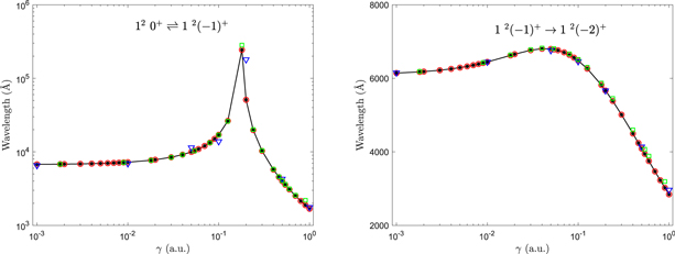
Figure 2. Current wavelengths for the two dipole transitions are compared to the other calculations (Guan & Li 2001; Al-Hujaj & Schmelcher 2004; Zhao 2018) as a function of magnetic field strengths γ. The filled dots, open dots, open squares, and inverted triangles represent the current calculations, and those of Zhao (2018), Guan & Li (2001), and Al-Hujaj & Schmelcher (2004), respectively. Note: the dots are connected with a solid line as a visual guide.
Download figure:
Standard image High-resolution imageOur oscillator strengths of the spectral lines for the two transitions as indicated in Figure 2 are compared to those from the other methods in Figure 3 with a scope of magnetic fields γ of white dwarf stars. Excellent agreement is clearly visible between the current oscillator strengths and those from our previous theoretical approach (Zhao 2018) for the two transitions. Also, the current oscillator strengths agree well with those from the modified full core plus correlation method of Guan & Li (2001), except for a small range at γ = ∼0.2 au of the transition  , where a remarkable discrepancy exists. One can see a minimum of the oscillator strengths for this transition at γ = ∼0.2 au, where the transition is relatively weak. As exact calculations of any weak transitions are very difficult, such a remarkable discrepancy is not beyond our expectation.
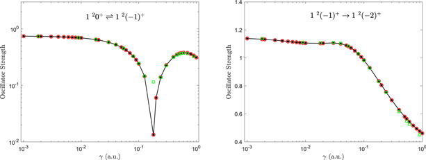
Figure 3. Same as Figure 2, but for the oscillator strengths. Comparison of the oscillator strengths is made with the results of Zhao (2018) and Guan & Li (2001), but without those of Al-Hujaj & Schmelcher (2004). Note: the dots are connected with a solid line as a visual guide.
Download figure:
Standard image High-resolution imageEven though no spectra of magnetized Li atoms are reported for the transitions to highly excited states, their experimental spectra are listed in the NIST database in the field-free cases, and the field-free theoretical spectra are published by Lindgård & Nielson (1977). In order to check the current two-dimensional B-spline approach by comparison, we calculated the field-free spectra for the transitions  with n = 2–7 and
  with n = 3–8, where Mi and Mf represent the total orbital magnetic quantum number of the corresponding atomic states, respectively. The 12 groups of these transitions contain those to both highly excited states and low-lying states. The spectral lines corresponding to all 12 of these groups of the transitions are obtained. We illustrate the oscillator strengths for the two groups of the transitions to highly excited states
  from
from  and to
  from
from  in Table 12. Similar comparison between our previous approach (Zhao 2018) and the modified full core plus correlation method of Guan & Li (2001), limited to the transitions to low-lying atomic states from
  and
and  , has been performed in Zhao (2018).
Table 12.
Field-free Oscillator Strengths f for the Two Transitions to the Highly Excited States from the Two Low-lying States, 1 and
and  , where Mi and Mf Denote the Magnetic Quantum Numbers of the Initial and Final States, Respectively
1
|
1
|
||||
|---|---|---|---|---|---|
| Mi | Mf | f | Mi | Mf | f |
| 0 | −1 | 1.009869(−3) | −1 | −2 | 1.508187(−2) |
| 0 | 0 | 1.009869(−3) | −1 | −1 | 7.540937(−3) |
| 0 | +1 | 1.009869(−3) | −1 | 0 | 2.513646(−3) |
| ⋯ | ⋯ | 0 | −1 | 7.540937(−3) | |
| ⋯ | ⋯ | 0 | 0 | 1.005458(−2) | |
| ⋯ | ⋯ | 0 | +1 | 7.540937(−3) | |
| ⋯ | ⋯ | +1 | 0 | 2.513646(−3) | |
| ⋯ | ⋯ | +1 | +1 | 7.540937(−3) | |
| ⋯ | ⋯ | +1 | +2 | 1.508187(−2) | |
| ⋯ | 1.009869(−3) | ⋯ | ⋯ | 8.378819(−3) | |
Note. The values in the last line represent the oscillator strengths averaged over all possible transitions with various Mi and Mf.
Download table as: ASCIITypeset image
The oscillator strengths for the 12 groups of the transitions are obtained by averaging the detailed oscillator strengths, relevant to the magnetic quantum number, as given in Table 12, over all possible transitions. Table 13 lists our wavelengths and oscillator strengths for the field-free cases, and comparison is made to the experimental values from the NIST database and the theoretical results of Lindgård & Nielson (1977). Good agreement is distinctly seen with these published wavelengths and oscillator strengths. Comparison performed in Figures 2 and 3 and Table 13 illustrates the reliability of the current two-dimensional B-spline approach in the calculations of spectra of lithium in the scope of magnetic fields of white dwarf stars.
Table 13. Comparison of Field-free Wavelengths λ and Oscillator Strengths f for the 12 Transitions among Our, NIST, and LN Results
| Transitions | Present | NIST | LN | |||
|---|---|---|---|---|---|---|
| λ(Å) | f | λ(Å) | f | λ(Å) | f | |

|
6709.8 | 7.482(−1) | 6707.9 | 7.469(−1) | 6710 | 7.412(−1) |

|
3235.1 | 4.658(−3) | 3232.7 | 4.712(−3) | 3234 | 4.225(−3) |

|
2742.6 | 4.235(−3) | 2741.2 | 4.218(−3) | 2742 | 3.949(−3) |

|
2563.4 | 2.538(−3) | 2562.3 | 2.620(−3) | 2563 | 2.377(−3) |

|
2476.0 | 1.558(−3) | 2475.1 | 1.581(−3) | 2476 | 1.463(−3) |

|
2426.3 | 1.010(−3) | 2425.4 | 1.012(−3) | 2426 | 9.496(−4) |

|
6102.6 | 6.367(−1) | 6103.5 | 6.386(−1) | 6105 | 6.354(−1) |

|
4603.5 | 1.229(−1) | 4602.8 | 1.230(−1) | 4604 | 1.227(−1) |

|
4133.5 | 4.637(−2) | 4132.6 | 4.650(−2) | 4134 | 4.625(−2) |

|
3916.3 | 2.300(−2) | 3915.3 | 2.283(−2) | 3916 | 2.296(−2) |

|
3796.0 | 1.324(−2) | 3794.7 | 1.314(−2) | 3796 | 1.321(−2) |

|
3721.8 | 8.379(−3) | 3718.7 | 8.353(−3) | 3722 | 8.371(−3) |
Note. Here, present denotes our results, while NIST and LN represent the experimental data from the NIST database (http://physics.nist.gov) and the theoretical data computed by Lindgård & Nielson (1977), respectively.
Download table as: ASCIITypeset image
It can be expected that the influence of magnetic fields on highly excited states should be pronounced. In order to quantitatively see such an influence, we choose an atomic state,  , and plot probability density distributions of its outer electron as a function of magnetic field strengths in Figure 4. It is easily found from this figure that the electron clouds are squeezed toward ρ = 0 in the direction transverse to the z-axis by magnetic fields, i.e., the wave functions shrink toward the z-axis, and as the field strengths increase, the field influence becomes bigger and bigger. At γ = 1 au, the probability densities are compressed by more than one order of magnitude, compared to those at the field-free case. Furthermore, we also investigated the influence of magnetic fields on low-lying states, and discovered that such an influence is remarkably smaller than that on highly excited states. Considering the competition between the Coulomb and diamagnetic potentials for the different atomic states, such a result is physically reasonable.
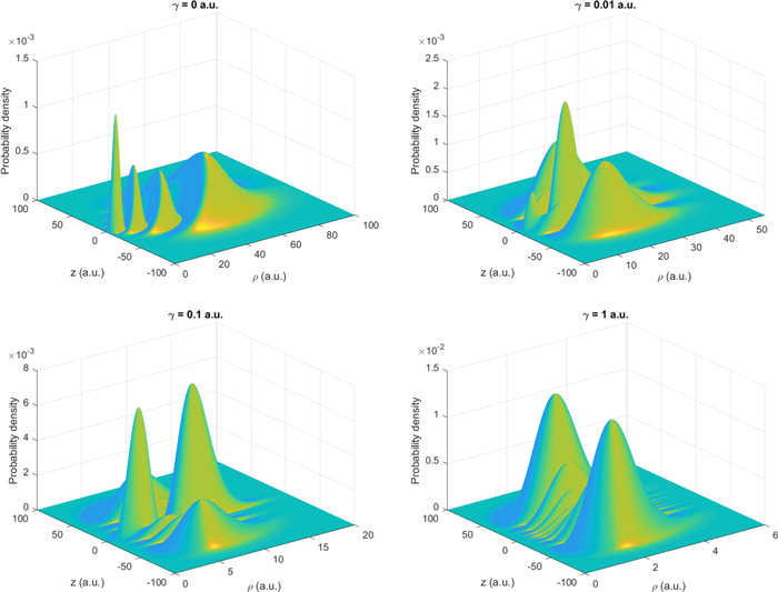
Figure 4. Probability density distributions of the outer electron for the  state of lithium atoms,
  , integrated over the angular variable ϕ of cylindrical coordinates, for the selected magnetic field strengths with γ = 0, 0.01, 0.1, and 1 au.
Download figure:
Standard image High-resolution image4. Application in Modeling Spectra of Magnetic White Dwarfs
Recently, Ferrario et al. (2015) have reviewed observational and theoretical studies on magnetic white dwarfs in the literature. It has been discovered that the number of weakly and strongly magnetized white dwarfs has increased to more than 600 up to 2015 (also see Kepler et al. 2013, 2015) from less than 70 in the early stage (Wickramasinghe & Ferrario 2000). Some of the magnetic white dwarfs with hydrogen atoms have been identified due to continuous endeavors in understanding atomic structures of magnetized hydrogen with the field strengths of magnetic white dwarfs and neutron stars (Forster et al. 1984; Schimeczek & Wunner 2014b). The magnetic fields of these white dwarfs and their geometries over the white dwarf surfaces are determined by contrasting the observed spectra with the computed ones. However, many magnetic white dwarfs with nonhydrogen atoms have not yet been identified due to the lack of theoretical spectral data of nonhydrogen atoms.
The modified full core plus correlation method established by Guan & Li (2001) and the full configuration interaction method by Al-Hujaj & Schmelcher (2004) are an attempt to understand behaviors of magnetized multielectronic atoms. Their methods treat the electron correlation problem in the presence of a strong field based on nonperturbative theory, and have a potential applied to modeling spectral lines of the magnetic white dwarfs with lithium-dominated atmospheres. Very recently, Zhao (2018) developed a theoretical approach, in which this so-called electron correlation problem in a strong field is avoided, to calculate magnetized lithium atoms. Our analysis shows that this approach is able to produce atomic spectral data of lithium in a magnetic field of white dwarfs, and our data are comparable to those reported by Guan & Li (2001) and Al-Hujaj & Schmelcher (2004). However, it should be emphasized that all these methods reported in the literature are inappropriate for highly excited states of magnetized lithium due to the limitations of these methods. The current two-dimensional B-spline approach is developed to meet the application requirements to model spectral lines of highly excited states of lithium in magnetic white dwarfs.
We would point out that although H, He (Ferrario et al. 2015), and a few relatively heavy elements, such as Na i, Mg i, Ca i, and Ca ii (Reid et al. 2000), have been identified in the atmospheres of magnetic white dwarfs, so far no lithium atoms have been discovered therein. The present work lays a foundation for the identification of lithium atoms. In particular, the current two-dimensional B-spline approach is able to be extended to calculate atomic structures of the other multielectronic atoms in a magnetic field, and thus it has a potential applied to the investigation of Zeeman spectroscopy of white dwarfs and neutron stars.
5. Summary and Conclusions
We developed a two-dimensional B-spline approach in the cylindrical coordinate system to calculate atomic structures and spectral lines of highly excited states of magnetized lithium. Energy levels are presented for highly excited atomic states  ,
,  ,
,  ,
,  , and
, and  with ν = 5–10 with a scope of magnetic fields of white dwarf stars. Spectral lines for the transitions to these highly excited states from the three low-lying states
  ,
,  , and
, and  are also calculated, and the corresponding wavelengths and oscillator strengths are presented in the magnetic white dwarf field strengths.
The field-free spectral data of these highly excited states are compared to the experimental results from the NIST database and the available theoretical ones of Lindgård & Nielson (1977). Good agreement with the NIST database is clearly visible for their energy levels, while our wavelengths and oscillator strengths agree well with those from both the NIST database and the theoretical ones of Lindgård & Nielson (1977). Since there are not spectral data of these highly excited states of magnetized lithium atoms in the literature, we performed calculations of discrete spectral lines between the low-lying atomic states to check the current two-dimensional B-spline approach by means of comparison. The present wavelengths and oscillator strengths for the low-lying states calculated with the two-dimensional B-spline approach are in line with the spectral data of Guan & Li (2001), Al-Hujaj & Schmelcher (2004), and Zhao (2018). These comparison results illustrate that the current two-dimensional B-spline approach is reliable in the calculations of lithium atoms in magnetic fields of white dwarf stars.
In view of that our previous approach (Zhao 2018) is inapplicable for highly excited states,  with
with  , of magnetized lithium due to too large Hamiltonian matrix sizes involved for such states, and the other theoretical methods for describing magnetized lithium in the literature are also limited to the treatment of the ground state and low-lying excited states, it is inevitable to establish an approach, which can be used to calculate high excited states. The current approach is developed to meet such an application requirement, and fortunately it is also valid for low-lying atomic states. In particular, it is useful to systematically produce atomic data to model discrete atomic spectra of highly excited states as well as low-lying states of lithium in the atmospheres of magnetic white dwarfs.
This work is supported by the National Natural Science Foundation of China under grant No. 11974087, the Science and Technology Platform and Talent Team Program of Guizhou province (No. 2017-5610), and the Major Research Project of innovative Group of Guizhou province (No. 2018-013).