Abstract
Observations of the Sun as a star have been key to guiding models of stellar atmospheres and additionally provide useful insights on the effects of granulation and stellar activity on radial velocity measurements. Most high-resolution solar atlases contain telluric lines that span the optical and limit the spectral regions useful for analysis. We present here a telluric-corrected solar atlas covering 0.5–1.0 μm derived from solar spectra taken with a Fourier transform spectrograph at the Institut für Astrophysik, Göttingen. This atlas is the highest-resolution spectrum with a wavelength calibration precise to ±10 m s−1 across this 500 nm spectral window. We find that the atlas matches to within 3% of the telluric-corrected Kitt Peak atlas in regions containing telluric absorption weaker than 50% in transmission. The telluric component of the spectral data is fit with a semiempirical model composed of Lorentz profiles initialized to the High-resolution Transmission Molecular Absorption Database (HITRAN) parameters for each absorption feature. Comparisons between the best-fit telluric parameters describing the Lorentz profile for each absorption feature and the original HITRAN values in general show excellent agreement considering the effects atmospheric pressure and temperature have on our final parameters. However, we identify a small subset of absorption features with larger offsets relative to the cataloged line parameters. We make our final solar atlas available online. We additionally make available the telluric spectra extracted from the data that, given the high resolution of the spectrum, would be useful for studying the time evolution of telluric line shapes and their impact on Doppler measurements.
1. Introduction
The Sun is the most well-studied star and serves as a benchmark for our understanding of stellar physics. High-resolution spectra of the Sun have been essential references for a variety of stellar and planetary studies that strive to understand atomic physics processes in the solar atmosphere (Fontenla et al. 2011; Nordlander & Lind 2017), determine the chemical abundances of other stars (Asplund et al. 2009; Bruntt et al. 2012), and measure the radial velocities of solar system objects reflecting solar light (Bonifacio et al. 2014). More recently, the use of solar spectra has been helpful to understand the effects of magnetic activity and gravitational blueshift on radial velocity (RV) measurements (Dumusque et al. 2015; Dumusque 2016; Reiners et al. 2016; Milbourne et al. 2019). These studies strive to develop ways to reduce the effects of activity on stellar spectra that can limit the achieved RV measurement precision.
An additional application of solar spectral observations is the study of telluric lines themselves since the Sun serves as a bright backlight to the atmosphere that provides enough light for high signal-to-noise ratio (S/N), high-resolution telluric measurements. This enables the study of weak telluric lines, or microtellurics, that are of additional pertinence to exoplanet RV studies owing to their ability to impact precision RV measurements (Artigau et al. 2014; Cunha et al. 2014; Halverson et al. 2016; Bechter et al. 2018; Plavchan et al. 2018). Solar spectra have also proven useful to measure abundances of atmospheric gases (Toon et al. 1999, 2018; Harrison et al. 2012) and to validate line parameter databases (Toon et al. 2016).
High-resolution, disk-integrated spectra of the Sun are difficult to obtain from space but are crucial for studies that need to view the Sun as a star. Ground-based solar atlases generated with spectrographs having resolution too low to resolve the solar lines are useful but suffer from the effects of an instrument-specific line-spread profile (LSP). The convolution of the full observed spectrum with the LSP makes telluric removal challenging since a correction by dividing a telluric model is no longer mathematically exact. Furthermore, the convolution with the LSP complicates comparisons between data and models at different resolutions.
Several ground-based instruments have been successful at observing disk-integrated spectra of the Sun at a resolution that fully resolves the solar lines. These include Kurucz et al. (1984) and Reiners et al. (2016), which both utilized Fourier transform spectrographs (FTSs). In a comparison of the wavelength solutions of these two atlases, Reiners et al. (2016) showed that errors in the wavelength calibration of the Kitt Peak solar atlas were >50 m s−1 in regions blue of 473 nm and 20 m s−1 red of 850 nm, whereas the Institut für Astrophysik, Göttingen (IAG) solar flux atlas shows good agreement to within 10 m s−1 with a HARPS laser frequency comb calibrated atlas (Molaro et al. 2013), which was taken at slightly lower resolution covering a 100 nm range around 530 nm. Comparisons of the IAG atlas with a second Kitt Peak atlas derived slightly differently from the first (see Wallace et al. 2011) shows even larger offsets.
These high-resolution, disk-integrated solar atlases are commonly used as a comparison to solar models that are important for studying non-LTE effects that change the line shapes of various molecular features, such as that of calcium (Osorio et al. 2019). Additionally, observing the Sun as a star and measuring the line bisectors provides important information for exoplanet RV studies that must understand the limiting effects of granulation and starspots on their RV measurements. For these applications, the Sun serves as a useful test case since high-resolution and high-S/N measurements can be achieved, which are necessary to compare measurements to models and study the effects of degrading the spectral resolution, as will commonly be the case for measurements of other stars (Gray & Oostra 2018; Cegla et al. 2019). Additionally, being able to image the stellar surface provides extra information in studying the effect of starspots. For all these applications, telluric lines can skew the measurements (Löhner-Böttcher et al. 2018) and limit the spectral regions that are useful for these studies (Nordlander & Lind 2017; Quintero Noda et al. 2018).
Few efforts have been made to correct solar spectra for telluric lines, possibly because this is more difficult for the Sun owing to the lack of telluric reference stars and the low Doppler shifts of the solar lines, meaning that telluric lines do not shift significantly with respect to the solar features. In work by Kurucz (2005), the Kitt Peak Solar Atlas (KPSA) was telluric corrected using a full radiative transfer atmospheric model. Residuals were replaced by hand with lines connecting the boundaries of contaminated regions. In 2011 another disk-integrated solar atlas was observed at Kitt Peak by Wallace et al. (2011), who corrected the spectrum for atmospheric absorption by using telluric data derived from disk-centered solar spectra. The improved wavelength calibration of the IAG atlas, in addition to the lack of uncertainties on the Kitt Peak atlases, motivates the derivation of a new telluric-corrected solar atlas derived from IAG solar spectral data. Here we generate this telluric-corrected IAG solar flux atlas that has estimated uncertainties that capture the success of the telluric removal process and therefore makes it useful for studies that wish to mask or properly weight telluric-contaminated spectral regions. To achieve this, we develop a unique semiempirical telluric fitting method that works well despite the small Doppler shifts of the solar lines that make it challenging to dissociate them from overlapping telluric features.
In Section 2 we describe the data set used to generate this atlas and the preprocessing steps performed to determine the wavelength calibration and solar RV for each spectrum. In Section 3 we describe the model framework, and in Section 4 we describe the fitting sequence and how we use the best-fit models to generate the output data products that include the final atlas and an archive of telluric spectra. We provide an analysis in Section 5 in which we compare our solar atlas to the KPSA and discuss our telluric model and findings related to the telluric line shape parameters. Finally, we conclude in Section 6.
2. Data
The data used here for generating a telluric-free, disk-integrated solar spectrum were taken with the Vacuum Vertical Telescope3 at the Institut für Astrophysik in Göttingen, Germany. A siderostat mounted on the telescope directs light into an optical fiber that passes through an iodine cell before feeding the FTS (Lemke & Reiners 2016). The iodine cell serves to provide a wavelength calibration that is more accurate than the internal calibration of the FTS. We utilize a subset of spectra from a 20-day data set taken over the span of a year, with each day having disk-integrated solar spectra recorded over a multiple-hour span. Additionally, 450 spectra were taken using a halogen light source with the iodine cell in order to generate an iodine template spectrum. Although the original spectra cover a slightly wider wavelength range, we only process the region from 500 to 1000 nm. The resolution of the spectra is λ/Δλ ≈ 106, and the S/N in the continuum spans from 100 to 300 over the full wavelength range. For more information on the data and instrument setup, we refer the reader to Lemke & Reiners (2016) and Reiners et al. (2016).
For generating the atlas, we choose a subset of spectra with a wide range in both solar RV and air mass in order to achieve the best separation of each spectral component by leveraging the fact that the telluric component varies with air mass while the solar component varies with RV. We opt to combine different days of data not only to maximize the range in these variables but also to leverage the different atmospheric conditions that will produce different telluric residuals and therefore reduce the possibility of confusing a telluric residual with a solar feature. We create 11 groupings of data on which we perform our fits, with each group containing 12–15 spectra. Before running these fits, we perform several preprocessing steps on the full sample of data that we describe below.
Flux Normalization.—We first prepare the data for fitting by dividing out the continuum to produce spectra with normalized flux levels. We do this individually for each spectrum using an automated process that steps through 150 cm−1 subregions for each spectrum and records the maximum flux value and corresponding wavenumber value. A cubic spline is fit to these ∼70 points that describe the continuum. The raw flux data are divided by this spline description of the continuum in order to produce the final normalized flux data. Any errors in this process are accounted for in our ultimate fitting sequence by including a floating linear continuum correction.
Prefits: Solar and Iodine Velocities.—Using these flux-flattened spectra, we perform a fitting routine that determines (1) the solar velocity offset, v, relative to a template solar spectrum and (2) the wavelength calibration from the iodine lines using νc = ν(1 + κ), where νc is the corrected frequency array, ν is the original frequency array, and κ = −viod/c, where viod is the iodine velocity and c is the speed of light. We determine these values a priori instead of optimizing them simultaneously with our telluric fitting sequence in order to enforce these values to be the same between the narrow (10 cm−1) wavelength regions over which we perform each telluric fit. This ensures that we are fully leveraging our knowledge of the locations of the stellar lines, which is particularly important in regions that do not contain strong stellar features. The fitting routine we use to determine v and κ for each spectrum follows the method described in Section 3 of Lemke & Reiners (2016), except instead of using an iodine-free IAG solar template, we use the telluric-corrected KPSA since we later use this for our starting guess of the solar spectrum in our full (solar+telluric) fits to the data. Although it is not necessary to begin with a solar model, this speeds up the iterative fitting process.
In Figure 1 we show several parameters determined for a sequence of observations taken on 2016 February 27. In the top panel of Figure 1 we plot the measured velocities of the solar lines. The scatter in the measured solar velocity values is structured owing to tracking errors, sunspots, and physical sources of line shifting that can occur (see Reiners et al. 2016 for more description). We ultimately shift our solar spectra by the Doppler velocity between the Sun and Göttingen calculated using the JPL ephemeris generator4 (shown in Figure 1 as the black dashed line); therefore, these effects do not affect the alignment of our final solar atlas, and the random nature of the differences in the line shapes caused by tracking errors and sunspot position, for example, will be reduced owing to averaging.
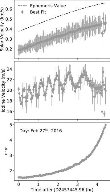
Figure 1. Observer–Sun velocity (top), iodine velocity (middle), and water vapor optical depth times air mass (bottom) vs. time for observations taken on 2016 February 27. The dashed line in the top panel shows the actual solar velocity values that were calculated using the JPL web server and are offset from our measured velocities (gray points) owing to the different zero-point velocities of the data and the template spectrum used to determine these values. The sequence of iodine velocities, measured by the iodine lines’ positions relative to a template iodine spectrum, shows the drift in the FTS over this multihour observing run.
Download figure:
Standard image High-resolution imageAn example sequence of κ values is shown in the middle panel of Figure 1, where the error bars depict the standard deviation of the values measured for each of the 10 350 cm−1 wide spectral regions that were fit independently and then averaged to determine the final iodine velocity. The average uncertainty in the measurements for this day is 0.9 m s−1, which is typical of other days of observations. The oscillatory behavior in κ is also seen in the other observing runs and shows the intrinsic drift of the instrument.
Prefits: H2O Optical Depth.—In the bottom panel of Figure 1 we show the product of air mass, α, and water vapor optical depth, τ, which accounts for the different column densities of water vapor between the various observations. The value of τ is first estimated from measuring the line depth of an isolated water vapor line located at 15,411.73 cm−1 and then further optimized in step 1 of our full fitting sequence, which is described in Section 4. We only perform these optical depth fits for water vapor since oxygen is well mixed in the atmosphere; therefore, using the air-mass values of the observation to scale the oxygen telluric spectrum to the different observations is sufficient. This is described more in Section 3.1.3.
Noise Determination.—Quantization noise, photonic noise, and instrumental noise all contribute to the final noise in our FTS spectra. Of these, photonic noise dominates at high resolution, where the informative component of the interferogram is small and can easily be swamped by the photonic noise owing to a constant term related to the half-power of the source (Barducci et al. 2010). While in theory the noise of our measurements can be calculated, it is simple and accurate to deduce the final measurement noise by measuring the flux rms of a portion of featureless spectrum. We do this for each observation by taking the noise for each spectrum to be the rms of the flux-normalized spectra over a 1.5 nm wavelength range starting at 1048.8 nm, which gives the noise in the continuum to be about 1%. This region was chosen for its lack of solar and telluric features, but it must be noted that the actual noise levels vary slightly across the full wavelength span of the data owing to the presence of telluric lines and variations in the sensitivity of the FTS. The rms in the continuum drops to 0.3% around 680 nm and increases again at bluer wavelengths. Not accounting for the varying sensitivity of the FTS does not significantly affect the performance of our fits; however, it is important to modify our noise array over regions where the transmission drops owing to saturated absorption lines. For this, we increase the noise determined for the continuum, σcont, by a range of factors such that it is equal to 1.25σcont–10σcont for where the transmission drops to 4.0%–0.3%, respectively. For example, in regions where the transmission is less than 1%, we multiply the noise array by a factor of 2.5. The factors were chosen to match the observed noise in the data. We propagate the final noise array, σ, determined using the linear normalized flux,  , to the noise of the logarithmic flux by
  and use these values in evaluating the optimization function for our fits.
3. Modeling Methods
Here we describe our model and justify our choices for how we represent each spectral component.
3.1. Model Representation
To fit the IAG solar spectra, we construct a model that is composed of solar, telluric, and iodine spectral components in addition to a linear continuum model. We represent each component in units of absorbance for the fitting process. For computing reasons, we split each spectrum into 10 cm−1 chunks that are fit separately. For each of the 11 groups of data, we simultaneously fit 10–15 spectra that range widely in the air mass of the observation and the Sun–observer velocity in order to best separate the telluric and solar components of the data. These groupings and their respective parameters are listed and described in Table 1. We therefore generate a model that is an Nspec × Npoints array, where Nspec is the number of spectra being fitted and Npoints is the number of data points in the fit region. Each model along the Nspec axis is generated using the same underlying solar and telluric spectral models but is shifted and scaled according to the solar RV and the species’ column densities (including the air-mass factor and τ for water vapor), respectively. Our final calculated model,  , for each spectrum, indexed by i, can be represented as a sum of each component in units of absorbance:

where we have used the subscripts T for telluric, S for solar, I for iodine, and C for the continuum, and absorbance,  , is just the logarithmic flux,
  . We demonstrate our model decomposed into all of these components in Figure 2, in which we have plotted the data,
  , as red points and our model, here
  , as the dashed black line, where both have been converted to linear flux units before plotting.
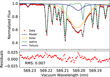
Figure 2. Example fit showing the various spectral components of our model. The continuum is not shown but is near unity for this region. The data are shown as red points with the model as the dashed black line, which is equal to the product of the telluric (navy), solar (yellow), and iodine (green) spectra. The residuals (data minus model) are shown in the bottom panel.
Download figure:
Standard image High-resolution imageTable 1. Summary of Spectral Parameters for Each of the 11 Fitting Groups
| Group |

|
vmin–vmax | τmin—τmax | αmin–αmax |
|---|---|---|---|---|
| No. | (m s−1) | (km s−1) | ||
| 0 | 4.1 | −0.1–0.3 | 1.0–5.3 | 1.1–3.5 |
| 1 | 6.0 | −0.5–0.4 | 0.3–1.3 | 1.1–3.0 |
| 2 | 1.2 | −0.1–0.4 | 0.4–2.5 | 1.1–3.0 |
| 3 | 9.4 | −0.7–0.4 | 0.2–1.0 | 1.1–3.1 |
| 4 | 3.7 | −0.1–0.4 | 0.5–2.7 | 1.1–3.1 |
| 5 | 8.8 | −0.7–0.4 | 0.3–1.7 | 1.1–3.2 |
| 6 | 2.7 | −0.6–0.5 | 0.6–3.4 | 1.1–3.2 |
| 7 | 9.4 | −0.5–0.4 | 0.4–2.2 | 1.3–3.4 |
| 8 | 8.5 | −0.7–0.5 | 0.3–1.9 | 1.1–3.4 |
| 9 | 6.9 | −0.6–0.3 | 0.4–1.6 | 1.2–3.4 |
| 10 | 5.8 | −0.7–0.4 | 0.3–1.5 | 1.1–3.5 |
Note. For the observations included in each group we report the average value of the iodine velocity ( ) in addition to the minimum and maximum values for the range of solar velocities, water vapor optical depths, and air-mass values.
Download table as: ASCIITypeset image
3.1.1. Iodine Component
For the iodine spectrum, we use the flux-normalized template spectrum made from averaging together 450 iodine spectra taken with the FTS with a halogen lamp light source. The iodine template spectrum,  , is shifted by the predetermined wavelength calibration, κ, that was found for each spectrum (see Section 2) before being added to the final model using a cubic interpolation. There are therefore no optimization parameters related to the iodine model. We point out that we chose not to simultaneously solve for κ in our full fits since the estimates from the wider wavelength regions in the prefits are more reliable than fitting for the iodine line shifts in each 10 cm−1 chunk simultaneously with the other parameters. This is particularly true in regions where few or no iodine lines exist, which is around half of our spectral range. The final iodine spectrum for each observation is described by the following equation:

3.1.2. Continuum Model
The continuum component of the model is important in order to capture errors in the flux normalization process, which is a challenge in regions where the continuum is not well defined owing to saturated telluric lines or a deep stellar feature. Because we are working in 10 cm−1 chunks that are small compared to the curvature owing to continuum modulation artifacts from the instrument, a linear trend sufficiently captures these errors. The continuum is specified in absorbance by two endpoint parameters, ξl and ξr, and an extra vertical shift specified for each date, ξdate, so that

where νl and νr are the corresponding leftmost and rightmost wavenumber values, respectively. ξdate is added to account for differences in the flux normalization process due to changing telluric absorption and differences in the illumination of the instrument, which both result in slight continuum offsets between the spectra. These continuum differences are similar for observations taken on the same day, so we only add an extra vertical shift per unique observation date that is applied to the spectra taken on the respective day.
3.1.3. Telluric Model
In the spectral range of our data, O2 and H2O are the only species whose atmospheric abundances and absorption strengths result in signals that exceed the noise of our data. We therefore only include these two species and choose to model each individual line with a Lorentz profile. We use the High-resolution Transmission Molecular Absorption Database (HITRAN), version 2016 (Gordon et al. 2017), for a starting guess to the strength, S0, width,5 γ, and center position, νc, and then optimize these parameters individually. We discuss our reasoning for pursuing this semiempirical telluric model in Appendix A.
We optimize the Lorentz parameters for all individual line transitions with S0 greater than 10−26 and 10−28 for water vapor and molecular oxygen, respectively, in HITRAN units of line intensity6
(cm−1 molecule−1 cm−2). These parameters are queried directly from HITRAN using the HITRAN Application Programming Interface (Kochanov et al. 2016). We also include in our model H2O absorption features down to S0 = 10−28 cm−1 molecule−1 cm−2, which are not individually optimized but do adopt a common modification on their line parameter values from an initial fitting step where all lines are shifted and scaled in unison. This line strength range corresponds to a linear flux approximately between 0.01% and 1% deep with respect to the continuum for the highest air-mass observations in this data set. Different threshold values for each molecule are required owing to their differing abundances in our atmosphere, Ψmol, which are multiplied by each individually optimized S value to determine the final line absorption strength. We summarize the full telluric model below, where we have indexed the H2O lines by l and the O2 lines by m, where there are  water vapor lines and
  molecular oxygen lines in total:
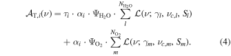
As before, each spectrum in the fit is indexed by i, and there are Nspec total. For each species, we have one principle spectrum per day that is scaled to each solar observation by the air mass, αi, and for water vapor we additionally scale by the prefitted water vapor optical depth, τi, previously determined for each observation. Although the telluric spectrum should be shifted by ki, we do not include this since any bulk shift due to differences in instrument drift across spectra (<10 m s−1 maximum; see Column (2) of Table 1) will be small compared to a modification on νc (15–500 m s−1) and will also ultimately be absorbed into the corrections on νc. As will be discussed more in Section 4, the line parameters are first all modified simultaneously with all γ values being multiplied by fγ,mol for each molecule, the line strengths being multiplied by Ψmol, and the line centers being shifted by  , where P is optimized and is physically motivated as a one-dimensional pressure term and δair is the pressure-induced shift (units of cm−1 atm−1) and is provided in the HITRAN database for each line transition.
3.1.4. Solar Model
For our solar model, we use a cubic spline that we initialize to a flux-normalized version of the telluric-corrected KPSA. The flux normalization for the KPSA is performed by simply dividing each 10 cm−1 chunk by the maximum value in that spectral range. This performs well outside regions containing very wide stellar features; however, the continuum component of our model accounts for these offsets and is later used to correct for them. We describe this in step 3 of Section 4.
Our spline is implemented using BSpline in the Python scipy.interpolate package and can be described as

Here we define the spline for a chunk of spectrum over which we define knot points, tj. The final spline function can be written as the sum of coefficients, cj, multiplied by each basis spline,  , which are defined in Appendix B.
For our application we use a cubic spline (q = 3) and position knots at intervals of 0.1 cm−1 in regions with low stellar absorption (<10% absorption) as determined by the Kitt Peak telluric-corrected solar atlas and use a knot spacing of 0.05 cm−1 for stellar spectral regions with greater than 10% absorption. We found that this knot sampling was able to capture the curvature of the spectral features and a coarser spacing of knot points would introduce oscillatory numerical features above the noise in regions with high curvature. Because each knot point has multiplicity 1 (no overlapping points), our resultant stellar spectrum will be smooth, as desired. In our fits, we optimize the coefficients, cj, of the spline that are initialized by performing a least-squares minimization between the spline and the telluric-corrected KPSA.
The final stellar model array,  , contains Nspec stellar models each shifted by the solar and iodine velocity already measured for each spectrum included in the fit. We generate
  by simply evaluating our solar spline at the array of wavenumbers modified by κi and vi:

4. Fitting and Processing Steps
Here we discuss the fitting sequence in detail and describe how we generate the final solar atlas in addition to the telluric spectra extracted from the data set.
4.1. General Fitting Routine
Step 1: Telluric Optimization.—The optimization sequence begins by stepping through the spectra in 10 cm−1 chunks (each contains 664 data points) and for each chunk fitting Nspec spectra with the solar spectral model set to the KPSA for that region while we iteratively optimize7
the continuum and telluric parameters. For this we minimize a χ2 term with a penalty term, p1, added in order to encourage the model to go to zero in saturated regions that otherwise do not contribute significantly to the χ2 value owing to the large flux uncertainties. If  is the objective function for step 1, it can be summarized as
  , with χ2 and p1 defined as follows:


Here we have denoted the number of saturated points in the fit region as Nsat and the median uncertainty over each spectrum as σmed. We include σmed to provide a scaling according to the noise in each spectrum without diminishing the term, as would happen if we used the σ values, which are large over those saturation regions. In Table 2 we summarize the parameters used to define each model component.
Table 2. Summary of the Optimization Parameters for Our Model Described in the Text
| Model | Optimized | Prefit |
|---|---|---|
| Component | Parameters | Parameters |

|
cj | vi, κi |

|
See Table 3 | τi |

|
ξl, ξr, ξdate | ⋯ |

|
⋯ | κi |
Download table as: ASCIITypeset image
For the iteration series, we begin by optimizing the continuum parameters, fγ,mol and Ψmol for each species, and P, which scales the line-center shifts. Lines with strength greater than 10−28 for both species are included in the model and are modified based on the best-fit values of fγ,mol, Ψmol, and P, which effectively modifies all features in unison. This unified shift and scaling serves as a first approach to the best-fit solution and is additionally useful for the weakest features that have line depths near the noise, making them challenging to fit individually. In the next stage, we optimize the continuum and telluric models, where all three parameters for each line of the telluric model are allowed to vary individually. As recorded in Table 3, we optimize the line parameters for individual lines with strengths greater than 10−26 and 10−28 for water vapor and oxygen, respectively. We split the water vapor lines into two groups based on line strength, which may be fit separately to improve computation times: these are a “weak” group and a “strong” line group. The lines in the “strong” group8
include absorption features with S 10 times the lower thresholds just defined for individually fitted H2O lines, with the “weak” group containing the remaining features ( ). We iterate between fitting these two telluric groups and the continuum parameters until convergence (i.e., no significant changes in the
  value). At the end we allow both groups of telluric lines and the continuum to vary simultaneously, having kept fγ,mol, Ψmol, and P fixed in this iteration process. We note that we bound the amount that the line centers can shift to 0.01 cm−1 in each optimization stage to avoid the fits swapping features in the data.
Table 3. List of Telluric Model Parameters Relevant to Select Absorption Features Depending on Their Transition Line Strengths
| Species | Line Strengths | Optimized Parameters |
|---|---|---|
| H2O | S < 10−28 | (Omitted) |
| S > 10−28 |
 , ,  , P , P |
|
| S > 10−26 | γl, Sl, 
|
|
| S > 10−25 | (“Strong” lines) | |
| O2 | S < 10−28 | (Omitted) |
| S > 10−28 |
 , ,  , P, γm, Sm, , P, γm, Sm, 
|
|
| S > 10−27 | (“Strong” lines) |
Note. We additionally denote the line strength cutoff for weak telluric features that are omitted from the model and additionally define the minimum line strength defining the boundary of the “strong” group of features that are fit together with the solar spline model in step 2 of the fitting sequence (see text for more description).
Download table as: ASCIITypeset image
We find that our fits perform well but that the optical depths of the water vapor lines are poorly estimated by our initial effort that determined τ by fitting one isolated water vapor line. We improve this by iterating between fitting for τi over all spectra and performing the fitting sequence described here until convergence. We only do this for one 10 cm−1 wide range of spectra starting at 11,010.0 cm−1 (907.44–908.26 nm), for which the region is dominated by deep water vapor lines. We find that the wings of the lines are very sensitive to the value of τ and fitting multiple lines at once significantly improves our estimates of the optical depth for each spectrum.
Step 2: Solar and Telluric Fitting.—Using the best-fit estimates for the continuum and telluric line parameters, we now optimize both the spline coefficients and the group of strong telluric transitions. We choose not to fit the weak group simultaneously with the spline optimization since these lines are fit reliably well in step 1. To perform this fit, we use the optimization function from step 1 and add another penalty term that serves to penalize the fit for adding features to the solar spectrum over saturated regions. This is to alleviate the potential problem of the spline filling in saturated regions, where no photon information exists. The two penalty terms together therefore ensure that the core of a saturated line is fit properly (i.e., the model goes to zero) while avoiding the scenario where a narrow, deep feature in the spline fills in the core, since this is unlikely and in any case cannot be constrained. We choose not to completely prevent solar features in these regions since a solar line will often overlap the edges of saturated regions and we wish to not compromise the shape of these features by abruptly forcing the spline, which must be smooth, to zero. We therefore define the penalty, p2, as

where the coefficient β is a scaling factor that adjusts the penalty term to an effective range that does not force the solar spectrum to zero but still prevents large, unnecessary additions to the spectrum. The objective function for step 2 can be summarized as  . Because we have a good first guess to the solar spectrum and our χ2 value, tuning β uniquely to each portion of spectrum can be done based on this prior information. Since our χ2 value is in theory at best unity when the residuals only encompass noise on the magnitude of the noise of the data, we can define β to be the value such that the initial penalty term is 0.5 or around 50% of χ2 for a well-optimized fit. We therefore set
  , where
  is the initial solar spectrum that has been set to the KPSA. This method of tuning a penalty term is typical in cases where overfitting can potentially be an issue (e.g., Bedell et al. 2019). The final fitting procedure works well even in saturated regions as can be seen in Figure 3 in which we show an example fit and the corresponding residuals after performing steps 1 and 2.
Step 3: Correcting the Continuum.—As noted before, the fitting process is performed for each 10 cm−1 subregion separately. Before removing the continuum, telluric, and iodine solutions to extract the final solar spectrum, we must address the fact that the continuum solution contains the corrections to both the data and solar spectral continua. We find that in saturated telluric regions the original continuum corrections are due to errors in the flux normalization done to the data, while the solar spectrum normalization process only fails for regions where the entire spectral chunk contains a wide solar feature that spans the 10 cm−1 subregion, since otherwise the solar model is at maximum (unity) between stellar lines. Over our wavelength range, there are five occurrences of a wide solar feature, and these all are present in regions that do not overlap saturated telluric features. We utilize this in separating the continuum offsets originating from the stellar model from offsets due to the continuum correction performed to the data.
To remove the offsets in the continuum solution due to errors in the initial normalization to the solar spectrum, we take the final best-fit continuum array, and if the spectral subregion under consideration is overlapping a dense telluric band, we leave the continuum alone. If the subregion does not contain dense9 telluric features, we modify the best-fit continuum model by subtracting from it the median value of the continuum solutions determined for each spectrum in the group. Because we will later use the solar spline model to replace regions containing telluric residuals, we add these subtracted values to our stellar spline model. This transfers any continuum offsets originating from the stellar normalization process back to the stellar spectrum, while keeping information about the relative offsets between the spectra grouped by date. Typically these offsets are small over telluric-free regions.
4.2. Generating the Final Solar Spectrum
Removing Best-fit Model Components.—Using the corrected continuum array along with the telluric model and iodine template, we can subtract these from the FTS data to leave just the solar component:

Here we have denoted  as our corrected continuum array and
  as our final solar spectra for each observation defined over our full wavelength span, and we have converted from absorbance to transmission. We note that in regions where the data are saturated there will be spurious values due to dividing regions dominated by noise by the model that is approximately zero in those regions. Residuals from the telluric subtraction may also remain in the final solar spectrum and are typically visible over deeper lines (>10% absorption). Instead of excising these regions entirely, we replace them by our spline model. These regions are flagged in the final spectrum.
Velocity Zero-point Determination.—To achieve an absolute wavelength calibration, we use the iodine catalog from Salami & Ross (2005), who recorded a Doppler-limited iodine spectrum using an FTS and corrected the wavelength scale to match other wavelength-calibrated iodine atlases, including that of Gerstenkorn & Luc (1981). From their comparison to these other atlases, they estimate that their spectrum is reliable to ±0.003 cm−1 across their frequency range of 14,250–20,000 cm−1. We use their recorded spectrum to find the offset of our template iodine spectrum and find that our iodine spectrum is shifted redward of the template by about 70 m s−1, or 0.004 cm−1. We shift our final solar spectrum by 70 m s−1, such that κ = 2.3 × 10⁻⁷, and adopt the uncertainty in the template iodine spectrum of ±0.003 cm−1, which translates to ±45 m s−1 at frequencies of 10,000 cm−1 and ±90 m s−1 at 20,000 cm−1. We note that any shifts in our iodine spectrum due to a temperature difference between our setup and the temperatures used by Salami & Ross (2005) should be over 10 times smaller than our adopted uncertainties for the absolute shift of our final stellar spectrum (Perdelwitz & Huke 2018). We additionally attempted to derive a zero-point offset solution using the central positions of the telluric lines as compared to their catalog line center modified by the pressure-induced line shift. This produced a consistent result but was less precise. This is described more in Appendix C.
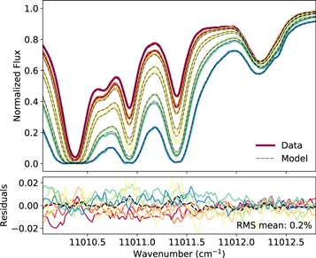
Figure 3. Example fit shown for a small wavelength region for one group of spectra. The flux-normalized spectra are shown with colors corresponding to the water vapor optical depth, and the best-fit models for each are plotted as a dashed black line (top). The residuals for each fit are shown (bottom) with the same colors. A solar feature on the right is apparent owing to its lack of change with air mass and demonstrates the small Doppler velocities that cause line shifts smaller than a fraction of a line width.
Download figure:
Standard image High-resolution imageCombining Spectra.—We combine our spectra after shifting  according to the velocity
  between Göttingen and the Sun at the time of the observation. We also perform a second shift for the calibration velocity measured from the iodine lines and the final shift for the absolute zero-point velocity. We combine the spectra by stepping through the same 10 cm−1 chunks and, before averaging, remove spectra with extreme residuals due to either a poor fit or a large air-mass value that, although they are useful for constraining the spline fit, have higher uncertainties and the least information over telluric regions. We record the final average of the remaining spectra as our telluric-free IAG solar flux atlas and record the standard deviation of these remaining spectra as the final uncertainty. We plot the final atlas in Figure 4.
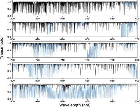
Figure 4. Transmission as a function of wavelength for the full telluric-corrected IAG solar atlas. In black is the final solar spectrum, and in blue is an extracted telluric spectrum. The telluric model shown is typical of conditions at Göttingen (precipitable water vapor of ∼10 mm).
Download figure:
Standard image High-resolution imageFor ease of use and since the uncertainty array will fail over telluric-contaminated regions replaced by the spline model, we create a flag array for the final solar spectrum to identify regions with varying levels of telluric absorption: 0 indicates a robust spectral region, 1 indicates a region with telluric absorption exceeding 10%, 2 is for telluric absorption exceeding 25%, and 3 is for saturated regions. Of these, flags greater than or equal to 1 correspond to regions that have been replaced by the spline model.
We inspect the final solar atlas and notice that the oxygen A bandhead and the area around the HeNe laser used for internal wavelength calibration of the FTS both contain spurious features. We excise these two regions (14,522.0–14,523.6 cm−1 for the O2 residuals and 15,795.1–15,799.0 cm−1 for the HeNe residuals) by replacing them with unity and assigning zeros to the uncertainty array and a flag value of 3 for the full extent of both regions. We also point out that several deep solar lines in the 500–555 nm (18,000–20,000 cm−1) range were very close to saturated such that if an iodine feature overlapped the deepest portion, the final division of the iodine spectrum would leave a large residual in the solar spectrum. Since the iodine features are stable in time, the solar spline model occasionally fit the residuals such that the model could not be reliably used to replace the erroneous spectral shape. A few near-saturated solar lines therefore contain poorly constrained line core shapes; however, the final uncertainties capture the magnitude of these deviations.
4.3. Extracting Telluric Spectra
The high resolution and high S/N of the IAG solar spectra make it a good data set for various telluric line studies. For example, this may include studying commonly used telluric modeling codes, the stability of oxygen lines, and the impact of microtelluric lines on RV measurements. We therefore create solar-corrected telluric spectra from the data set and also make these publicly available for future studies. To do this, we divide the linear flux-normalized data by the shifted iodine spectrum and by the final stellar model shifted by the solar velocity determined from the prefits. We then shift each spectrum by its iodine velocity, κ, and the zero-point velocity and then save each spectrum recorded with the air mass and our measured water vapor optical depth values for the observation. We recommend the solar spectrum be downloaded and referred to as well, depending on the use of the telluric spectra since overlapping solar lines could potentially skew the shape of an extracted telluric spectrum.
We make available the solar and telluric data products online.10 In Figure 4 we show the final solar atlas covering 500–1000 nm in black, with an example telluric spectrum extracted from the data in blue.
5. Analysis and Discussion
Here we compare our final solar atlas to the KPSA and discuss our telluric fits. We additionally compare our best-fit telluric model parameters to the starting HITRAN values and comment on several observations.
5.1. Comparison to the Kitt Peak Atlas
We compare our final spectrum to the KPSA that we used as a starting guess to our solar spline model and note that the bulk of the differences occur over dense telluric bands, as expected. This can be seen in Figure 5, in which we plot the residuals between the two solar spectra. In regions overlapping telluric features <50% in depth, we observe that the differences are <3%. Spectral features overlapping saturated or near-saturated lines occasionally differ by as high as 25% or more. Inspecting the differences between the two spectra over strong telluric lines shows (a) similarly identified features differing in line strength and/or shape and (b) solar features present in one atlas but not in the other. We show examples of these cases in Figure 6.
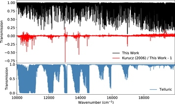
Figure 5. Comparison of Kitt Peak and IAG telluric-corrected solar atlases. The top panel contains the IAG best-fit solar spline model (black) and the residuals between Kurucz (2005) and the spline (red). In the bottom panel we show a telluric model in blue.
Download figure:
Standard image High-resolution image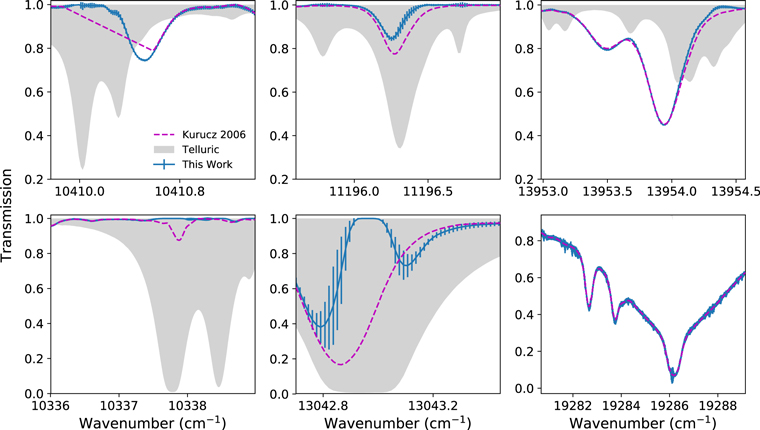
Figure 6. Comparison of Kitt Peak and IAG telluric-corrected solar atlases over select wavelength ranges. Uncertainties are generated by taking the standard deviation of all telluric-subtracted spectra used to generate the IAG solar flux atlas.
Download figure:
Standard image High-resolution imageMost of the differences in the line shapes occur due to bordering saturated telluric regions, over which we have no information and our algorithm encourages solar lines to return to the continuum, which can sometimes split a solar line in two (e.g., bottom middle of Figure 6). This was expected, and the saturated flag we provide can be used to ignore the erroneous section of the line. We do see that sometimes our solution finds a narrower line over nonsaturated lines (top middle and right of Figure 6) than in the KPSA, though we note that the reverse case happens as well.
In Figure 5, where we plot the residuals between the two spectra, we notice that more residuals fall below zero, corresponding to the KPSA typically having lower transmission than our spectrum in discrepant regions. A partial explanation is that our algorithm will return to the continuum in saturated regions where there is no information otherwise. Also, occasionally Kurucz (2005) would replace regions that had remaining large residual features with a linear interpolation that connects the adjacent regions. Our spline in contrast would smoothly return to the continuum level (e.g., top left of Figure 6).
In the blue region of our spectrum (wavenumbers higher than 17,500 cm−1) it can be seen that there is more scatter in our solution compared to the KPSA. This is due to higher instrument noise in this region, as well as iodine features that were poorly removed. Because the iodine cell was not temperature stabilized at the time these data were observed, the line strengths of the iodine lines in the template spectrum differed slightly from the iodine strengths in the data. Nevertheless, the uncertainties in the final solution account for this (e.g., bottom right of Figure 6).
5.2. Missing Water Vapor Lines
Three prominent spectral features were found that were unaccounted for in our model. For each feature, we correlated the integrated line absorption with air mass and determined that all are telluric in origin. Furthermore, we find that each has a one-to-one correlation to the integrated strength of a water vapor feature of similar depth, which confirms that all are water vapor lines. We add these lines to our local HITRAN water vapor database before performing the fitting sequence in these regions. We initialize the fitting parameters for each line to those of lines similar in strength and summarize these values in Table 4. We queried the HITRAN 2016 database around the line centers but did not find any other possible candidate species having large enough strength to explain the features. We note that the HITRAN line lists are extensively complete, especially for water vapor over optical wavelengths, and so it is possible that these lines were accidentally omitted between versions, as we see no reason that these lines would be missed in the detailed laboratory experiments that source the HITRAN line lists. These three lines were the only ones found missing, although we estimate that we would be limited in our ability to detect missing lines weaker than about 0.5% in the continuum and about 2% over other features, since this is on the order of the residuals in the continuum and over some telluric lines, respectively. Additionally, we sometimes find that some dense saturated regions are easily fit very well, while some regions leave larger, structured residuals that could be due to a missing telluric feature or an overlapping solar line, but we do not have the ability to determine the true cause.
Table 4. Telluric Lines Found Unaccounted for from Our HITRAN 2016 Input Parameters
| Line Center | Initialized Strength | Initialized Line Width |
|---|---|---|
| (cm−1) | (cm1/(molecule cm2)) | (cm−1 atm−1) |
| 10,519.8 | 4 × 10⁻²⁴ | 6.3 × 10⁻² |
| 13,941.4 | 1.76 × 10⁻²⁴ | 8.8 × 10⁻² |
| 13,943.0 | 1.76 × 10⁻²⁴ | 8.8 × 10⁻² |
Download table as: ASCIITypeset image
5.3. Comparison to HITRAN
The HITRAN line lists are a vital resource to many scientific studies from modeling Earth’s atmosphere to remote detection of a molecular species. The water vapor line lists are of particular importance owing to the role water plays in Earth’s atmosphere and its large absorption features across the optical to near-IR (NIR) spectrum. A large amount of theoretical and laboratory work has gone into improving these line parameters, particularly for water vapor (Ptashnik et al. 2016; Gordon et al. 2017). Additionally, comparisons between atmospheric absorption data and HITRAN databases have been performed, demonstrating overall excellent agreement, but identifying some regions with small differences between some HITRAN releases and observed line shapes, strengths, and locations (e.g., Bean et al. 2010; Toon et al. 2016). Several atmospheric modeling codes for astronomical applications rely on HITRAN (e.g., Bender et al. 2012; Bertaux et al. 2014; Gullikson et al. 2014; Smette et al. 2015). Discrepancies at the 1%–5% level between observations and theoretical telluric models may be found when using older versions of the HITRAN database, although such discrepancies can also stem from the specific implementation of the radiative transfer calculation. In certain spectral regions, particularly in the region between the optical and NIR, the on-sky and laboratory data and calculations underlying HITRAN database parameters may not be as robust as they are in the optical. It is therefore interesting to compare the results of our simplified telluric fits to the HITRAN database values. We do this only for water vapor owing to the complexities and smaller number of lines in the case of molecular oxygen.
While our parameters are not accurate measures of the true underlying line parameters, we still expect to see trends between our line parameters and the physical quantities that describe how these lines vary with pressure and temperature. For example, in Figure 7 we show the difference between our best-fit line centers and the HITRAN catalog starting value plotted against the δair parameter that describes the magnitude of a pressure-induced shift for a given line. Line transitions with a larger δair value will shift more at a specific pressure, which we observe. Since we fit multiple spectra simultaneously that were taken on different days and therefore under different atmospheric conditions, this induces extra scatter from averaging over different pressures and temperatures. However, since this trend largely depends on pressure, and higher in the atmosphere the pressure is consistently lower than the HITRAN reference pressure, the scatter induced by this fact does not wash out the overall trend. We note that we also see a correlation between the lower-state energy level (elower) and the ratio of our optimized line strength to the HITRAN line strength values. However, this trend is slightly weaker owing to other factors that determine how line strength changes. The same is true for the correlation between the line width ratio and nair, the coefficient of temperature dependence on line broadening.
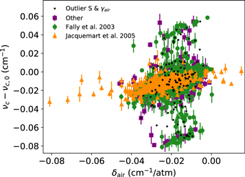
Figure 7. Best-fit line centers minus the HITRAN value for H2O as a function of δair, the pressure-induced line shift. Data points are colored by select references. The data are averaged together from separate fits, and points with errors higher than 0.01 cm−1 are removed for clarity. Black stars indicate independently selected points that have outlier line strengths and widths in comparison to the HITRAN values.
Download figure:
Standard image High-resolution imageIn making these comparisons, we observe a handful of outliers that are apparent in Figures 7 and 8. For the line centers, we see one group shifted 0.07 cm−1 downward and another shifted 0.05 cm−1 upward in frequency. Some of these correspond to lines that are also outliers when comparing γ from our Lorentz fit to γair from the HITRAN database (shown in Figure 8), as well as being discrepant in the line strength parameter, S. These lines are mostly located between 0.9 and 1.0 μm, which contains a strong water vapor band and has many saturated lines that often overlap, making them difficult to fit and also introducing degeneracies in the best-fit solution. Weak, unsaturated absorption features overlapping saturated regions would also have poorly constrained line centers. An inspection of a subset of outlier points confirms that some of the outliers result from saturation issues. A subset can also be attributed to lines that border the edge of a fitting subregion and therefore are also poorly constrained. These outliers resulting from fitting-related causes show higher variance in their mean value determined from the 11 fits, as would be expected. However, another set of discrepant points exist that exhibit small variation in their line parameters between fits and under inspection are isolated or minimally blended with a neighboring line such that the most likely explanation for the discrepancy is the HITRAN catalog value itself. These lines are found across the entire spectral range analyzed here. We color the points in Figures 7 and 8 by the most common references for the parameters δair and γair, respectively, but do not find that one source was the cause of the offsets, although the more recent works colored in orange in both plots (Jacquemart et al. 2005; Gamache & Hartmann 2004) show less scatter. A more detailed study of these parameters could elucidate the observed discrepancies. For example, fitting the telluric output spectra from this work with a full atmospheric modeling code such as MOLECFIT (Smette et al. 2015) or TERRASPEC (Bender et al. 2012) would be a good framework for validating the results from this analysis.
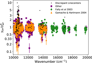
Figure 8. Best-fit Lorentz widths over the original HITRAN database air-broadened γ value plotted vs. wavenumber for H2O and colored by select references. Data points are the average from several fits, and points with statistical uncertainties greater than 2% are removed. The black stars are independently selected lines that have discrepant best-fit line centers.
Download figure:
Standard image High-resolution image5.4. Discussion of the Telluric Model
The routine used for fitting the telluric spectrum demonstrates the benefits of using a simple semiempirical model for telluric fitting. Because both the spline and telluric models were analytic, this significantly sped up the fitting process and reduced the number of parameters defining our fit. A downside, however, is that the Lorentz profile is an approximation to the true underlying line shape, which can also differ between observations owing to the solar light passing through different lines of sight through the atmosphere that will have different pressure and molecular abundance profiles. Each absorption feature will change shape differently owing to the nonuniform pressure and temperature dependencies of the transitions. Despite this simplification of our model, it still performs very well, as can be seen in Figures 9 and 10. Here we show the residuals of our model against telluric line depth for a section of unsaturated water vapor features between 783.9 and 813.9 nm. In Figure 9 we show a subset of this region, where we plot the median telluric spectrum on top and below we plot the residuals for group 2 data. We also show the magnitude of the residuals averaged for the 12 spectra in group 2 (black), plotted as the gray points in Figure 10. These demonstrate the typical residual value in a single spectrum after dividing out the telluric lines. A second case is also shown where we allow the residuals to average down before taking the absolute value of the final array (red in both figures). This is characteristic of what happens when the solar atlas is generated (before replacing affected regions by the spline model), and we can see that the final remaining feature averages down better for some telluric lines depending on the residual structure. We can see that for both cases the magnitude of the residuals remains below 0.5% for lines weaker than 10% in depth with respect to the normalized continuum.
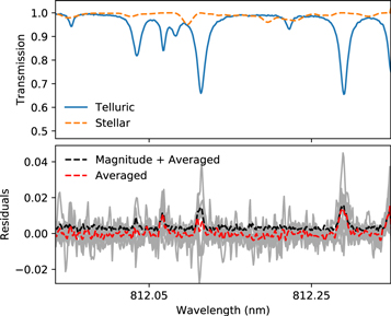
Figure 9. Top: stellar model in orange and median of extracted telluric spectra in blue from group 2; bottom: residuals from the fit in gray, with the average shown in red and the average of their magnitudes shown in black. The residuals shown are from taking the telluric-corrected solar spectra and subtracting off the best-fit solar spline model so that they are centered at zero.
Download figure:
Standard image High-resolution image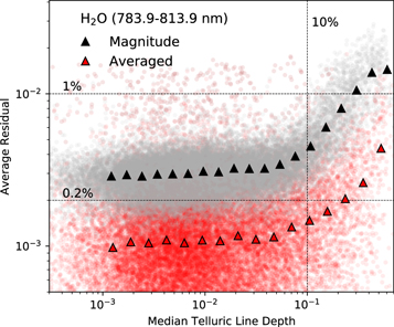
Figure 10. Water vapor average residual vs. median telluric line depth for spectra in group 2. Here a telluric depth of 1 corresponds to a saturated line. The residual array before averaging is defined to be the difference of each telluric-removed solar spectrum and the spline model. The gray points indicate values for which the absolute value was taken of the residual array before averaging, while for the red points the absolute value was taken after averaging. The corresponding triangles show the averages of the data in adjacent bins.
Download figure:
Standard image High-resolution imageMost of the residuals in Figures 9 and 10 are due to not accounting for differences in the line shapes due to changing atmospheric conditions. A possible improvement could be to address this by parameterizing the atmospheric changes in time and modifying the telluric lines by utilizing the HITRAN parameters that describe these pressure and temperature line shape dependencies. Alternatively, a more empirical approach could be adopted, such as what was done in Leet et al. (2019) or in the Wobble code developed by Bedell et al. (2019). Wobble defines the telluric model by three principle components that are linearly combined; the measured flux in each spectral pixel value for each principle component spectrum is solved for directly. While Wobble would not work with solar data owing to the small velocity shifts between the telluric and solar spectra, a physically motivated set of principle components could be used to fit the residuals from our model as was suggested by Artigau et al. (2014), who also developed a principle-component-based empirical telluric fitting algorithm. More investigation would need to be done to validate the usefulness of combining these two methods.
Nevertheless, the telluric modeling code used in this work produces excellent results, and the model may work well farther into the NIR, where many Doppler precision spectrographs targeting K and M dwarfs are being operated in order to capture higher stellar line densities and fluxes. In particular, it avoids propagating any potential errors from line list databases that have been previously shown to affect atmospheric fits in the NIR (Bean et al. 2010; Rudolf et al. 2016), and the ability to adapt the model to fit the RV of stellar lines simultaneously could ultimately increase the fraction of a spectrum that can be used in the RV extraction process, which in the J band can be as high as 55% of the region (Reiners et al. 2010). With a larger barycentric velocity, this could be done for stellar targets without needing as extreme a range in air-mass measurements as was required for the work presented here. The quick evaluation of this analytical model would also make up for the slow convolution step that would need to be added for fitting lower-resolution data.
5.5. Microtelluric Lines
The impact of microtelluric water vapor lines (lines having lower than ∼1% depth relative to the continuum) is a growing concern to the field of high-precision RV measurements that is pushing for the detection of terrestrial-sized exoplanets. Several studies have shown that microtelluric lines, which are not visible after being convolved with an RV spectrograph’s instrument profile, can skew RV measurements and be a large component of a survey’s final error budget (Artigau et al. 2014; Cunha et al. 2014; Halverson et al. 2016; Plavchan et al. 2018).
We point out that this telluric data set would be ideal for studying the temporal variations of microtelluric line shapes since we are able to detect lines of depth 0.5%–1% compared to the continuum and binning multiple spectra in time or with similar air mass would help reduce the noise in the data to be able to study even weaker lines. We show a demonstration of two adjacent microtelluric lines in Figure 11, one due to molecular oxygen absorption and another due to water vapor absorption, and show that these lines are clearly resolved in the average of 13 final telluric spectra. The water vapor line is weaker than our limit on lines included to be individually fit; however, the uniform shift applied to these lines that was largely determined by the stronger features in the region did a good job aligning our model for the weaker telluric feature. Including these microtelluric lines in the telluric model, as we do here, while solving for the RV of the star may alleviate the impact they have on the RV estimates. This should be confirmed in future work.
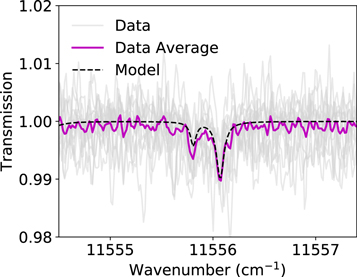
Figure 11. Demonstration of microtelluric lines in the raw data. Here 13 telluric spectra are shown in gray, with their average plotted in magenta and the telluric model in black. The two observed lines are an oxygen feature (left) and a water vapor feature (right) located in an NIR telluric window.
Download figure:
Standard image High-resolution image6. Conclusions
High-resolution spectra of the Sun are important for many astrophysical studies, including the study of stellar activity on Doppler spectroscopy, deriving the abundances of other stars, and understanding solar physics processes. High-resolution spectra in which the individual solar lines are purely resolved are difficult to obtain from space, and ground-based observations are plagued by telluric absorption features that move relative to the solar lines by a maximum of about a kilometer per second, which is not large enough for the stellar and telluric features to dissociate. Therefore, many of the stellar features overlapping telluric lines remain unreliable for analyses in high-resolution solar spectra. Furthermore, the high S/N and high resolution of the telluric lines in FTS solar spectra also make them a useful data set for studying microtelluric lines, which are a poorly studied component in the error budget of next-generation precision spectroscopy instruments.
In this work we presented the telluric-corrected IAG solar flux atlas derived from observations taken in 2015 and 2016 in Göttingen, Germany. We leverage the spread in air mass and Sun–Earth velocity to distinguish between spectral features that are either telluric or solar in origin and utilize a semiempirical telluric model to separate the telluric lines from the solar data. We make available the final telluric-corrected solar spectrum online and additionally save the telluric spectra for possible use in studies such as investigating microtelluric lines or validating various atmospheric models.
We find that our simplified telluric model works well and that the residuals remain below 1% for telluric lines with less than 10% depth with respect to the continuum, with the average residual of these lines being around 0.1%. The addition of more molecular species would be possible for future work to extend this data reduction to the NIR portion of the IAG solar spectral data.
The authors would like to thank the anonymous referee for their comments that improved this manuscript. The authors also thank Dr. Iouli Gordon for his constructive comments on this work and the organizers of the 2019 Telluric Hack Week for hosting a nice week of talks and discussion that led to some of the methods incorporated into our final telluric model. This material is based on work by A.D.B. supported by the National Science Foundation Graduate Research Fellowship under grant No. DGE-1321851.
Appendix A: Justification of the Telluric Model
In defining our telluric model, we choose to fit each telluric line (in units of absorbance) as a simple Lorentz profile initiated with line parameters from the HITRAN database that are then individually optimized. The HITRAN line lists are extensively complete for O2 and H2O, which we model here, making it a reliable starting point for our model. We chose to avoid radiative transfer modeling of Earth’s atmosphere and instead use this semiempirical approach in order to avoid propagating any errors in the line parameter database to our model, with the added benefit of reduced computation times that enabled us to simultaneously fit multiple spectra at once. This allowed the model to leverage the different effects air mass and RV have on the solar and telluric components of the spectra, which is crucial since the maximal range in solar RV (∼±0.7 km s−1) does not result in a separation of the two sources of spectral lines we ultimately wish to dissociate. Limiting the line shapes to a physically motivated functional form and placing these only where known atmospheric features exist is also useful to restrict the model to avoid overfitting telluric residuals. In defining our telluric model this way, we are effectively simplifying the atmosphere to one constant temperature and pressure for all atmospheric heights.
We find that this simplification and fitting each line individually as a Lorentz function are good approximations and allow us to achieve residuals consistently below 2% even for some saturated water vapor regions. We experimented with more complex line shapes, including Voigt, but found that for the water lines the Lorenztian profile was a sufficient description of the line shape given our data.11 This can be seen in Figure 12, where we show a nearly isolated water vapor transition with the best-fit solar spectrum removed. Comparing this strong line (50% deep) to the best-fit Lorentz model produces residuals near the noise in the data, with only an S-shaped structure nearing 1% in magnitude in the core of the line. This was expected since the water vapor lines are formed at lower altitudes and therefore are primarily pressure broadened (Hedges & Madhusudhan 2016). This is not necessarily true of oxygen since it extends into the upper atmosphere and therefore has a larger Doppler broadening component, making a Voigt profile a better approximation. The resulting S-shaped residuals from the simplification of the line shapes for both species vary at a frequency that is typically too high for our stellar spline model to capture (see Section 3.1.4) and do not correlate with the solar RV. Therefore, we can simply replace regions overlapping dense telluric absorption with the spline fit to remove the majority of these telluric residuals. Because we perform our fits on 11 groupings of data, any telluric residuals captured by our spline model should vary in strength between the 11 best-fit stellar models and can therefore still be identified as unreliable.
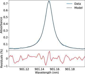
Figure 12. Example isolated water vapor feature along with a best-fit Lorentz profile.
Download figure:
Standard image High-resolution imageAppendix B: Basis Splines
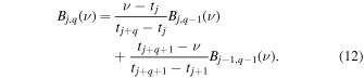
The basis splines,  , are calculated internally by the BSpline function and are defined recursively as follows using tj as the knot locations that match the units of ν:

Appendix C: Zero-point Offset from Telluric Lines
We also investigated using the oxygen lines for the purpose of finding an accurate wavelength scale but found that uncertainties in the fitted line centers and the δair parameters that determine each line’s pressure-induced shift made it difficult to calculate a more accurate estimate of a zero offset velocity than can be achieved using the iodine template. Fitting a line to the line-center shifts found in this work versus the HITRAN δair parameters allows us to solve for a zero offset velocity that would shift the fitted line to cross the origin (i.e., an extrapolated δair value of zero induces no measured line shift). Doing this, we found the offset to be 0.005 ± 0.004 cm−1 using all oxygen lines for which our measured line centers had uncertainties of less than 6 × 10⁻⁴ as determined by the standard deviation of the values found in our 11 fits. For δair we assumed a uniform uncertainty of 5 × 10⁻⁵, which reflects what is reported in Robichaud et al. (2008). We note that the evaluated zero-point offset depends on the source of the measurement and the isotopologue number, which is likely due to offsets in δair, which are calculated in reference to the lines of another species, typically either iodine or carbon monoxide, and which species is chosen will offset the measured value. While the water vapor lines have higher δair uncertainties (Jacquemart et al. 2005), there are also more data points, and together they provide an estimate of 0.0063 ± 0.0020 cm−1. Both of these estimates are slightly sensitive to the errors assumed for δair but remain consistent with the zero offset velocity determined using the iodine lines.
Footnotes
- 3
- 4
- 5
We use γair from HITRAN for both molecules.
- 6
- 7
We found best behavior using the sequential least-squares programming algorithm in the scipy.optimize.minimization function.
- 8
The strong lines have depths greater than around 5% in linear normalized flux on average.
- 9
We use an arbitrary definition for what constitutes “dense” that involves summing the telluric model and comparing it to a predetermined threshold value.
- 10
- 11
Although the water vapor line shapes are not necessarily symmetric and will change in time owing to different atmospheric conditions along the line of sight, our fit optimizes an average line shape for the different observations, and ultimately these residuals are reduced through averaging the spectra together.