Abstract
White dwarfs (WD) with main-sequence (MS) companions are crucial probes of stellar evolution. However, due to the significant difference in their luminosities, the WD is often outshined by the MS star. The aim of this work is to find hidden companions in Gaia’s sample of WD candidates. Our methodology involves applying an unsupervised machine learning algorithm for dimensionality reduction and clustering, known as a self-organizing map (SOM), to Gaia BP/RP (XP) spectra. This strategy allows us to naturally separate WDMS binaries from single WDs from the detection of subtle red flux excesses in the XP spectra that are indicative of low-mass MS companions. We validate our approach using confirmed WDMS binaries from the Sloan Digital Sky Survey and LAMOST surveys, achieving a precision of ∼90%. We demonstrated that the luminosity of the faint companions in the missed systems is ∼50 times lower than that of their WD primaries. Applying our SOM to 90,667 sources, we identify 993 WDMS candidates, 506 of which have not been previously reported in the literature. If confirmed, our sample will increase the known WDMS binaries by 20%. Additionally, we use the Virtual Observatory Spectral Energy Distribution Analyzer tool to refine and parameterize a “golden sample” of 136 WDMS binaries through multiwavelength photometry and a two-body spectral energy distribution fitting. These high-confidence WDMS binaries are composed of low-mass WDs (∼0.42M⊙), with cool MS companions (∼2800 K). Finally, 13 systems exhibit periodic variability consistent with eclipsing binaries, making them prime targets for further follow-up observations.
Original content from this work may be used under the terms of the Creative Commons Attribution 4.0 licence. Any further distribution of this work must maintain attribution to the author(s) and the title of the work, journal citation and DOI.
1. Introduction
It is well established that the binary fraction of stars is highly dependent on the stellar mass, ranging from 30% for M-type stars (J. G. Winters et al. 2019) to 70% for O- and B-type stars (H. Sana et al. 2014; M. Moe & R. Di Stefano 2017), with a mean incidence of 50% for solar-type stars (D. Raghavan et al. 2010).
The more massive star in the pair will evolve faster and, if it is a low-to-intermediate-mass star (≲8 ), it will eventually become a white dwarf (WD, I. J. Iben et al. 1997) forming a WD plus main-sequence (MS) star binary (hereafter, WDMS). Given the very predictable cooling age of the WDs, WDMS binary pairs are excellent cosmic clocks that have been used to study fundamental astrophysical parameterizations such as the age–metallicity relation (A. Rebassa-Mansergas et al. 2021), the initial-to-final mass (J. K. Zhao et al. 2012), and the mass–radius relation (R. Raddi et al. 2025).
Different outcomes are expected for the WDMS binary depending on the orbital separation. In wide orbit pairs, the MS companion evolves independently eventually leading to the formation of a WD–WD binary. Conversely, close WDMSs are susceptible to undergo mass transfer episodes, potentially leading to cataclysmic variables (CVs; S. G. Parsons et al. 2013; Y. Sun et al. 2021), Novae, Symbiotic, and Type Ia Supernovae (SNe; B. Wang & Z. Han 2012), essential tools in cosmological and stellar evolution studies (B. Leibundgut & M. Sullivan 2018).
The most extensive samples of WDMS to date are those obtained by the Sloan Digital Sky Survey (SDSS, see, e.g., A. Rebassa-Mansergas et al. 2016) and the Large Sky Area Multi-Object Fiber Spectroscopic Telescope (LAMOST, see, e.g., J.-J. Ren et al. 2018) with a total of 4100 WDMSs. However, both surveys exhibit certain observational biases against cool WDMSs, resulting in an apparent absence of systems with Teff < 10,000 K.
Several studies have demonstrated the feasibility of automatically identifying WDMS binaries using machine learning techniques with promising accuracy (around 80% using random forest; see D. Echeverry et al. 2022), and successfully detecting candidates in open clusters with support vector machines (SVM; S. M. Grondin et al. 2024). M. L. Kao et al. (2024) in particular, identified an isolated group of 1096 WDMS candidates by using a uniform manifold approximation and projection (UMAP) through the largest white dwarf catalog available to date. Recently, we have used self-organizing maps (SOMs; T. Kohonen 1982), an unsupervised neural network-based algorithm to find polluted WD candidates based on Gaia XP spectra (X. Pérez-Couto et al. 2024).
In this work, we will use a similar methodology to that used in X. Pérez-Couto et al. (2024) to identify MS companions in WD spectra from the catalog of N. P. Gentile Fusillo et al. (2021). This catalog is built using color–magnitude and astrometric cuts to prioritize single WDs. Therefore, any secondary companion to a WD in the sample is expected to be a low-mass, late-type M dwarf or even a brown dwarf, as its presence is not expected to significantly affect the photometry or astrometry of the WD.
The paper is organized as follows: in Section 2, we describe the data used and the SOM learning process, in Section 3 we apply the method to the data and discuss the results. Finally, in Section 4 we summarize our main findings and present the conclusions of the paper.
2. Methodology
The Gaia Mission (Gaia Collaboration et al. 2023) has provided, in its Third Data Release (DR3), high-quality astrometric data and photometry from the Blue (BP) and Red Photometers (RP) for 1460 million sources of our Galaxy. This extensive data set has been instrumental in identifying new WDMSs by using the Gaia G, GBP, and GRP color–magnitude diagram (CMD) and Virtual Observatory (VO) tools. In particular, the Virtual Observatory Spectral Energy Distribution Analyzer (VOSA;7 A. Bayo et al. 2008) allowed A. Rebassa-Mansergas et al. (2021) to find 97 new WDMS and parameterize their stellar properties.
In addition to the BP/RP photometry, Gaia published low-resolution (R ≈ 70) BP/RP spectra (hereafter, XP spectra) for about 220 million sources (F. De Angeli et al. 2023). Instead of flux units per wavelength unit, each XP spectrum is given as an array of 110 coefficients of a series of Hermite basis functions (55 for BP and 55 for RP). Given the infeasibility of visually inspecting such an extensive data set, numerous studies have employed machine learning (ML) algorithms to mine the data in the search and classification of WD (E. M. García-Zamora et al. 2023; M. L. Kao et al. 2024; X. Pérez-Couto et al. 2024; O. Vincent et al. 2024; E. M. García Zamora et al. 2025).
SOMs (T. Kohonen 1982) is an unsupervised neural network-based algorithm that combines dimensionality reduction—to project the XP coefficients in a two-dimensional grid map—and cluster—to group similar elements together in the same neuron. The power of this dual technique demonstrates that SOMs are a useful artificial intelligence tool for object classification in various fields of astrophysics (see, e.g., S. Torres et al. 1998; A. Naim et al. 2009; D. Ordoñe-Blanco et al. 2010; J. E. Geach 2012; M. Way & C. Klose 2012; D. Fustes et al. 2013a, 2013b; K. M. Carrasco & R. J. Brunner 2014; C. Dafonte et al. 2018; M.A. Álvarez et al. 2022; X. Pérez-Couto et al. 2024).
2.1. Input Data
The initial sample is based on the N. P. Gentile Fusillo et al. (2021) catalog, where a large sample of WD candidates is selected first by imposing the following cut in the Gaia CMD:

a parallax_over_error > 1 and several additional quality cuts to discard bad astrometric solutions up to a final sample size of 1.3 million sources.
This color cut is indeed not the most effective way of identifying a large number of WDMS binaries, as it excludes WDs situated in the CMD between the WD locus and the MS branch—a region above which approximately 90% of WDMS binaries are expected to be found, according to recent population synthesis simulations (A. Rebassa-Mansergas et al. 2021; A. Santos-García et al. 2025). Nevertheless, we adopt this color cut in the present study, which specifically focuses on the WD region. This approach ensures that any detected companion has low emission, as the WD dominates, making very-low-mass companions, such as M stars or brown dwarfs, the most likely candidates.
Some astrometric cuts used in the N. P. Gentile Fusillo et al. (2021) catalog such as the Renormalized Unit Weight Error (RUWE) < 1.1, ipd_gof_harmonic_amplitude < 1, or astrometric_excess_noise_sig <2 efficiently clean the sample from the majority of astrometric contaminants (among them, many unresolved binaries) (V. Belokurov et al. 2020). This, in conjunction with the fact that they are unresolved despite their proximity, makes any WDMS binary found in their catalog a very close binary.
In N. P. Gentile Fusillo et al. (2021), the authors computed a probability of an object being a WD (PWD). This probability is determined using a reference data set of 22,998 spectroscopically confirmed WDs and 7124 contaminants identified through visual inspection in the SDSS. These data sets are modeled as normalized 2D Gaussian distributions, producing distinct density maps for WDs and contaminants. The PWD for each candidate is calculated by integrating its CMD Gaussian representation with a map formed by taking the ratio of the WD density map to the combined density of both WDs and contaminants.
The definition of contaminant used in N. P. Gentile Fusillo et al. (2021) included WDMS binaries, and hence a probability filter of, for instance, PWD > 0.9, would exclude the majority of contaminants such as QSOs or galaxies, but also most of the WDMS we aim to discover. For this reason, we will not use the PWD in the following.
In contrast, we only consider as contaminants those sources with the SDSS spectral classes “QSO,” “GALAXY,” and “STAR.” The “Unreli” (for unreliable) and “UNKN” (for unknown) sources in the Gaia-SDSS sample of N. P. Gentile Fusillo et al. (2021) were discarded from the sample since we are not confident to confirm if they are WDs or contaminants. This leaves us with 26, 423 SDSS confirmed WDs (either single or binary sources) and 4588 contaminants.
Subsequently, we use a parallax ( ) over error (
 ) (or
) (or  ) > 10 that will ensure a more precise Gabs, and therefore a more reliable location in the CMD. Additionally, we have included these additional filters to ensure the quality of XP spectra:
(i) visibility_periods_used > 10, where each visibility period is a group of observations separated from the next by at least 4 days, so that only those sources that were astrometrically well observed are retained (L. Lindegren et al. 2018).
(ii) (phot_bp_n_obs > 10) and (phot_rp_n_obs > 10), refer to the minimum number of CCD transits for BP and RP spectra, respectively, following the recommendations set forth by R. Andrae et al. (2023) to ensure an adequate signal-to-noise ratio (S/N) for subsequent spectral analysis.
(iii) ∣phot_bp_rp_excess_factor_corrected∣ < 5 x sigma_excess_factor ensures that the photometry of GBP, GRP, and G is consistent and free from contamination from external sources in the same field of view, as elucidated by M. Riello et al. (2021).
We obtained the Gaia XP spectra for this sample using the DataLink Gaia tool (available at https://www.cosmos.esa.int/web/gaia-users/archive/datalink-products) through the astroquery Python package (A. Ginsburg et al. 2019).
Finally, an S/N > 10 filter was applied through the coefficients. The S/N for both BP and RP spectra was calculated by taking the ratio between the  norm of the BP (RP) array of coefficients and the
  norm of the array of BP (RP) coefficient uncertainties. As a result, we obtained an initial sample for our study comprising a total of 90,667 sources.
To roughly estimate the contaminant ratio in our sample, as well as the effectiveness of the  filter in discarding them, we show in Figure 1(b) the Gaia CMD with the SDSS confirmed WDs and contaminants that meet the above filters in blue and red, respectively. However, in the CMD of the left (Figure 1(a)) we relax the parallax-over-error filter up to the original value in N. P. Gentile Fusillo et al. (2021):
  , while in the right (Figure 1(b)) we show the resulting CMD for
  .
.
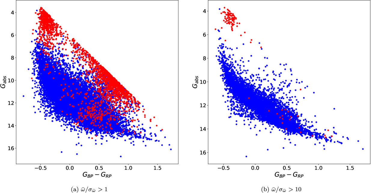
Figure 1. SDSS confirmed WDs (in blue) vs. contaminant (in red) CMD with  (left) and
  (right).
Download figure:
Standard image High-resolution imageAs illustrated in Figure 1, the image on the right is visibly more pristine and devoid of contaminants. Indeed, the contaminant fraction has been reduced from 7.5% (2074 contaminants) to 0.9% (112 contaminants), indicating that the input sample of the SOM is unlikely to contain a contamination level greater than 1%.
2.1.1. Reference Catalogs
Despite the unsupervised nature of the classification process, which does not rely on a training data set, spectroscopically confirmed WDMS spectra are required as a reference to label the final clusters. As a baseline, we rely on the Montreal White Dwarf Database8 (MWDD), which is so far the most complete catalog of WDs based on more than 200 references from the literature (P. Dufour et al. 2017), containing information about each WD such as its spectral type or binarity. As of 2025 January 30, it contains information for 144,800 WDs. Most of them also belong to the catalog of O. Vincent et al. (2024), which is an automatic classification of Gaia DR3 XP spectra based on gradient-boosted decision trees. Despite the great performance shown by their method, their classification is still based on Gaia low-resolution spectra, and thus it is a catalog of WD candidates instead of confirmed WDs.
Therefore, we decided to ignore sources with only low-resolution spectra in order to keep our reference sample of confirmed WDs as clean as possible. To this end, we discarded those sources included in the O. Vincent et al. (2024) catalog if they had only one available optical spectrum. For the rest of the MWDD, we used all the sources with at least one available spectrum and a confirmed spectral type. We did not include sources with subdwarf (sdO, sdB, …) spectra.
From this set, we selected as WDMS sources those with the “WDMS” binarity flag, resulting in 2849 sources. We also included some sources from the MWDD without a positive binarity flag but with a spectral type containing one of the following strings: “+M,” “+dM,” “+K,” “+G,” or “+F,” which indicate the presence of an MS companion in the source’s spectra. This resulted in an updated WDMS count of 3246, of which 377 have XP spectra available and that passed the filters described in Section 2.1.
We also cross-matched this MWDD WDMS sample with the largest WDMS catalogs up to date: the SDSS DR12 WDMS spectroscopic catalog (A. Rebassa-Mansergas et al. 2010, 2012, 2013, 2016) and the LAMOST DR5 catalog (J. J. Ren et al. 2014; J.-J. Ren et al. 2018). As a result, 14 SDSS WDMS that are not classified by the MWDD as binaries have been added, as well as 19 LAMOST WDMS. This resulted in a final WDMS sample of 406 sources (4 sources were duplicated) that will be used as a reference in the labeling process of the SOM.
The remaining MWDD sources that are not included in the WDMS binary sample and that do not correspond to any other type of binarity (i.e., those with an empty binarity field in the MWDD and a spectral type without a “+” sign) are designated as single WD sources (13,426 sources), and the remaining sources in our initial sample (76,835 sources) are considered candidates in the following.
2.2. Self-organizing Maps
While most unsupervised machine learning techniques are either utilized for dimensionality reduction (e.g., t-SNE, UMAP) or clustering (e.g., K-means, DBSCAN), SOMs integrate both applications within a single neural network-based algorithm. Indeed, given a high-dimensional nonlinear data set (in our case, constructed from arrays of 110 coefficients per spectrum), the SOM projects each element on a two-dimensional map, where analogous elements are assigned to the same neuron. Moreover, neurons with similar subpopulations are also grouped in the map, while very different subpopulations are highly distanced. This results in preserving the topology order, allowing for the recognition of patterns in the data. Furthermore, the clustering of neurons into closed groups allows the accurate delineation and classification of these populations.
Once the dimensions of the map M × N have been established, the learning process starts with a random initialization of the weight, wm,n, of each neuron, zm,n. Each wm,n is a random array of 110 elements. After that, the first iteration takes each XP spectrum, xi, and looks for the winner neuron or best matching unit (BMU), zm,n, by minimizing the distance (for example, the Euclidean distance) between xi and wm,n is the minimum possible among all weights. Subsequently, an iterative process updates the weights at a given learning rate (h0) that decreases over time, and following a neighborhood function that ensures the preservation of the topology. This neighborhood function (usually a Gaussian) is governed by a parameter ν that defines the initial spread of the neighborhood of each neuron.
The learning process ends after a maximum number of iterations,  , or when the weights do not change significantly (T. Kohonen 1982). Finally, each neuron (and thus the candidates that fell into it) receives the label corresponding to the majority class, taking as a reference the sources with a confirmed classification.
The SOM implementation used in this work is the Python MiniSom 9 library for its ease of use and flexibility in hyperparameter configuration (G. Vettigli 2018). In the following, we will assume a squared map, M = N (for simplicity and because the total number of neurons is much more crucial than their distribution)
Subsequently, to choose the best hyperparameters for the SOM (namely, the map size N2, ν, h0, and  ) we implemented a grid search process, assuming for simplicity a squared map (N = M) with N ∈ {5, 6, 7, 8};
 ![$\nu \in \left[0.5,1.5\right]$](https://content.cld.iop.org/journals/0004-637X/988/1/51/revision1/apjaddfd7ieqn14.gif) and
and ![${h}_{0}\in \left[0.1,1.0\right]$](https://content.cld.iop.org/journals/0004-637X/988/1/51/revision1/apjaddfd7ieqn15.gif) , both in steps of 0.1; and the number of iterations nmax ∈ {100, 500, 1000, 5000, 10,000}.
, both in steps of 0.1; and the number of iterations nmax ∈ {100, 500, 1000, 5000, 10,000}.
We built the cost function, f = f(N, ν, h0, nmax) to minimize as a composition of three different metrics: the quantization error (QE), the topographic error (TE), and the F1-score.
The QE is defined as the mean distance between each element xi and their BMU and indicates how well the SOM represents the input data (T. Kohonen 1982), while the TE, quantifies the fraction of input samples for which the first and second BMU neurons were not placed adjacent in the map. That is, the TE is a measure of how well the SOM preserved the topology (K. Kiviluoto 1996). Both QE and TE are computed with Equations (2) and (3):


where (xi) = 1 if the first BMU(xi) and the second BMU(xi) are not adjacent, and
(xi) = 0 otherwise.
On the other hand, the F1-score is defined as the harmonic mean of the precision10 and the recall11 of the classification, and calculated with Equation (4):

Therefore, to achieve a good SOM classification, we must aim to minimize QE and TE, while maximizing the F1-score. To do this, we expressed  , where the symbol “
  ” means that those three quantities have been previously scaled with the min–max normalization, and look for the minimum in the parameter space shown above. As a result, we found the global minimum with a map size of 8 × 8 neurons, ν = 1.4, h0 = 0.4, and 5000 maximum iterations.
It is important to recognize that the effectiveness of this approach, like other distance-based algorithms, is strongly tied to the scale of the features involved (here, the XP coefficients). To remove distance-dependent effects and focus the SOM training on spectral morphology rather than flux amplitude, we normalized each XP coefficient vector by its  norm (
 ), which linearly correlates with the G-mean flux (FG) of the source, as shown in Figure 2. This procedure has already been used in F. De Angeli et al. (2023) to optimize the set of basis functions used to represent the XP spectra.
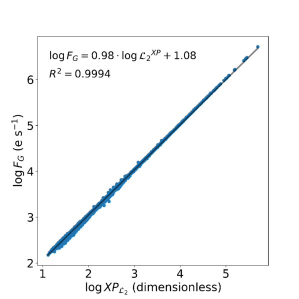
Figure 2. Linear relation between  and FG as calculated with the 90,667 sources used in this work.
Download figure:
Standard image High-resolution image3. Results
3.1. Spectral Classification
We incorporated the 90,667 sources in the form of normalized XP data into the SOM with the hyperparameters defined in Section 2.2. The resulting map is shown in Figure 3, where confirmed WDMS binaries are plotted in orange, single WDs are plotted in blue, and candidates are invisible to enhance visualization.
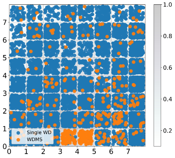
Figure 3. SOM map with our sample of 90,667 sources. WDs with a confirmed MS companion appear in orange, single WDs appear in blue, and candidates are invisible to enhance visualization.
Download figure:
Standard image High-resolution imageAs illustrated, some confirmed WDMS binaries share the same neurons as single WDs due to their XP composite spectra being entirely dominated by the WD component. Notwithstanding that, two neurons (z3,0 and z4,0) are clearly dominated by WDMS binaries. Indeed, among the WDs fallen in neuron z3,0, 85% are confirmed WDMS binaries; a percentage that is increased up to 92% in neuron z4,0. Therefore, we labeled them as WDMS neurons. The other 23 neurons (having a percentage of WDMS <50%) are considered in the following as single WD neurons.
Using this labeling procedure, we can compute a confusion matrix (see Figure 4), as well as precision and recall metrics (see Table 1) to validate our methodology. The confusion matrix, C, has as rows the true labels (that is, those used as a reference, here MWDD combined with SDSS and LAMOST) and as columns the predicted labels (those assigned after the SOM clustering plus the labeling procedure described above). In this way, each cell Ci,j contains the number of sources of the i class, classified by our SOM as belonging to the j class.
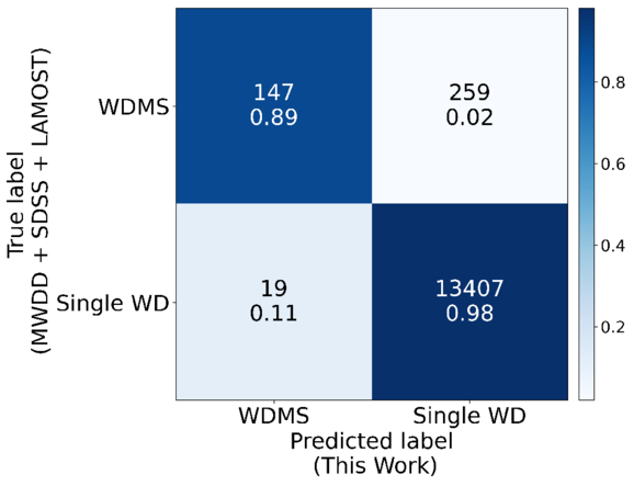
Figure 4. Confusion matrix of the binary WDMS–Single WD SOM classification.
Download figure:
Standard image High-resolution imageTable 1. Precision and Recall Metrics for WDMS–single WD Classification
| Class | Precision | Recall | F1-score |
|---|---|---|---|
| WDMS | 0.89 | 0.36 | 0.51 |
| Single WD | 0.98 | 1.00 | 0.99 |
Download table as: ASCIITypeset image
In Figure 4 we show the confusion matrix with the numbers described above in each cell, and below them the same number normalized by columns, which is equivalent to the precision. In addition to that, in Table 1 the precision, recall, and F1-score for each class are summarized.
As can be seen, our classification shows excellent precision (∼90%) in identifying WDMS binaries. However, its low recall (only a third of the WDMS binaries are classified as such) suggests that they are systems where the WD flux overwhelms that of the cool companion.
Although both z3,0 and z4,0 contain WDMS binaries, they are different neurons, which, based on the conservation of the topology order, suggests that there is some difference between their populations. Indeed, the median, 25th, and 75th percentile of the GBP − GRP color of the input samples in the z3,0 neuron (hereafter, the cool WDMS neuron) is  mag, while for the z4,0 neuron (hereafter, the hot WDMS neuron) it is
  mag. Moreover, by using the Teff computed in N. P. Gentile Fusillo et al. (2021) from the G, GBP, and GRP photometry assuming H-rich atmospheres, we obtained a corresponding median Teff of
  K for the cool WDMS neuron and
  K.
K.
In general, the distribution of GBP − GRP color across the two axes of the SOM is not expected to be irregular, since color and, correlatively, the Teff are highly dependent on the spectral shape. Indeed, if we plot the GBP − GRP color of the 90,667 sources present in the SOM, we see a smooth, nonlinear gradient with the cooler sources on the left and the bluer ones on the right, as shown in Figure 5.
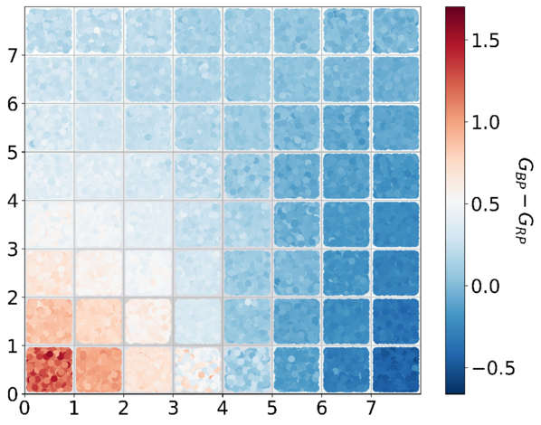
Figure 5. The SOM map displays the GBP − GRP color of the 90,667 sources. A smooth, nonlinear GBP − GRP color gradient is shown.
Download figure:
Standard image High-resolution imageThere are 993 sources classified as WDMS binaries (525 in the cool WDMS neuron and 468 in the hotter one), of which 846 (85%) have not yet been classified as WDMS binaries in the MWDD, SDSS, or LAMOST catalogs. These sources are therefore new WDMS binary candidates.
In Figures 6(a) and (b) we show the normalized median externally calibrated spectra of the cool and hot WDMS neurons, obtained with the GaiaXPy12 library. For comparison, we also show in green the normalized median spectra of single WD neurons, with a median GBP − GRP color similar to that of the WDMS neurons, so that the continuum can be compared.
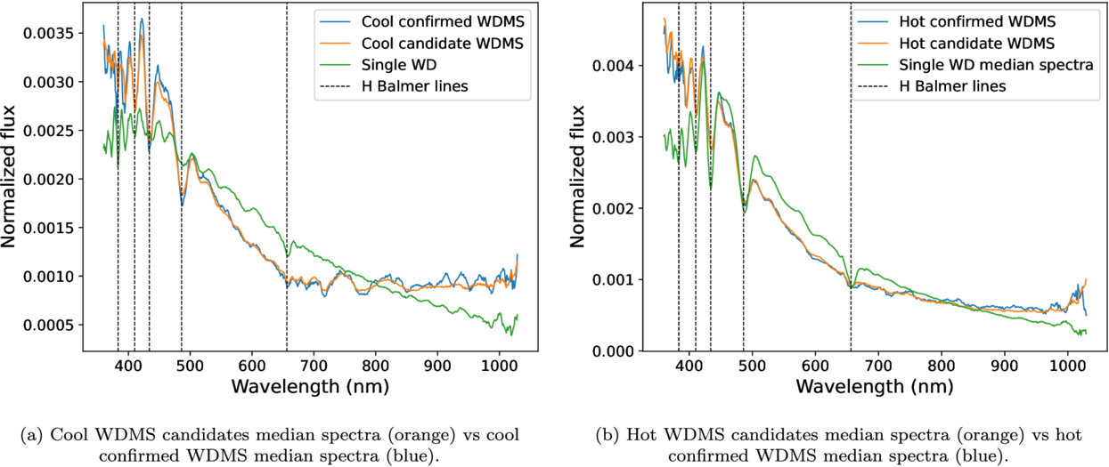
Figure 6. Comparison between the normalized median spectra of the confirmed WDMS (blue) and that of the candidates (orange) for both the cool and hot WDMS neurons. The median spectra of a single WD neuron with comparable GBP − GRP color is included (green) so that the red flux excess can be seen.
Download figure:
Standard image High-resolution imageAs can be seen in Figures 6(a) and (b), both cool and hot WDMS median spectra show a clear red flux excess with respect to the single WD continuum, thus indicating the presence of an optical, late-type stellar companion in their composite spectra.
There exists the possibility that a red flux excess is due to the emission from a disk around the WD (C. S. Brinkworth et al. 2012; J. Farihi et al. 2012; C. Melis et al. 2012; S. Xu & M. Jura 2012; S. Hartmann et al. 2016; L. K. Rogers et al. 2024; A. Swan et al. 2024). We explored the possibility that the map mistook cool companions for hot disks. We put the sample of 33 WDs with disks recorded so far in the MWDD and with available XP spectra and found that none of them fell into the binary neurons. While this does not fully exclude the possibility that some of our WDMS pairs are WDs with disks, we take as a working hypothesis that those red flux excesses are associated with MS stars due to the low number of disks observed surrounding WDs (about 1%–3%; T. G. Wilson et al. 2019).
Furthermore, to assess the reliability of our morphological clustering, we have compared the median spectra of the 455 (391) cool (hot) WDMS binary candidates with that of the 70 (77) cool (hot) confirmed WDMS binaries in each neuron. As shown in the same Figure 6, in both cases the median spectra of the confirmed and candidate WDMS binaries overlap almost perfectly.
3.2. WDMS Eclipsing Binary Candidates
It is of great interest to look for variability indicators in our 993 sources’ sample, since it seems reasonable to expect that the orbit of some of those systems could be aligned with the line-of-sight of Gaia, turning them into eclipsing binaries.
Indeed, 101 (10%) of our 993 WDMS candidates appear as variable sources in the Gaia Archive (phot_variable_flag = “VARIABLE”) so it is tempting to link that variability with the binarity clues found in their XP spectra, either because they may be CVs or eclipsing binaries. This fact is particularly enlightening given that merely 1651 sources (2%) are found to be variable within those sources in the single WD neurons.
To shed more light on this issue, we cross-matched our sample with the all-sky Gaia DR3 Eclipsing Binary catalog (gaiadr3.vari_eclipsing_binary table, see N. Mowlavi et al. 2023) that contains 2,184,477 eclipsing binary candidates obtained from G-band light curves cleaned and modeled to find their orbital period.
As a result, we found that 13 (1%) of our WDMS binary candidates appear in that catalog. In contrast, 100 times fewer eclipsing binary candidates are found in the single WD neurons: only 13 sources, or 0.01%. The orbital periods (P) of our 13 WDMS eclipsing binary sample are available, ranging from ∼0.2 to ∼1.5 days, with a median of 0.5 days. This finding suggests that their orbits are particularly close.
3.3. Stellar Parameterization with VOSA
In order to validate our sample of WDMS candidates with external data and to estimate their astrophysical parameters, we used VOSA. This VO tool enables us to gather photometric data from major multiwavelength astronomical surveys and to compile these data into an observational SED (A. Bayo et al. 2008).
This SED is subsequently used to fit the stellar parameters of the source by using any theoretical model publicly available in the literature. Furthermore, VOSA enables the implementation of a binary fit algorithm, which aims to fit two models to the SED simultaneously: one model for each companion.
To apply VOSA to our WDMS candidates, we used the following input parameters: the Gaia DR3 source ID, equatorial coordinates in J2000.0 (to calculate them from the Gaia J2016.0 epoch, we employed proper motions and parallax information in Gaia, and the astropy library; Astropy Collaboration et al. 2022), geometric distances from the catalog of C. A. L. Bailer-Jones et al. (2021), and the mean visual extinctions Av calculated in N. P. Gentile Fusillo et al. (2021).
As source catalogs for the photometric points we used the GALEX GR6/7 (L. Bianchi et al. 2017) in the UV range; SDSS DR12 (S. Alam et al. 2015), Gaia DR3 (Gaia Collaboration et al. 2023), and Pan-STARRS DR2 (E. A. Magnier et al. 2020) in the optical; and DENIS (N. Epchtein et al. 1994), 2MASS (M. F. Skrutskie et al. 2006), and CatWISE2020 (F. Marocco et al. 2021) for the near-IR (NIR). Furthermore, since we have Gaia XP spectra available for every source, we also incorporated their J-PAS synthetic photometry with GaiaXPy (N. Benitez et al. 2014; P. Montegriffo et al. 2023). All photometry was programmatically retrieved with VOSA, except that from CatWISE2020 and J-PAS since they are not currently included in VOSA, so we loaded them manually.
Once VOSA has obtained the photometric points of each source, it automatically rejects those points bearing bad quality flags in their respective catalogs. An equivalent procedure was applied to our CatWISE2020 photometry by imposing high-quality flags (ccf = 0000 and ab_flag = 00, see F. Marocco et al. 2021 for further details). Moreover, we discarded any point in the overall photometry with a relative error for the flux greater than 20% and retained only those sources with at least a point from 2MASS and CatWISE2020 photometry, to ensure NIR coverage. This last filter is highly conservative and reduces our final sample of WDMS with computed parameters (from 993 to 323 sources). However, we consider it crucial if we want to obtain a reliable SED fit since the low-mass MS companions are expected to have their emission peak in the NIR. Furthermore, by doing so we prevent overfitting issues due to the high number of optical points mainly provided by the J-PAS synthetic photometry.
Subsequently, we fitted the resulting photometry to three distinct types of models: a single-body fit to the BT-Settl-CIFIST model (I. Baraffe et al. 2015; setting 1200 ≤ Teff/K ≤ 7000 and  for MS stars), a single-body fit to the WD Koester model (D. Koester 2010; 5000 ≤ Teff/K ≤ 80,000 and
  ), and a two-body fit using both models simultaneously.
It should be noted that, although the WD Koester model assumes hydrogen-rich (DA) atmospheres, this hypothesis is more than reasonable in our work since our WDMS candidates clearly show Balmer lines, as can be seen in Figure 6.
To assess the quality of a fit, VOSA uses the visual goodness-of-fit (Vgfb), a modified version of the reduced χ2 in which the relative photometric errors are considered to be at least 10%, to prevent any underestimation of the uncertainties. In this way, an SED is considered well-fitted if Vgfb < 10–15. Notwithstanding that, P. K. Nayak et al. (2024) have detected that some SED fittings with low Vgfb are not always satisfactory. Moreover, a preliminary analysis of some fits in this work has shown that a Vgfb < 10 is compatible with a  as high as 100 or 1000. Consequently, we decided to use
 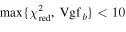 as a more conservative but reliable criterion to define a good quality SED fitting.
From the sample of 323 WDMS binary candidates with available optical and NIR photometry, 137 of them show an excellent fit to the binary WD Koester—BT-Settl SED model, according to the criteria described above. Moreover, none of our sources show a good fit to the single BT-Settl SED, and only one source fitted well to the single WD Koester SED, with a better  and Vgfb than for the binary SED fit, so we discarded it.
As a result, we have obtained a golden sample of 136 high-confidence WDMS binary candidates for which VOSA provides the best-fitted Teff and bolometric flux (Fbol) for each companion.
In Figure 7 we present the calibrated XP spectra of the cool and hot WDMS neuron prototype (i.e., the source most similar to the externally calibrated median spectra) in the left, and their VOSA binary fitted SEDs in the right.
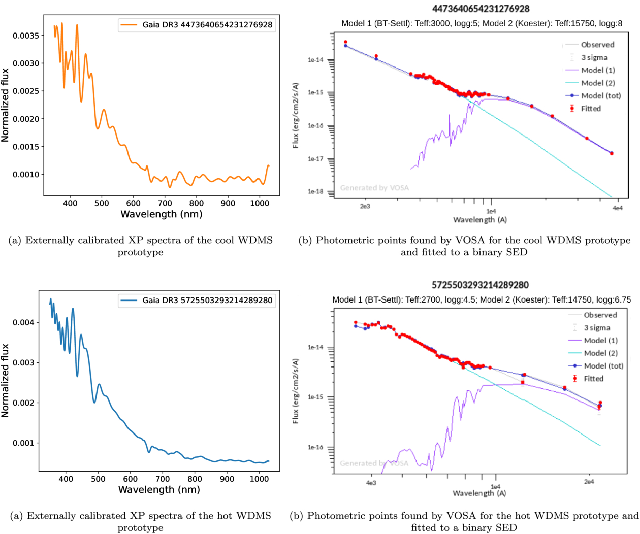
Figure 7. Calibrated Gaia XP spectra and two-body SED fitted for the cool (top) and hot (bottom) prototypes of the WDMS binary candidates.
Download figure:
Standard image High-resolution imageThe final WDMS binary candidates show median, 25th, and 75th Teff percentiles for the WD companion of  K, although there is a slight difference between the median Teff of hot and cool neurons (12,500 K for the cool neuron and 17,250 K for the hotter one). These values are approximately 5000–6000 K higher than those obtained from the Teff calculated in N. P. Gentile Fusillo et al. (2021) assuming a single WD. This discrepancy is most likely due to the fact that they only used the G, GBP, and GRP colors to fit their atmospheric models while we used a significantly larger set of photometric points spanning a wider wavelength range from the UV (where the emission peak in WDs is located) to the NIR.
Regarding the MS companion, the Teff has a median, 25th, and 75th percentile of  K that, when translated to spectral types using the updated tables of M. J. Pecaut & E. E. Mamajek (2013), is equivalent to a median M6V type.
It is worth mentioning that there are nine sources in which the faint companion has Teff ≤ 2250 K, compatible with a brown dwarf (BD) candidate (M. J. Pecaut & E. E. Mamajek 2013; J. D. Kirkpatrick et al. 2021). Further spectroscopic follow-up observations are planned to confirm these objects.
Finally, we leveraged VOSA to fit the 406 confirmed WDMS binaries that were used during the labeling process of the SOM training to a binary SED, using the same models as above (but without the NIR photometry requirement). We found, with  , that the median Lbol ratio (computed as Lbol,MS/Lbol,WD) for the missed WDMS binaries is 0.02, while that of the detected WDMS is 0.13, and their difference is statistically significant (Mann-Whitney U’s test p-value ≈10−14 ⋘ 0.05). This confirms that the WDMS binaries missed by the SOM are those whose WD flux overwhelms that of the cool companion.
3.4. Stellar Masses
In principle, WD masses cannot be directly determined by VOSA, since the SED fitting has not enough sensitivity to  which, furthermore, it has an uncertainty as large as 0.5 dex. Therefore, to compute the WD mass (MWD) we used the evolutionary models of A. Bédard et al. (2020) along with the Teff and Lbol determined in the previous Section 3.3.
In Figure 8 we present the WD evolutionary sequences of A. Bédard et al. (2020) in a Lbol–Teff diagram for different masses (among 0.2M⊙ and 1.3M⊙), assuming a C/O core, He mantle, and a thick H outer layer. Over them, we plotted our 136 golden WDMS binary candidates. Subsequently, we calculated the MWD for each WD by means of a linear interpolation. There are only three sources out of the convex hull of the WD evolutionary tracks, indicating that they may possess masses lower than 0.2M⊙. However, we decided to not compute MWD for them to avoid extrapolated values. Moreover, we interpolated the Teff and Lbol upper and lower values to obtain upper and lower limits of the mass.
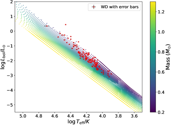
Figure 8. WD evolutionary sequences from A. Bédard et al. (2020) and the WD companions of our golden sample.
Download figure:
Standard image High-resolution imageAs a result, we found that the remaining 133 WD companions have masses ranging from 0.20 to 0.77 M⊙, with a median, 25th, and 75th percentile of  M⊙, thus revealing a population of very-low-mass WDs. Indeed, 26 sources (20% of the sample) have <0.3M⊙ and are therefore considered extremely low-mass (ELM) WDs.
Some authors have suggested that the ELM WDs are likely part of post-common envelope binaries (PCEBs), according to recent studies that found a substantially larger fraction of low-mass WDs in close binaries than in wide binaries. In fact, the latter show a mass distribution similar to that of single WDs (see A. Rebassa-Mansergas et al. 2011 and references therein). According to that hypothesis, low-mass WDs are expected to have suffered mass transfer episodes during their red giant branch (RGB) phase in which its companion cannibalized the WD progenitor, penalizing the final mass of the WD.
Regarding to the MS companions, we estimated their masses (MMS) by means of a cubic spline interpolation of their Teff through the M. J. Pecaut & E. E. Mamajek (2013) tables.
Using the masses MWD and MMS of four of the WDMS eclipsing binary candidates for which the orbital period is known (see Section 3.2) we obtained their semimajor axes, a, using Kepler’s Third Law: ![$a=\sqrt[3]{\left({M}_{\rm{WD}\,}+{M}_{\,\rm{MS}}\right){P}^{2}}$](https://content.cld.iop.org/journals/0004-637X/988/1/51/revision1/apjaddfd7ieqn35.gif) . Not surprisingly, they were found to be very small, with a ranging from ∼0.01 to ∼0.03 au.
. Not surprisingly, they were found to be very small, with a ranging from ∼0.01 to ∼0.03 au.
These results point again toward the PCEB hypothesis, according to which the WD progenitor and its low-mass companion must have been in a relatively tight orbit for mass transfer to occur. If the secondary cannot hold the extra material, both stars could be enveloped in a CE through Roche lobe overflow (B. Willems & U. Kolb 2004).
Within such an envelope, drag forces are expected to remove a significant fraction of the system’s angular momentum, leading to further orbital contraction. The end result would likely be a very close binary system consisting of a low-mass WD and a faint companion star whose mass is too small to produce any noticeable signatures in the system’s astrometry or photometry, which is in keeping with what we observe.
3.5. Comparison with Previous Works
To gain some insight into how many of our WDMS candidates are indeed new identifications, we compared them with the 100 pc volume-limited sample of Gaia EDR3 WDMS binaries from A. Rebassa-Mansergas et al. (2021; hereafter, RM21), finding three common sources. P. K. Nayak et al. (2024; hereafter, N24) used the Gaia CMD but in combination with UV data from GALEX GR6/7, and identified 93 WDMS, two of which are in our sample, but also in RM21. None of our sources are in the catalog of WDMS binaries in open clusters of S. M. Grondin et al. (2024).
We found that 157 sources are in common with the work of J. Li et al. (2025) where the authors used a supervised ML technique known as the Gaussian Process Classifier trained with synthetic data to identify WDMS binaries using the XP spectra of sources among 10 million stars within 1 kpc.
Furthermore, we compared our results with the work of M. L. Kao et al. (2024), where a UMAP allowed the authors to project the XP spectra of the high-confidence WDs from the N. P. Gentile Fusillo et al. (2021) catalog, in a two-dimensional manifold where similar elements fall close to each other. Subsequently, they used the RUWE and a photometric scatter metric to trace the most likely position of the WDMS binaries in the UMAP. As a result, they found an island of 1096 WDMS candidates.
After finding that 368 of our WDMSs are in their catalog, we plotted them in their UMAP as orange and purple triangles (corresponding to sources of our cool and hot WDMS neuron, respectively), as can be seen in Figure 9. The WDMS island found by M. L. Kao et al. (2024) is inside the red circle, where 42 sources of our cool WDMS neuron fell. Not surprisingly, the sources of the hot WDMS neuron are located on the opposite side of the UMAP.
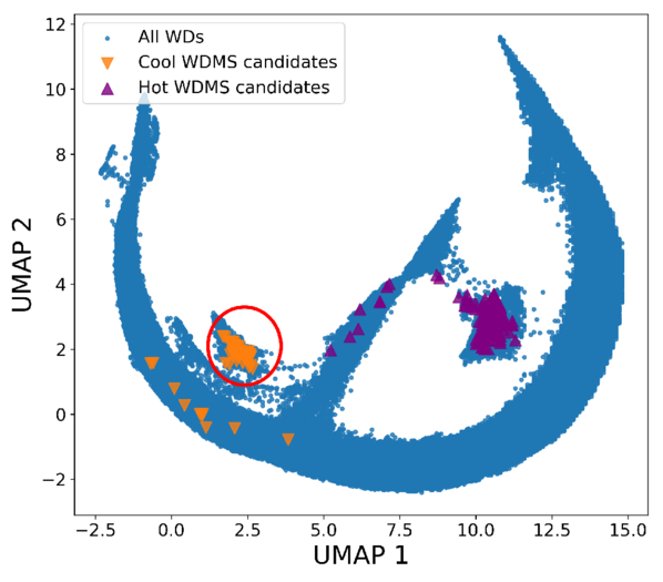
Figure 9. UMAP of M. L. Kao et al. (2024) with WDs in blue and our WDMS binaries in orange. The WDMS island identified by the authors is delineated as a red circle.
Download figure:
Standard image High-resolution imageIt should be noted that our WDMS candidates are located in the regions of the UMAP with higher values of RUWE and photometric scatter (see Figure 5 in their work), demonstrating a strong agreement between the present study and their work.
During the review period of this paper, A. Rebassa-Mansergas et al. (2025) published a new version of their previous work. The authors presented a magnitude-limited catalog of WDMS binaries following a similar methodology as in their previous work (A. Rebassa-Mansergas et al. 2021) to filter the sources. However, this time they were not limited to a specific volume and incorporated synthetic photometry from Gaia XP spectra to improve the quality of their VOSA fits. As a result, A. Rebassa-Mansergas et al. (2025; hereafter, RM25) published a larger catalog of 1312 WDMS, of which 356 are in common with our work. This comparison allows us to report that 506 of our sources are totally new identifications.
Finally, we have compared the WD mass, radius, and Teff of both companions of our golden WDMS candidates with those obtained in RM21, N24, and in A. Rebassa-Mansergas et al. (2025; hereafter, RM25) as shown in Figure 10 and Table 2.
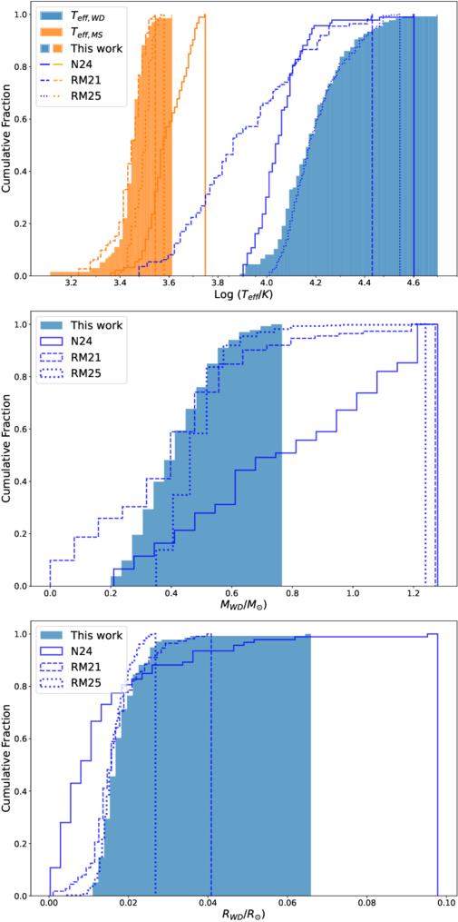
Figure 10. Cumulative Teff distribution for each companion in our golden sample (top), cumulative MWD distribution (middle), cumulative RWD distribution (bottom) and comparison with the corresponding distributions in RM21 and N24.
Download figure:
Standard image High-resolution imageAs can be seen, WDs in our sample are hotter than those in N24 and RM21, although their masses and radii are quite similar, on average, to those in RM21 (though concentrated in a smaller range) thus indicating that our sample belongs to a younger WD population. Moreover, they are lighter and bigger than those found in N24. Furthermore, the cumulative distributions show that our WD primaries are quite similar to those in RM25, with slightly lower masses.
Regarding our MS companions, they are cooler than those in N24 and more similar to those found in RM21 and RM25, except for a small group in the left corner of the distribution, corresponding to the BD candidates found in Section 3.3. This shows that those exotic sources are mostly excluded from previous works.
Table 2. Median, 25th, and 75th Percentile of Some Stellar Parameters Obtained for Our Sample in Comparison with the Works of A. Rebassa-Mansergas et al. (2021), P. K. Nayak et al. (2024), and A. Rebassa-Mansergas et al. (2025)
| Parameter | N24 | RM21 | RM25 | This Work |
|---|---|---|---|---|
| Teff,WD/K |

|

|

|

|
| Teff,MS/K |

|

|

|

|
| MWD/M⊙ |

|

|

|

|
| RWD/R⊙ |

|

|

|

|
Download table as: ASCIITypeset image
Concerning the excess of ELM WDs in our sample, a similar overabundance of low-mass WDs in the Gaia sample has been observed and discussed in A. Rebassa-Mansergas et al. (2021), N. Hallakoun et al. (2024), and J. Li et al. (2025). This coincidence is not surprising, as all of these studies, including this one, focused on unresolved WDMS binaries. Due to Gaia’s high angular resolution and the proximity of these stars (90% of the WDMS in our sample are within 500 pc of the Sun), there is a clear selection bias toward close orbital configurations. Thus, a scenario in which WDs lose mass through stable mass transfer or a CE phase is more plausible.
However, it is also important to note the differences between these works and the present paper. N. Hallakoun et al. (2024) searched for WD companions at ∼1 au of orbital separation from their MS host stars using an astrometric method. J. Li et al. (2025) found most of their binaries in the bridge between the WD and the MS loci, with expected orbital separations of around ∼40 au. The authors therefore argued that stable mass transfer was the most likely mechanism, discarding the CE phase because close orbits are required for it to occur.
In contrast, as explained in Section 2.1, we focused our research strictly on the WD locus, applying astrometric and photometric cuts that biased our sample toward much tighter orbital configurations. Furthermore, as shown in Sections 3.2 and 3.4, we found extremely short orbital periods (P ≈ 0.5 day) and small semimajor axes (a ≈ 0.02 au) in the WDMS candidates with available light curves. These results align more closely with a CE phase that shrunk the orbit (A. Nebot Gómez-Morán et al. 2011; A. Rebassa-Mansergas et al. 2011, 2021). As discussed in Section 3.4, this process could also explain the excess of low-mass WDs.
Nonetheless, we would like to emphasize that firmly establishing the PCEB nature of the objects in our sample requires a much deeper understanding of their orbital configurations, something beyond the scope of this study. We plan to verify these findings through follow-up observations using ground-based telescopes in future work.
During the preparation of this manuscript, A. Santos-García et al. (2025) published a comprehensive statistical study of the unresolved WDMS sample within 100 pc using population synthesis simulations. In their paper, they found that the majority of unresolved WDMS binaries are located in the main sequence (∼90%), and in the intermediate region between the main sequence and the WD region (hereafter, the intermediate WDMS region, ∼10%). In fact, depending on the observational cuts they only expect to find between five and eight WDMS unresolved binaries within 100 pc in the WD region.
To compare our results with their conclusions, we show in Figure 11 our 993 WDMS candidates plotted as blue dots in the Gaia CMD. A subset with the 15 sources that are within 100 pc are highlighted in orange. In black we show the upper boundary of the WD locus as defined in N. P. Gentile Fusillo et al. (2021; hereafter GF21; see Equation 1) used in this work, and in red and blue the upper and lower boundaries of the intermediate WDMS region defined in A. Rebassa-Mansergas et al. (2021) and used in A. Santos-García et al. (2025). As can be seen, only seven WDMS candidates are located below their intermediate WDMS region, which is in excellent agreement with their study.
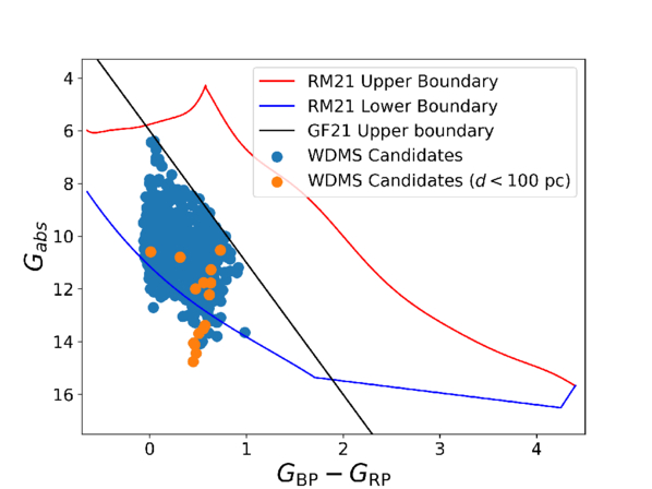
Figure 11. Gaia CMD with the 993 WDMS candidates found in this work, and the boundaries for the WD and WDMS region of N. P. Gentile Fusillo et al. (2021) and A. Santos-García et al. (2025).
Download figure:
Standard image High-resolution imageIn summary, the WDMS candidates found in this work represent a new, different, and complementary population to that previously studied in the literature. However, follow-up observations of our candidates are necessary to confirm their binarity. If verified, our sample of 846 new WDMS binary candidates would increase the total number of known WDMS binary systems by ∼20%.
4. Conclusions
In this work, we have demonstrated the power of self-organizing maps (SOMs) to unveil subtle regularities in the Gaia XP spectra. By combining dimensionality reduction and clustering, our SOM allowed us to identify a thousand of unresolved WDMS candidates in the N. P. Gentile Fusillo et al. (2021) catalog, of which 506 are new identifications.
The analysis presented here illustrates how the SOM can successfully separate WDMS binaries from single WDs based on spectral morphology. Even though our initial sample consists of WD companions that dominate the astrometry and photometry of their systems, our SOM demonstrates an excellent precision (∼90%) in detecting red flux excesses. Unfortunately, the recall is very low because most of the MS companions in the WD locus are being outshined by its degenerated host, as we demonstrated here by comparing their luminosity ratios. Notwithstanding that, our recall is sufficient to recover a third of the WDMS binaries present in the input sample.
We further validated 136 sources in our sample using the VOSA tool to fit binary SEDs with external UV, optical, and NIR photometry together with independent atmospheric models. As a result, we obtained a golden sample for which individual temperatures, luminosities, radii, and masses are estimated.
Using these parameters, we characterized our sample as belonging to a population of atypical low-mass WDs that also include low-mass companions, primarily M dwarfs. A comparison with state-of-the-art WDMS catalogs shows that our method identified a complementary and previously undetected sample of WDMS binaries. This highlights the potential of Gaia DR3 (and the forthcoming DR4) XP spectra combined with unsupervised learning techniques to expand the known WDMS population.
Finally, a cross-match with the Gaia DR3 eclipsing binary catalog shows that at least 13 of our candidates have periodic variability, further supporting their classification as short-period interacting binaries with separations of the order of ∼0.01 au. This subset of systems represents promising targets for follow-up studies.
Acknowledgments
We warmly thank the anonymous referee whose insightful comments have greatly improved this paper. Scientific progress thrives on discussion and collaboration, and this paper is no exception. We are sincerely thank the comments of our colleagues, Alberto Rebassa-Mansergas, Santiago Torres, Raquel Murillo-Ojeda, and Alejandro Santos-García during the 3rd meeting of the Iberian White Dwarf Workshop held in A Coruña in 2025 January. We would also like to acknowledge Nadejda Blagorodnova Mujortova's thoughts on the final version of our manuscript. However, any error is the sole responsibility of the authors. This work has made use of data from the European Space Agency (ESA) Gaia mission and processed by the Gaia Data Processing and Analysis Consortium (DPAC). Funding for the DPAC has been provided by national institutions, in particular, the institutions participating in the Gaia Multilateral Agreement. This work has made use of the Python package GaiaXPy, developed and maintained by members of the Gaia Data Processing and Analysis Consortium (DPAC) and in particular, Coordination Unit 5 (CU5), and the Data Processing Centre located at the Institute of Astronomy, Cambridge, UK (DPCI). This publication makes use of VOSA, developed under the Spanish Virtual Observatory (https://svo.cab.inta-csic.es) project funded by MCIN/AEI/10.13039/501100011033/ through grant PID2020-112949GB-I00. VOSA has been partially updated by using funding from the European Union’s Horizon 2020 Research and Innovation Programme, under grant Agreement  776403 (EXOPLANETS-A). This research was funded by the Horizon Europe [HORIZON-CL4-2023-SPACE-01-71] SPACIOUS project, grant Agreement no. 101135205, the Spanish Ministry of Science MCIN / AEI / 10.13039 / 501100011033, and the European Union FEDER through the coordinated grant PID2021-122842OB-C22. We also acknowledge support from the Xunta de Galicia and the European Union (FEDER Galicia 2021-2027 Program) Ref. ED431B 2024/21, ED431B 2024/02, and CITIC ED431G 2023/01. X.P. acknowledges financial support from the Spanish National Programme for the Promotion of Talent and its Employability grant PRE2022-104959 cofunded by the European Social Fund and E.V. acknowledges funding from Spanish Ministry project PID2021-127289NB-100 is also acknowledged. M.M. acknowledges the funding received from CITIC for a research stay at the IAC. CITIC, as a center accredited for excellence within the Galician University System and a member of the CIGUS Network, receives subsidies from the Department of Education, Science, Universities, and Vocational Training of the Xunta de Galicia. Additionally, it is co-financed by the EU through the FEDER Galicia 2021-27 operational program (Ref. ED431G 2023/01).
Footnotes
- 7
- 8
- 9
- 10
The precision of a class is computed as TP/(TP + FP), with TP being the number of true positives and FP the number of false positives. In simple terms, it provides the probability of the algorithm to be correct when assigning a class to a source.
- 11
The recall is computed as TP/(TP + FN), with FN being the number of false negatives. It indicates the ratio of sources of a given true class that are correctly classified as that class.
- 12