Abstract
The relationship between magnetic activity and Rossby number is one way through which stellar dynamos can be understood. Using measured rotation rates and X-ray to bolometric luminosity ratios of an ensemble of stars, we derive empirical convective turnover times based on recent observations and reevaluate the X-ray activity–Rossby number relationship. In doing so, we find a sharp rise in the convective turnover time for stars in the mass range of 0.35−0.4 M⊙, associated with the onset of a fully convective internal stellar structure. Using MESA stellar evolution models, we infer the location of dynamo action implied by the empirical convective turnover time. The empirical convective turnover time is found to be indicative of dynamo action deep within the convective envelope in stars with masses 0.1–1.2 M⊙, crossing the fully convective boundary. Our results corroborate past works suggesting that partially and fully convective stars follow the same activity–Rossby relation, possibly owing to similar dynamo mechanisms. Our stellar models also give insight into the dynamo mechanism. We find that empirically determined convective turnover times correlate with properties of the deep stellar interior. These findings are in agreement with global dynamo models that see a reservoir of magnetic flux accumulates deep in the convection zone before buoyantly rising to the surface.
Original content from this work may be used under the terms of the Creative Commons Attribution 4.0 licence. Any further distribution of this work must maintain attribution to the author(s) and the title of the work, journal citation and DOI.
1. Introduction
The surge of interest in the nature and conditions of exoplanets and the effects their parent stars have on them has led to a renaissance in the study of the nonthermal emission from stars known very generally as “stellar activity.” This emission originates in the chromosphere and corona and is nonthermal in the sense that it cannot be explained in terms of the blackbody-like thermal spectra that characterize the photospheric emission of stars in general.
The nature of stellar activity was firmly established as a magnetic phenomenon powered by rotation and convection via an interior dynamo in a series of both solar and stellar studies through the 1970s and early 1980s. Observations of Ca II H and K line core chromospheric emission of the Sun revealed a dependence of emission flux on surface magnetic field strength (e.g., E. N. Frazier 1972). In stars, H and K fluxes were found to decrease linearly with the projected rotation velocity (R. P. Kraft 1967), and with stellar age, t, approximately according to t−1/2 (A. Skumanich 1972) due to gradual angular momentum loss through magnetized stellar winds (R. P. Kraft 1967; E. J. Weber & L. Davis 1967; B. Durney 1972; L. Mestel & H. C. Spruit 1987). Higher up in the atmosphere, stellar surveys with the Einstein observatory found that the X-ray luminosity of coronal emission was also highly correlated with the stellar rotation period (R. Pallavicini et al. 1981; G. S. Vaiana et al. 1981; F. M. Walter & S. Bowyer 1981).
The connection of chromospheric and coronal emission with an interior magnetic dynamo indicates that some fraction of the magnetic energy generated finds its way to the stellar surface, and is dissipated by the observed radiative losses and a presumed stellar wind. At present, none of the processes involved in this chain, from the dynamo itself to chromospheric and coronal heating, are fully understood. The dynamo problem alone encompasses the complicated fluid dynamics of rotating, convective, magnetized plasmas at high Reynolds number and over a vast dynamic range of spatial scales that will depend on stellar mass, chemical composition, and rotation rate.
Despite the great complexity of the underlying physics, R. W. Noyes et al. (1984; see also R. W. Noyes 1983) discovered that a remarkably simple pattern emerges from the most elementary consideration of stellar dynamos. R. W. Noyes et al. (1984) noticed that the Ca II flux versus rotation period relation for late-type stars exhibits a systematic scatter whose origin depends on stellar spectral type. This scatter could be greatly reduced if, instead of the rotation period, the ratio of the convective turnover time to the rotation period, Prot/τc, is used. In fluid dynamics, this ratio is essentially the Rossby number, Ro, that describes the ratio of inertial to Coriolis forces. With some simple approximations, the Rossby number can be shown to be related to the dynamo number—the ratio of magnetic field generation to diffusion in the convection zone—as roughly ND ∝ Ro−2 (e.g., B. R. Durney & J. Latour 1978; A. Mangeney & F. Praderie 1984; R. W. Noyes et al. 1984; A. K. Dobson & R. R. Radick 1989; B. Montesinos et al. 2001; N. J. Wright et al. 2011).
While it has been argued that the Rossby number might not be the fundamental underlying scaling for magnetic activity (e.g., G. Basri 1986; R. G. M. Rutten 1987; K. Stepien 1994; A. Reiners & S. Mohanty 2012; A. Reiners et al. 2014), following the work of R. W. Noyes et al. (1984), many other studies have confirmed and extended the Rossby number-based rotation–activity relation using optical and ultraviolet diagnostics of chromospheric and transition region emission (e.g., G. Basri et al. 1985; T. Simon et al. 1985; R. G. M. Rutten 1987; T. Simon & F. C. Fekel 1987; K. Stepien 1994; D. Cardini & A. Cassatella 2007; D. J. Christian et al. 2011; A. Rebassa-Mansergas et al. 2013; E. R. Houdebine et al. 2017; E. R. Newton et al. 2017; M. Mittag et al. 2018; J. S. Pineda et al. 2021; E. M. Boudreaux et al. 2022; X. Li et al. 2024), and based on X-ray diagnostics of coronal emission (e.g., A. Mangeney & F. Praderie 1984; G. Micela et al. 1985; J. H. M. M. Schmitt et al. 1985; A. Maggio et al. 1987; A. K. Dobson & R. R. Radick 1989; C. Jordan & B. Montesinos 1991; N. Pizzolato et al. 2003; N. J. Wright et al. 2011; B. Stelzer et al. 2016; E. González-Álvarez et al. 2019; D. Pizzocaro et al. 2019; E. Magaudda et al. 2022; A. Núñez et al. 2022; Y. Shan et al. 2024; K. G. Stassun & M. Kounkel 2024), including for fully convective M dwarfs (N. J. Wright & J. J. Drake 2016; N. J. Wright et al. 2018; D. Pizzocaro et al. 2019; E. Magaudda et al. 2020).
Of the ingredients in a Rossby number-based description of stellar activity–rotation period and convective turnover time—only the rotation period is directly observable. The convective turnover time, τc, is a measure of the timescale of buoyant convective transport and comes from models of stellar interiors. The original work of R. W. Noyes et al. (1984) employed the convection zone calculations by P. A. Gilman (1980), where τc was evaluated near the bottom of the convective envelope (CE).
Since the seminal work of R. W. Noyes et al. (1984), several studies have reexamined the convective turnover time, both empirically, by demanding that spectral type dependent scatter in rotation versus activity be minimized (e.g., K. Stepien 1994; N. Pizzolato et al. 2003; N. J. Wright et al. 2011), and through numerical stellar evolution models (e.g., R. L. Gilliland 1985; S. M. Rucinski & D. A. Vandenberg 1986, 1990; Y.-C. Kim & P. Demarque 1996; N. Pizzolato et al. 2001; S. A. Barnes & Y.-C. Kim 2010; N. R. Landin et al. 2010; F. Spada et al. 2013; N. R. Landin & L. T. S. Mendes 2017). More recently, E. Corsaro et al. (2021) used asteroseismology to calculate convective turnover times for stars in the mass range 0.9–1.5 M⊙ and calibrate a relation as a function of (B − V) and (GBP − GRP) colors. Of these later studies, only S. A. Barnes & Y.-C. Kim (2010), F. Spada et al. (2013), and N. R. Landin & L. T. S. Mendes (2017) probed the lowest-mass, fully convective M dwarfs. These stars are of special interest in the study of magnetic activity–rotation relations because of recent doubts that have been cast on the general belief of the dynamo in Sun-like stars originating at the tachocline (e.g., N. J. Wright & J. J. Drake 2016; N. J. Wright et al. 2018).
In this work, we recalibrate the relation between convective turnover time and mass for low-mass stars using observations of stellar X-ray emission as a function of the rotation period, and we use the Modules for Experiments in Stellar Astrophysics (MESA r11701) stellar evolution code (B. Paxton et al. 2019) to interpret our results in the context of elementary stellar dynamos. In Section 2, we describe the methods we used to estimate convective turnover times empirically and theoretically. In Section 3, we show the results of both methods and compare them. In Section 4, we interpret our results for empirical and theoretical convective turnover time, discussing implications for magnetic field generation and the stellar dynamo, as well as caveats. Finally, in Section 5, we discuss our conclusions.
2. Methodology
Our data and the methodology through which the convective turnover time is derived are described in this section. Our data are drawn from several sources of measured X-ray luminosities and rotation periods. The convective turnover times (and thereby Rossby numbers) are derived both theoretically, i.e., from stellar models, and empirically. The empirical determination follows that of K. Stepien (1994) and N. J. Wright et al. (2011, 2018). The theoretical understanding of the convective turnover time, herein, follows the 1D stellar evolution and mixing length theory (MLT) presented in L. Henyey et al. (1965) and J. P. Cox & R. T. Giuli (1968).
2.1. Empirical Calculation of Convective Turnover Times
2.1.1. Observational Data
We compiled a catalog of measured ratios of X-ray to bolometric luminosity as well as rotation periods from the literature (see Table 1 for a summary). These data are available alongside our MESA models on Zenodo.11
The majority of this sample comprises solar-type stars with masses larger than the fully convective boundary of ∼0.35 M⊙ retrieved from the work of N. J. Wright et al. (2011). In that study, the X-ray luminosities were computed using the ROSAT bandpass ranging from 0.1 to 2.4 keV, which we also adopt as the reference X-ray luminosity bandpass for the study in hand. When necessary, we converted X-ray luminosities of data from other studies to the same energy band using the webPIMMS tool,12
assuming a plasma/APEC model with  K and NH = 1020 cm−2 for the conversion. If unavailable, we assumed a 20% uncertainty for LX/Lbol, consistent with the mean uncertainties reported in other studies (e.g., B. Stelzer et al. 2016; E. González-Álvarez et al. 2019; E. Magaudda et al. 2020, 2022).
Table 1. Summary of Literature Compilation with X-Ray and Rotation Period Measurements, before and after Quality Cuts
| Catalog | Stars Kept | Total | References |
|---|---|---|---|
| 1451 | 9344 | ||
| SK24 | 629 | 7545 | K. G. Stassun & M. Kounkel (2024) |
| W11 | 386 | 824 | N. J. Wright et al. (2011) |
| N22 | 272 | 440 | A. Núñez et al. (2022) |
| S24 | 56 | 113 | Y. Shan et al. (2024) |
| P19 | 28 | 74 | D. Pizzocaro et al. (2019) |
| M20 | 27 | 54 | E. Magaudda et al. (2020) |
| M22 | 21 | 223 | E. Magaudda et al. (2022) |
| G12 | 21 | 41 | P. Gondoin (2012) |
| W18 | 5 | 16 | N. J. Wright et al. (2018) |
| G13 | 4 | 10 | P. Gondoin (2013) |
| WD16 | 2 | 4 | N. J. Wright & J. J. Drake (2016) |
Download table as: ASCIITypeset image
This base sample was extended by new and archival data provided by E. Magaudda et al. (2020), who homogenized various different catalogs from the literature (B. Stelzer et al. 2016; N. J. Wright & J. J. Drake 2016; N. J. Wright et al. 2018; E. González-Álvarez et al. 2019) to provide a uniform sample of X-ray activity and rotation properties of M dwarfs. We additionally included data for field stars from Y. Shan et al. (2024, CARMENES/ROSAT), K. G. Stassun & M. Kounkel (2024, TESS/eROSITA), E. Magaudda et al. (2022, TESS/eROSITA), and D. Pizzocaro et al. (2019, Kepler/XMM-Newton), as well as data for the open clusters M34, M35, Praesepe, and Hyades from P. Gondoin (2012), P. Gondoin (2013), and A. Núñez et al. (2022, ROSAT/Chandra/Swift observatory/XMM-Newton/K2), respectively.
This resulted in a total of 9344 sources in the base catalog, out of which, only 1451 sources remained in our “clean catalog” after applying various quality cuts to these data. Below, we describe each of the quality cuts, improvements, and considerations we included for our sample.
Crossmatch with Gaia DR3. We performed a simple crossmatch using a 3″ search radius in the Tool for Operations on Catalogues and Tables (Topcat; M. B. Taylor 2005). We found that 98% (i.e., all but 189 stars) of our sample had a match. This allowed us to update the distances in our sample using the most accurate and precise measurements available, and apply the improvements and quality cuts described below.
Remove duplicates. Using the respective Gaia ID, we identified in total 190 stars that had more than one X-ray measurement in our sample. From these, we only removed 10 duplicated sources that had identical measurements of X-ray luminosity, meaning that the same measurement was being included more than once. The duplicated stars with varying values of X-ray luminosity (due to either intrinsic variability of X-ray emission or uncertainty) were kept to improve the calibration of the scatter within the rotation–activity relation.
Remove possible binaries. We subsequently removed stars with renormalized unit weight error (RUWE) > 1.4, which is a parameter provided by the Gaia survey, and allows to filter out stars for which the single-star model does not provide a good fit to the astrometric observations.13 Although extremely useful, the RUWE parameter does not identify tight unresolved binaries. To improve this, we added the cut ipd_frac_multi_peak > 1, which removes stars that are visually resolved double stars. In addition, we used the flag rv_amplitude_robust, which indicates the difference between the largest and the smallest radial velocity measured by Gaia. This number depends on color and magnitude, becoming larger for fainter stars. Therefore, we classified stars as binaries when rv_amplitude_robust > 9 and G < 11. In total, our binary flag removed 2216 stars.
Remove young stars. As we will discuss in more detail in Section 4.2, the convective turnover time depends among other properties on the stellar age. We therefore removed stars younger than 300 Myr for masses <0.6 M⊙, younger than 200 Myr for masses in the range 0.6−0.8 M⊙, and younger than 100 Myr for masses ≥0.9 M⊙. This cut allows us to keep only stars for which the convective turnover time has stabilized, which does not always agree with the convergence into the main sequence. K. G. Stassun & M. Kounkel (2024) included the ages of the stars in their catalog, which we used to apply the cut described above, and for the rest of the sample, we used the Bayesian Analysis for Nearby Young AssociatioNs Σ tool (BANYAN Σ; J. Gagné & J. K. Faherty 2018) to estimate the probability that each star belongs to a known moving group from its position, proper motion, parallax, and radial velocity from Gaia DR3. We removed all the stars that had a probability larger than 0.9 of belonging to a group that would put them in the “young” category according to the cut described above. The cut in age removed 6739 stars, out of which 120 stars were removed using BANYAN Σ. We note that we removed most of the stars in the catalog with this age cut. In addition, we used the position in the color–magnitude diagram (CMD) to identify and remove 106 stars that belonged to the giant branch by visual inspection.
Quality cuts. We applied quality cuts to keep stars with a parallax over error > 20 (equivalent to 5% uncertainty) and also an uncertainty of  smaller than 0.3 dex.
Metallicity. Although we do not have metallicity measurements for our sample, we can take into account several factors that justify the sample being mostly made of stars with solar-like metallicity. R. Kiman et al. (2019) showed that low-metallicity M dwarfs have a locus below the main sequence in the Gaia CMD. When compared to the CMD of our sample, none of the M dwarfs in our sample seem to be low metallicity. In addition, we crossmatched our clean sample with the APOGEE survey (S. R. Majewski et al. 2017; V. V. Smith et al. 2021) and found 245 stars in common (27%). We found that the values for [M/H] are close to solar (between −0.3 and 0.3 dex), which supports the conclusion we obtained from the CMD position of the stars.
Improve mass estimation. We found that the calculations of stellar masses were inconsistent among the different catalogs. In particular, there are known problems with the mass estimation from N. J. Wright et al. (2011; see W.-C. Jao et al. 2022). Therefore, we decided to reestimate the stellar masses for the complete sample by interpolating within the relations provided by M. J. Pecaut & E. E. Mamajek (2013)14 to estimate masses from the absolute G magnitude (MG). This is a precise mass–luminosity relation that is valid for the widest mass range, in contrast to other calibrations that do not cover a wide range of masses (e.g., A. W. Mann et al. 2019; M. R. Giovinazzi & C. H. Blake 2022).
Our final clean sample comprises 1451 stars. We show a summary of the compiled sample in Table 1 and the X-ray luminosities as a function of the rotation period for the clean sample of stars color-coded by mass in the left panel of Figure 1.
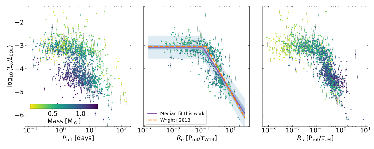
Figure 1. The ratio of the X-ray to bolometric luminosities of our clean sample of stars (see Section 2.1.1 for a description of the sample) as a function of stellar rotation period (left panel), Rossby number calculated using the convective turnover times determined by N. J. Wright et al. (2018) for masses between 0.4 and 0.9 M⊙ (middle panel), and the theoretical convective turnover time τcM at 1 Gyr from in this work (see Section 2.2 for the definition; right panel). The color of each point denotes the stellar mass, as indicated in the color bar. We show our fit to the data in the middle panel: the purple line denotes the fit median using Equation (1); 2000 random samples from the posterior of the parameters are shown in blue shade, and the fit to the scatter of the relation is shown in light-blue shade. The orange dashed line shows the fit obtained by N. J. Wright et al. (2018).
Download figure:
Standard image High-resolution image2.1.2. Empirical Approach
The Rossby number description of stellar activity requires the stellar rotation period in combination with the convective turnover time. The turnover time can be calculated empirically by finding the parameter that reduces the scatter in the activity–rotation relation (e.g., R. W. Noyes et al. 1984; K. Stepien 1994; N. J. Wright et al. 2011, 2018). In this section, we describe our calculation of the empirical calculation of the turnover time, τcE, following the methods outlined in N. J. Wright et al. (2011, 2018). This method allows us to determine τcE as a function of mass under the assumption that all stars follow the same two-step piecewise relationship of LX/Lbol as a function of their Rossby number, Ro (defined as Ro = Prot/τcE, where Prot is the stellar rotation period),

where C is a normalization constant, and Rosat is the Rossby number at which the transition from saturated to unsaturated regimes occurs. The implication of Equation (1) is that all masses share the same saturated value of  , and all masses become unsaturated at the same value of Rosat and, for higher values of Ro, follow the same power-law dependence of LX/Lbol with Ro.
In order to determine the values of  , Rosat, and β for our stellar sample, we fit Equation (1) to the observations, where
  . To compute Ro, we first used the convective turnover times provided by N. J. Wright et al. (2018). As we discuss in Section 3.2, the functional form of the empirical calibration from N. J. Wright et al. (2018) differs significantly from the models for high (>1 M⊙) and low (<0.4 M⊙) masses. Therefore, to avoid biasing our fit, we perform this first fit only to masses in the range 0.4−0.9 M⊙. The rest of the analysis will be done using the complete sample. The ratios of LX/Lbol as a function of Ro for the selected mass range of the sample are shown in the middle panel of Figure 1. As we cannot see evidence of supersaturation in our sample, we did not include this phenomenon in the fit; however, we cannot discard that there might be a significant effect for the fastest rotators (Prot < 1 day, e.g., S. Randich 1998; D. J. James et al. 2000; C. Argiroffi et al. 2016).
We used the Markov Chain Monte Carlo sampler implemented in emcee (D. Foreman-Mackey et al. 2013) to determine β,  , and Rosat. In addition, we included a parameter σ to fit the scatter of the relation and obtain a more precise estimation of uncertainties. We defined the likelihood of the model as
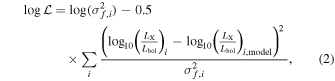
where  is calculated using Equation (1), and
  is the sum of the uncertainty of the X-ray fractional luminosity squared and the characterization of the scatter of the relation squared (
 ). To obtain the posterior, we combined the likelihood described above with flat priors for each of the parameters such that 0.01 < Rosat < 1, −5 < β < −1,
  , and 0 < σ < 5.
We report the median of the posterior as the parameter estimate, and the symmetric interval surrounding the median that contains 68.3% of the posterior distribution as the uncertainty. We find β = −1.96 ± 0.08, Rosat = 0.11 ± 0.01, and  , and σ = 0.40 ± 0.01. The parametric fit to the data is also shown in the middle panel of Figure 1, where we show the median together with 2000 random samples from the posteriors of each parameter and the fit to the scatter of the relation. We note that our fit agrees within uncertainties with the results from N. J. Wright et al. (2018) shown in an orange dashed line in Figure 1 (
 ,
,  , and
, and  ).
).
With β and  determined, we now fix the parameters β = −1.96 and
  . In addition, we fixed σ = 0.40. These assumptions allow us to determine the rotation period at which saturation occurs for groups of stars of approximately equal mass, independently of the convective turnover time. We divide our sample into 14 mass bins ranging from 0.1 to 1.2 M⊙, with approximately equal numbers of stars in each bin, and fit the equation

using the grid sampling method to obtain the probability distribution of Psat per mass bin. emcee is significantly slower when we only fit for one parameter, so we decided not to use it in this case. The mass-dependent constant  can also be defined as
  using Equation (1), which now allows for the determination of τcE as a function of stellar mass. We show the individual fits to each mass bin in Figure 2. By visually inspecting each of the fits, we find that most of them agree with the data. There is a small difference between fit and data for the two highest-mass bins: 1.01 M⊙ and 1.09 M⊙. In these two cases, the slope seems to be less steep in the data. It is possible that the relationship between activity and rotation rate would change toward higher masses, as more massive stars have vanishingly thin CEs (disappearing perhaps after 1.3 M⊙). So, it might be expected that the relation should change toward higher masses at some point, as the magnetic dynamo correspondingly becomes ineffective. However, we cannot confirm this difference because we do not have enough saturated stars to fully characterize the relation. We note that the difference between data and fit is not large enough to affect the discussions in the rest of the paper.
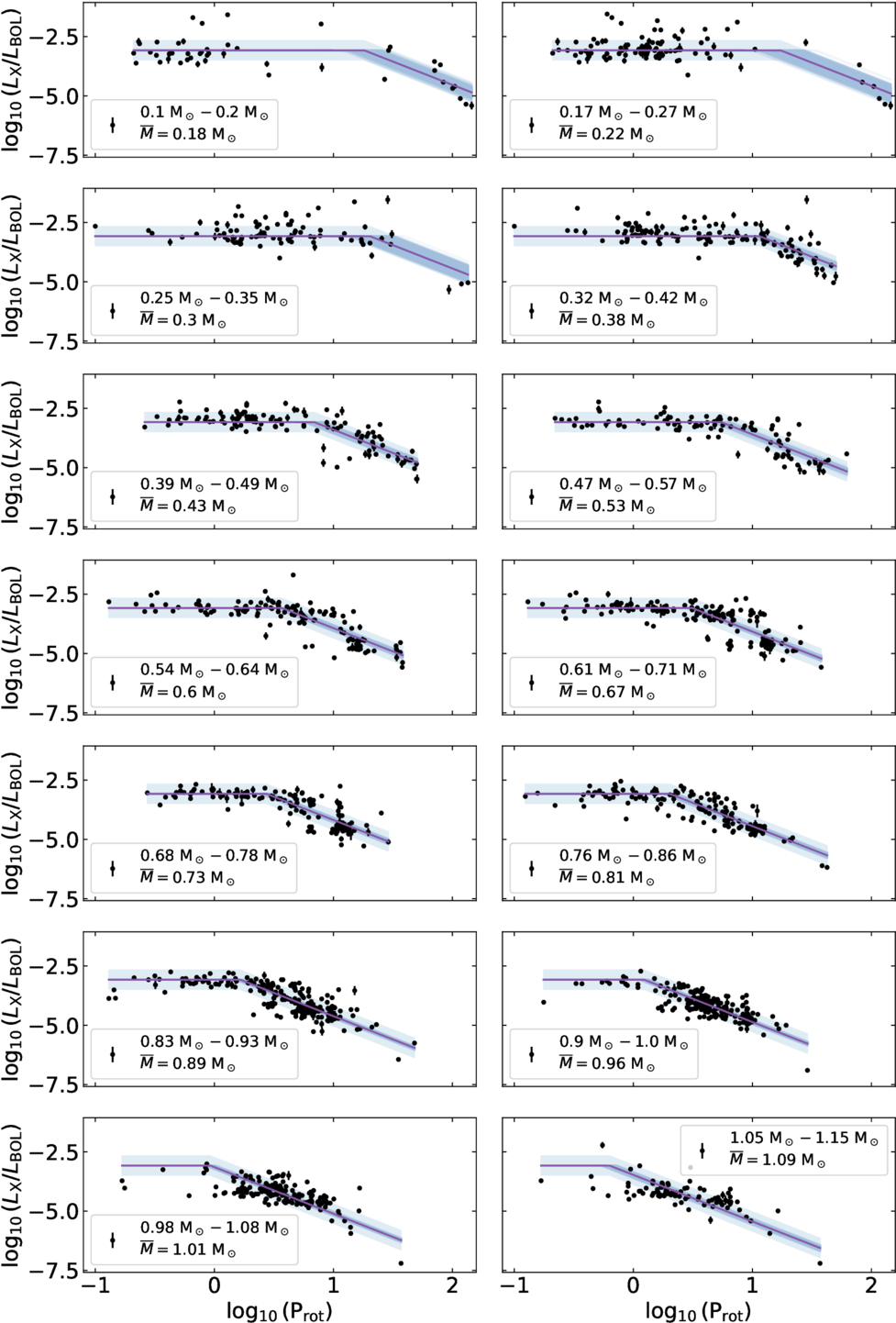
Figure 2. The X-ray luminosity as a function of rotation period (black points) for the different mass bins. The purple solid lines illustrate the best-fit piecewise function (Equation (3)) to locate the rotation period at which stars transition from the saturated regime to the unsaturated regime of X-ray activity. Each panel is labeled with the mass range of the stars included in the fit. We included 2000 random samples of the posterior for Psat and a light-blue band that shows the scatter of the relation.
Download figure:
Standard image High-resolution imageWe confirmed previous results that the rotation period at which saturation occurs clearly increases with decreasing stellar mass (e.g., N. Pizzolato et al. 2003; E. R. Newton et al. 2016; N. J. Wright et al. 2018; and references therein). As mentioned above,  , which means that we calculate the convective turnover times using
  . This leaves a constant C to be determined, which will affect the normalization of our calculations of τcE, but not the relative values, as noted also in previous studies (N. Pizzolato et al. 2003; N. J. Wright et al. 2011). N. J. Wright et al. (2011, 2018) decided to choose this normalization, so that their solar value for τc agrees with the value in R. W. Noyes (1984), which was theoretically derived. Unfortunately, there is no precise independent estimation of the solar convective turnover time that could be used to normalize our values (W.-C. Jao et al. 2022); therefore, we need to choose between other calibrations. As we are interested in comparing our empirical values with our model values of convective turnover times (τcM, described in Section 2.2), and with the empirical values obtained by N. J. Wright et al. (2018), we defined C such that τcE agrees with our theoretical calculations for the mass bin corresponding to 0.96 M⊙. This particular mass bin is the closest to the solar-mass bin that has the highest number of stars, which makes the fit to the X-ray versus rotation period more precise (see Figure 2). Furthermore, the values for τc from N. J. Wright et al. (2018) and our theoretical calculations (14.8 and 14.6 days, respectively) agree in this bin, which allows the comparison of our empirical τcE with both calibrations. To calculate the uncertainties of τcE, we did a Monte Carlo propagation of uncertainties of all parameters involved in the calculation (Psat, β, and
  ). We note that, although β and
  were fixed to calculate Psat, the uncertainty of the first fit was included in the calculation of Psat given that we included the parameter σ to characterize the scatter of the relation. The masses and uncertainties for each bin were calculated as the median mass of the bin and the standard deviation, respectively. The resulting convective turnover times calculated with the empirical method are shown in Figure 3.
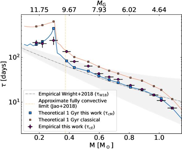
Figure 3. Empirically derived value of τcE from this work (dark purple points, for each mass bin), compared to the empirically derived τW18 using the relation of N. J. Wright et al. (2018; gray dashed line and uncertainty in light gray), and the calculated τcM from the MESA models for 1 Gyr via the new approach described in Section 2.2.2 (blue squares) all as a function of stellar mass. In addition, we included the convective turnover times calculated with the classical formalism of, e.g., R. L. Gilliland (1985; orange squares).
Download figure:
Standard image High-resolution image2.2. Theoretical Calculation of Convective Turnover Times
In order to interpret the empirical τcE values, we calculated theoretical convective turnover times, τcM, using stellar evolutionary models. In making this comparison, we are tacitly accepting the paradigm wherein the empirical turnover time is in fact the same as the theoretical turnover time. In doing so, our aim is to present a physical interpretation of the empirical turnover time by examining correlated stellar properties.
2.2.1. Stellar Structure Model Calculations
In order to examine stellar structure model calculations of the convective turnover time, τcM, we used MESA, simulating stars in the mass range 0.1–1.3 M⊙ with solar metallicity and a ratio of mixing length to pressure scale height αMLT = 1.82. Our model profiles as well as full history output at 1, 5, and 14 Gyr, plus inlist and source files, are available on Zenodo.15 Many of our underlying physical assumptions are derived from the MISTv1.2 models (J. Choi et al. 2016), based on calibrations described in that text. The value of αMLT = 1.82 can affect the convection zone size of stellar models, with larger values leading to deeper convection zones. While our choice of αMLT follows from a calibration to solar helioseismic data (J. Choi et al. 2016), it is similar to the value of 2 chosen by R. W. Noyes (1984). There, it was found to minimize the scatter of the activity–rotation relationship and was also noted to reproduce solar values.
We summarize a number of the most salient parameter adoptions made for our models in Table 2 and refer to it for values of the parameters described below. As stated above, most of these values are unchanged and adopted from MIST (J. Choi et al. 2016), to which we refer the reader for further details. In our models, as we are using MESA version r11701; the standard amalgamation of equation of state tables is now augmented by the PTEH tables covering especially low density material (see B. Paxton et al. 2019). Similarly, we use a standard amalgamation of opacity tables.
Table 2. A Selection of Adopted Parameters in Our MESA Models
| Ingredient | Adopted Parameters | References |
|---|---|---|
| Solar abundance scale | X⊙ = 0.7154Y⊙ = 0.2703, Z⊙ = 0.0142 | (a) |
| Equation of state | OPAL+SCVH+MacDonald+HELM+PC+PTEH | (b, c, d, e, f, g) |
| Boundary conditions | M ≤ 0.5 M⊙: tau_100_tables, off table: gray and_kap | (h) |
| M > 0.5 M⊙: simple_photosphere | ||
| Opacities | OPAL Type I for T ≳ 104 K; Ferguson for T ≲ 104 K | (i, j) |
| OPAL Type I → Type II post-TAMS | ||
| Convection | αMLT = 1.82 (solar calibrated), ν = 1/3, y = 8 | (k) |
| Overshoot | time-dependent, diffusive, 
| (l) |
| Semiconvective mixing | αsc = 0.1 | (m) |
| Thermohaline mixing | αth = 666 | (n, o) |
| Winds (mass loss) | Reimers (ηR = 0.1) for the main sequence and red giant branch | (q) |
| Blöcker (ηB = 0.2) for the asymptotic giant branch | (r) |
Note. Unless otherwise noted in the text, values are adopted from MIST (J. Choi et al. 2016), which may be consulted for further details.
References. (a) M. Asplund et al. (2009), (b) F. J. Rogers & A. Nayfonov (2002), (c) D. Saumon et al. (1995), (d) J. MacDonald & D. J. Mullan (2012), (e) F. X. Timmes & F. D. Swesty (2000), (f) A. Y. Potekhin & G. Chabrier (2010), (g) O. R. Pols et al. (1995), (h) B. Paxton et al. (2011), (i) C. A. Iglesias & F. J. Rogers (1993, 1996), (j) J. W. Ferguson et al. (2005), (k) L. Henyey et al. (1965), (l) F. Herwig (2000), (m) N. Langer et al. (1983), (n) R. K. Ulrich (1972), (o) R. Kippenhahn et al. (1980), (p) A. Heger et al. (2000), (q) D. Reimers (1975), and (r) T. Blöecker (1995).
Download table as: ASCIITypeset image
Our choices for the treatment of convection derive from the calibrated parameterizations utilized in J. Choi et al. (2016). Namely, our convective overshooting follows the time-dependent, diffusive, F. Herwig (2000) exponential overshooting scheme. In this scheme, overshoot mixing is parameterized through a diffusion coefficient scaled by a free parameter fov. This free parameter can take on different values in the core ( ), shell (fov,sh), or envelope (fov,env) of the model.
As we utilize the Ledoux criterion, regions that are convectively unstable according to the Schwarzschild criterion may be stabilized by a positive composition gradient, leading to semiconvective mixing. In the opposite case of a thermally stable region destabilized by a negative composition gradient, thermohaline mixing can arise. Both thermohaline and semiconvective mixing enter as time-dependent diffusive processes, parameterized by diffusion coefficients (as in R. K. Ulrich 1972; N. Langer et al. 1983), scaled by free parameters αth and αsc, respectively.
Mass loss for these models follows the same scheme as used in the MIST models of J. Choi et al. (2016). Most relevant for the mass range under study are the wind schemes used to describe mass loss on the main sequence and red giant branch (RGB; D. Reimers 1975) and on the asymptotic giant branch (AGB; T. Blöecker 1995). The mass-loss rates described by D. Reimers (1975) and T. Blöecker (1995) are scaled by free parameters ranging from 0 to 1 denoted as ηR and ηB in Table 2. The adopted values were tuned by J. Choi et al. (2016; see references therein) to match observational constraints that include the initial–final mass relation, the AGB luminosity function, and asteroseismic constraints from Kepler.
Lastly, compared to J. Choi et al. (2016), we adopt a simplified set of boundary conditions. We utilize the atmosphere tables referred to as simple_photosphere for masses above 0.5 M⊙. This option calculates the temperature using the Eddington T(τ) relation, assuming τ = 2/3, and calculates the pressure similarly utilizing an expression for hydrostatic equilibrium. As noted in J. Choi et al. (2016), the simple_photosphere tables can be a poor choice in some cases.
We calculated models that use MESA’s photosphere_tables, which are fully modeled atmosphere tables as described in B. Paxton et al. (2011) as well in this mass range; ultimately, these alternate models made no difference to our results. For lower masses, we adopt a combination of MESA’s tau_100_tables and grey_and_kap tables for density and temperature values not covered by the former (see B. Paxton et al. 2011 for more on these tables). This choice is motivated similarly to the choice made in J. Choi et al. (2016), where anchoring the boundary condition to a point deeper in the atmosphere (at τ = 100 in this case) can provide a more realistic model for low-mass stars whose outer envelopes are heavily influenced by molecules not accounted for by MESA’s standard atmosphere tables.
These are 1D stellar models evolved to an age of 1 Gyr, by which time stars in this mass range have settled onto the main sequence. On the main sequence, the convective turnover time has mostly stabilized to a single value and only changes slightly with time. Our models are nonrotating, and while rotation can affect the stellar structure, and thus convective boundaries, we find that such effects are relatively small. Our models are of the solar metallicity (Z⊙ = 0.0142 from M. Asplund et al. 2009), and while metallicity variations can substantially alter convection zone size, we find the majority of our observed stars are near solar metallicity (see Section 2.1.1); although, we aim to explore the effect of metallicity variations in greater detail in future work.
Stars less than approximately 1.3–1.4 M⊙ possess CEs that start off extremely thin at the higher-mass end (A. C. Beyer & R. J. White 2024), and eventually extend all the way to the core at around M ≲ 0.35 M⊙, as determined via the “Ledoux criterion” (P. Ledoux 1947) implemented in the MESA models. At 1 Gyr, stars in this mass range are also primarily on the main sequence, when interior conditions and parameters are mostly changing only very slowly (see, e.g., Y.-C. Kim & P. Demarque 1996; N. R. Landin et al. 2010), and are representative of all but the very lowest-mass stars in young open clusters as well as the Galactic disk.
2.2.2. Theoretical Approach
The convective turnover time is a quantity typically understood through MLT (via L. Henyey et al. 1965; see M. Joyce & J. Tayar 2023 for a review) that quantifies the timescale of convective motion. It is a local quantity, calculated at a position r within a stellar model as

where vc(r) is the local convective velocity, and HP(r) is the local pressure scale height. Thus, τc(r) is the local ratio of the pressure scale height to convective velocity at some location r in the CE, taking on well-defined values in convection zones. It is common to scale HP by some factor, αMLT, the mixing length parameter, which typically ranges in value from 1 to 2, depending on the model. We neglect the scaling factor of αMLT, and calculate τc as in Equation (4). To calculate the Rossby number (Ro = Prot/τc), one must then decide on the appropriate position r to use when calculating τc(r).16
For example, as noted in Section 1, R. W. Noyes (1984) used the convective turnover time calculations of P. A. Gilman (1980). The models of P. A. Gilman (1980; similar to calculations made by B. R. Durney & J. Latour 1978) calculated τc with HP(r) evaluated at the bottom of the CE (r = rBCE), and vc(r) at one pressure scale height above rBCE (at r = rBCE + HP(rBCE); see also R. L. Gilliland 1985). In the context of stellar dynamos, these choices were made under the consideration that solar and stellar (αΩ) dynamos are thought to reside near the tachocline (near r = rBCE).
We take Equation (4) as the definition of τc and test the assumption that the dynamo may lie near rBCE in our analysis. In calculating τc, there is some subtlety in calculating HP, motivating a slightly different calculation method from P. A. Gilman (1980) to calculate τc in our work that we describe below. Throughout the text, we use τcM and τcE to refer to our model and empirical τc, respectively.
2.2.3. Evaluating HP(r) above the Convection Zone Base
Here, we outline complications of calculating HP in fully convective models and our handling of them. Classically, HP is calculated as HP(r) = P(r)/g(r)ρ(r); with P(r) being the local pressure, g(r) being the local gravitational acceleration, and ρ(r) being the local density, all functions of the radius r. In fully convective stars, rBCE is simply the center of the star. Here, g(0) → 0, causing HP(0) to diverge under the definition above for fully convective stars. This is problematic for the classical definition of the convective turnover time that evaluates HP(r) at r = rBCE (P. A. Gilman 1980; R. L. Gilliland 1985).
In MESA, the divergence of HP is handled by switching to an alternate definition near the center of the star (P. P. Eggleton 1971), ![${H}_{{\rm{P}}}^{{\prime} }(r)={[P(r)/G{\rho }^{2}(r)]}^{1/2}$](https://content.cld.iop.org/journals/0004-637X/988/1/102/revision1/apjadde4dieqn25.gif) when
when  (as described in B. Paxton et al. 2011, Section 5.1). While this avoids the numerical trap of infinite scale height at the stellar center, it still represents a discontinuity in the treatment of HP(r) below the fully convective limit. In the fully convective regime, this would then be using the P. P. Eggleton (1971) formula for
  and the classical expression for HP(r) in the partially convective regime. Additionally, as vc(r) → 0 at r = rBCE, P. A. Gilman (1980) calculated vc(r) at a different position from HP(r), i.e., at r = rBCE + HP(rBCE), one pressure scale height from the bottom of the CE (R. L. Gilliland 1985).
We choose to evaluate both HP(r) and vc(r)—and thus τc(r)—at the same position, hereafter called  . Conceptually,
  is similar to where R. L. Gilliland (1985; and P. A. Gilman 1980) calculated vc(r) in their models. We utilize

which is the bottom of the CE plus half of a (local) pressure scale height. However, rather than setting r = rBCE in Equation (5) (as in classical works), we solve for the position r to evaluate τc(r) as follows.
Starting from the surface of the 1D stellar model, we advance inward cell by cell. At each ith model cell, we evaluate

and stop iterating when Equation (6) is satisfied, taking r = ri. If we rearrange Equation (6), one may see that we are solving

where Δri ≡ ri − rBCE is an extended distance above the bottom of the convection zone, i.e., the distance from the bottom of the convection zone to the ith cell above it. Equation (7) is satisfied when this distance becomes comparable to half the local pressure scale height in the CE. In our MESA models, this locale lies near the bottom of the CE, but always above where  and therefore presents a consistent treatment of HP, regardless of convection zone depth. We then use r = ri with Equation (4) to estimate our model convective turnover times, τcM.
Going forward, we operate under the framework that the empirical convective turnover time (τcE, described in Section 2.1.2) is comparable to the theoretical turnover time. Accordingly, we consider that the empirical value correlates to τc(r) evaluated at a particular position (r) within the stellar model. The implication is that this position corresponds to the mean location of the magnetic dynamo, as revealed through the activity–Rossby relationship.
3. Results
3.1. Empirical Convective Turnover Times
The empirically derived τcE for each mass bin via the methods of Section 2.1 is shown in Figure 3 and Table 3. We also show a comparison of our empirically derived τcE to the empirically derived τW18 in N. J. Wright et al. (2018), and to the convective turnover times, τcM, provided by the MESA models described in Section 2.2. The G-band absolute magnitude used to estimate masses (Section 2.1.1) is shown on the top axis.
Table 3. Results for Our Theoretical (τcM) and Empirical (τcE) Calculation of Convective Turnover Time
| Mass | τcM | τcE | n |
|---|---|---|---|
| (M⊙) | (days) | (days) | |
| 0.18 ± 0.03 | 194 | 213.12 ± 30.63 | 46 |
| 0.22 ± 0.03 | 225 | 202.31 ± 38.52 | 99 |
| 0.30 ± 0.03 | 441 | 238.12 ± 49.10 | 89 |
| 0.38 ± 0.03 | 83 | 134.38 ± 9.84 | 127 |
| 0.43 ± 0.03 | 59 | 80.90 ± 5.88 | 119 |
| 0.53 ± 0.03 | 49 | 63.75 ± 4.67 | 101 |
| 0.60 ± 0.03 | 39 | 43.30 ± 2.50 | 128 |
| 0.67 ± 0.03 | 32 | 36.50 ± 1.77 | 162 |
| 0.73 ± 0.03 | 27 | 32.24 ± 1.63 | 133 |
| 0.81 ± 0.03 | 22 | 23.77 ± 1.25 | 141 |
| 0.89 ± 0.02 | 19 | 19.36 ± 0.73 | 208 |
| 0.96 ± 0.03 | 14 | 14.48 ± 0.52 | 194 |
| 1.01 ± 0.03 | 12 | 10.88 ± 0.41 | 176 |
| 1.09 ± 0.03 | 7 | 7.41 ± 0.41 | 90 |
Download table as: ASCIITypeset image
The main feature in Figure 3 is the significant increase in convective turnover time around the fully convective boundary (0.35 M⊙) we found with our calculation of τcE, which was not present in the previous empirical calibration τW18 (N. J. Wright et al. 2011, 2018). In addition, we found that for masses >0.9 M⊙ our calculations of τcE are smaller than the τW18, and that this difference increases as the mass increases. We note that, as explained in Section 2.1.2, there is a rather arbitrary normalization involved in the calculation of τcE. In this case, the normalization was chosen so τcE and τcM agree at 0.96 M⊙, which also agrees with τW18, and allows the comparison of our calculations to both calibrations.
We divided the mass range into 14 bins with a 0.1 M⊙ size. This choice resulted in a smooth trend of convective turnover time as a function of mass, and a similar number of stars in each bin. The final results were insensitive to the exact size and number of bins.
As described in Section 2.1.1, we removed binaries from the sample using quality cuts from Gaia. However, these cuts are not 100% efficient at removing binaries. Therefore, we examined if the results in Figure 3 changed if we included the binaries, and if we were more strict with the binary cuts (for example, including a cut according to the position in the CMD). We found that the results stay the same, and the features did not change significantly. To further test our method for systematic errors, we reran only the sample from N. J. Wright et al. (2018) with masses from the literature to estimate the convective turnover time as a function of mass and were able to reproduced their results. Furthermore, we found that, when using the masses estimated using MG with the sample from N. J. Wright et al. (2018), there is a slight trend that shows that the convective turnover time increases at the fully convective boundary, albeit not as clear as in Figure 3 given that our sample contains a significantly larger number of stars. This shows the importance of estimating accurate masses for this analysis.
3.2. Comparison between Empirical and Model τc
We show our MESA turnover times (τcM) in Figure 3 as the blue squares and line. Values of τcM show generally good agreement with τcE for (partially convective) masses 0.4 M⊙ < M⋆ < 1 M⊙, and again for (fully convective) M⋆ < 0.3 M⊙. Qualitatively, the model and empirical values agree fairly well across the entire mass range. Our empirical and model turnover times in particular follow quite closely the relation of N. J. Wright et al. (2018) over all masses in terms of the slope. However, owing to our larger data set and different mass estimates, there is a notable difference at lower masses, particularly in the range 0.3–0.4 M⊙, within which stellar structure is expected to transition from being partially to fully convective (e.g., G. Chabrier & I. Baraffe 1997; W.-C. Jao et al. 2018). This feature appears as a peak in the empirical convective turnover time values that are matched relatively well (in a qualitative sense) by the theoretical values. We note that the point corresponding to a median mass of 0.3 M⊙ has a τc value smaller than the model (blue square), which is consistent with averaging several points over the sharp feature.
We show the activity (LX/Lbol)–Rossby relation using our theoretical convective turnover time, τcM, in the right panel of Figure 1. As expected, the scatter in the relation is significantly reduced compared to LX/Lbol as a function of the rotation period (left panel) and of Rossby number of N. J. Wright et al. (2018; middle panel).
We included in Figure 3 the theoretical calculation of convective turnover times using the classical formalism, described in Section 2.2, shown by the orange dots and line for comparison. These values are slightly higher than our empirical calculations. However, as noted in Section 2.1.2, there is a normalization that was chosen so the empirical values agree with the calibration of our theoretical values τcM and from N. J. Wright et al. (2018). When normalizing to the classical τ values, we found good agreement between our τcE and the classical τ, except for the two least massive bins. Our empirical τcE agrees better with our theoretical τcM than the classical τ. However, as can be seen in Figure 2, these two low-mass bins do not have enough stars to clearly distinguish between the two models. More data are needed for the lowest stellar masses to identify the correct formalism. We note that the differences between our τcM and classical τ are small enough that it does not impact the conclusions and discussions in our analysis, with both following a similar trend versus stellar mass.
Our models provide some insight into the nature of the spike in τcM. The CE sizes from our MESA models at 1 Gyr are illustrated in Figure 4. Our models suggest that the base of the solar convection zone lies at roughly 0.7 R⋆ at this age, which decreases to about 0.6 R⋆ at 0.4 M⊙. At 0.4 M⊙, an important transition occurs in which there is a precipitate deepening between 0.4 and 0.35 M⊙ where the convection zone as a function of mass rapidly plunges toward the stellar center. At lower masses still (M ≲ 0.35 M⊙), our models are fully convective.
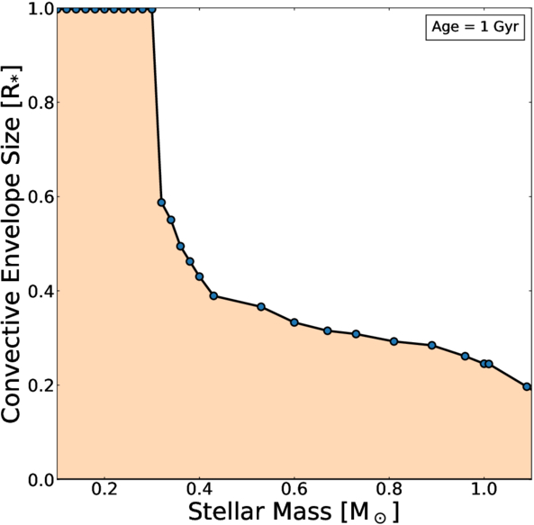
Figure 4. The CE size according to the Ledoux criterion, expressed as a fraction of total stellar radius in late-type stars of solar chemical composition at 1 Gyr as a function of stellar mass.
Download figure:
Standard image High-resolution imageAs explained in G. Chabrier & I. Baraffe (1997), the onset of the fully convective limit involves a competition of factors that promote the growth of a convective core and a deepening of the convection zone. When the convective core and outer CE meet, the star may be considered fully convective, leading to the sudden jump in the CE size. This rapid deepening of the CE toward lower masses coincides with the rapid rise in τcM and τcE.
3.3. The 0.3 M⊙ Peak in τc as Seen in Theory
To understand why our calculations of τcM rise with CE depth, we illustrate the variation with the depth of τc(r) together with other convection zone properties for different stellar masses in Figure 5 (blue line); we also note the location where τc(r) = τcE (the purple dot). This figure will be discussed in further detail in Section 4.1 below. We note here that, for all masses, τc(r) is an increasing monotonic function of the depth within the convection zone.
In the context of Equation (4), τc(r) rises with depth due to an increase of HP(r) with depth and a decrease of vc(r) toward the bottom of the convection zone. In essence, convective motion slows with depth in part due to the weight of overlying material and the effective gravity being diminished toward the stellar center, but also due to the weakening of superadiabaticity, ∇ − ∇ad with depth, which (under MLT, J. P. Cox & R. T. Giuli 1968) vc is a function of. Here, ∇ represents the actual temperature gradient, and ∇ad is the adiabatic temperature gradient, with a superadiabatic temperature gradient being a prerequisite for convective transport to occur. By design, our calculations of τcM lie near the bottom of the convection zone (Section 2.2.2, blue dot in Figure 5), and so increase as the convection zone deepens toward the fully convective limit, and as the CE grows in mass.
As for why τcM then decreases again for masses ≲0.3 M⊙, we note that, once a star becomes fully convective, the bottom of the convection zone becomes fixed (i.e., it is the center of the star). In Figure 5 (bottom row), we see that the location corresponding to τcE begins to settle around r = 0.2 R⋆. Thus, from our modeling, we can say that, as this position becomes fixed, and as the stellar radius decreases with stellar mass, the effective CE above this position becomes shallower. As argued above, this causes a decrease in the value of the convective turnover time at this location, leading to the fall in values of τcM (and presumably τcE) toward lower masses, after the peak, that we see in Figure 3. To help demonstrate these points, we show the variation of τc, HP, and vc in the right-hand panel of Figure 6 for several masses. The mass exterior to  versus stellar mass (i.e., the effective CE above this position) is shown in the left panel. The interplay of thermodynamic properties does not yield a simple scaling with stellar mass, but in general as the size of the effective CE decreases with mass below 0.3 M⊙, the HP at r = 0.2 R⋆ shrinks as well (while changes in vc at this point are comparably slight), thus yielding generally smaller τcM with decreasing mass. A similar effect occurs at higher masses, approaching 1.3 M⊙ as the CE begins to more rapidly shrink in size (as may be seen from Figure 4).
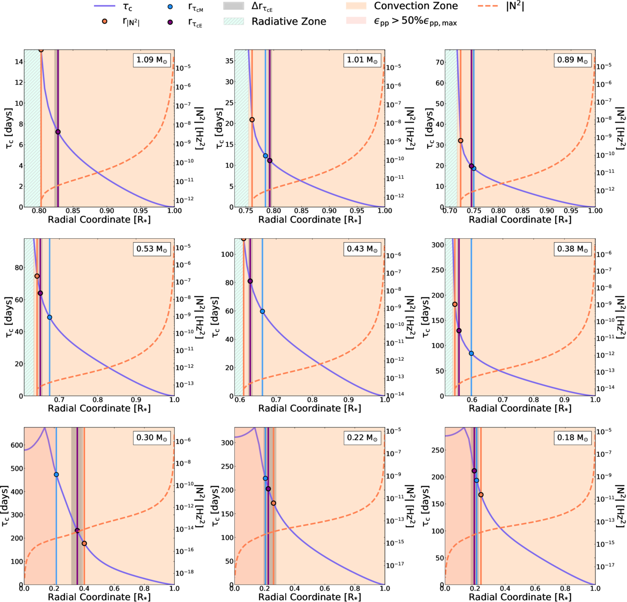
Figure 5. Stellar profiles at an age of 1 Gyr, each panel corresponding to a stellar mass indicated in the upper right, that show the variation of the convective turnover time on the left-hand y-axis (solid blue line) and absolute value of the Brunt–Väisälä frequency (dashed dark orange line) on the right-hand y-axis. The stellar surface lies at the right-hand side of the plot, and the interior lies toward the left. Points along the solid blue curve showing τc(r) indicate where values of τcM (blue dot), τcE (purple dot), and  (dark orange dot) exist in the stellar model. Corresponding vertical lines are to show the inferred position in the stellar model. The gray band around the vertical line of τcE indicates the uncertainty on the inferred location of τcE. Orange regions represent convection zones, and hatched turquoise represents radiative zones. Pink shaded regions indicate where the nuclear energy production rate (via the p–p chain,
 pp) is greater than 50% of its peak value. The inflection points in the 0.18−0.3 M⊙ model τc(r) correspond to where the pressure scale height definition changes to the P. P. Eggleton (1971) prescription (see Section 2.2.2).
Download figure:
Standard image High-resolution image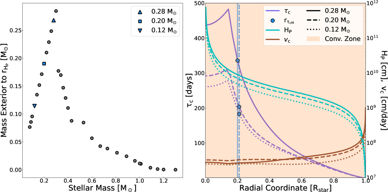
Figure 6. Left: the mass exterior to the position  , showing that at the high-mass end relatively little mass lies on top of the CE; this increases as stellar mass decreases, until the peak near 0.3 M⊙, after which the overlying mass decreases with stellar mass. Right: profiles of several fully convective models plotted to demonstrate how pressure scale height (cyan), convective velocity (brown), and convective turnover time (dark blue) vary within the model. The location of
  is marked with a vertical blue line and dot. The chosen masses correspond to those highlighted in the left panel (with distinct line styles at right) by an upright triangle (0.28 M⊙, solid), square (0.2 M⊙, dashed), and upside-down triangle (0.12 M⊙, dotted).
Download figure:
Standard image High-resolution imageAs previously noted for Figure 3, and as may be seen in Figure 5 with respect to the depth, model–data discrepancies tend to arise near the fully convective limit (0.3 < M⋆ < 0.4 M⊙). We discuss the nuances related to behavior near the fully convective limit in the following sections. We emphasize that the peak in τcM at 0.3 M⊙ (visible in Figure 3) is not a unique feature of our MESA models, yet has featured in published convective turnover times by other authors using different codes (e.g., S. A. Barnes & Y.-C. Kim 2010; F. Spada et al. 2013). To our knowledge, the origin of this feature has not been discussed before. As discussed further by F. Chiti et al. (2024), such a feature could have strong implications for stellar spin-down.
4. Discussion
4.1. Location of τcE within the Convection Zone
The paradigm of the Rossby number approach to interpreting stellar magnetic activity is based on the assumption that dynamo activity is similar across different spectral types. Under this paradigm, the empirical convective turnover time might provide some clues as to the location of dominant dynamo activity in stars with masses, and convection zone properties, quite different from those of the Sun. The similar rotation–X-ray activity behavior in stars on either side of the fully convective limit (e.g., as also in N. J. Wright & J. J. Drake 2016; N. J. Wright et al. 2018) provides evidence that a tachocline is not a required ingredient for a solar-like dynamo. This raises the question of what convection zone properties drive dynamo activity.
Canonically, the convective turnover time and the location of the dynamo are taken to lie near the bottom of the convection zone (as described in Sections 2.2.2 and 2.2.3). Our results suggest that the empirical turnover time correlates fairly well with this location, but the pressure scale height itself says little of what the convective properties driving this dynamo action may be. We tested several additional properties in addition to the pressure scale height, which we found roughly track the location of dynamo action implied by τcE, described in the following sections. As a side note, Figure 7 shows that solar-like stars possess central convective core regions at an age of 1 Gyr. We find that these subside over time, leaving a fully radiative core at the solar age for these models, as expected for solar-like stars.
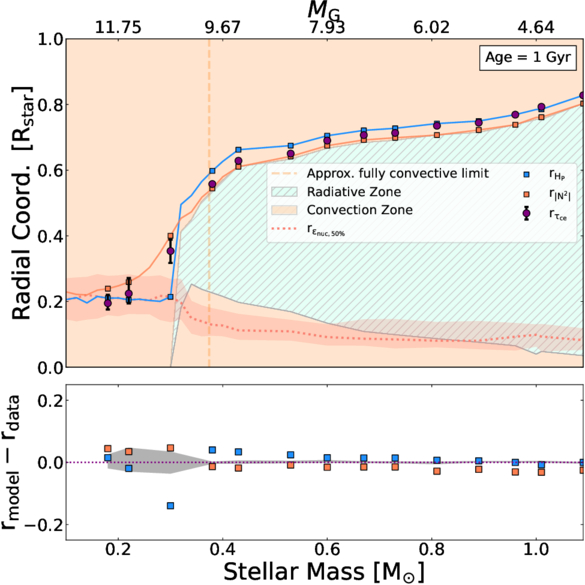
Figure 7. The radial coordinates (where zero represents the stellar center, and one the surface) of several physical quantities identified to correlate with τcE and τcE itself are plotted for each modeled stellar mass in this study. Error bars correspond to the gray regions of Figure 5. The bottom panel shows residuals for the radial coordinate between the empirical and model values, with colors corresponding to the legend. See Section 4.1 for further details.
Download figure:
Standard image High-resolution image4.1.1. The Brunt–Väisälä Frequency and Flux Emergence
The Brunt–Väisälä or buoyancy frequency is a quantity describing the frequency of oscillation for a particle displaced in a stable medium. It also serves as an indicator of convective stability in stellar atmospheres. As defined in MESA (B. Paxton et al. 2013), it may be calculated as

where B is a quantity accounting for composition gradients, as described in Section 3.3 of that text. The terms χρ and χT represent the partial derivatives  and
and  , respectively. Hence, the Brunt–Väisälä frequency is directly related to the Ledoux criterion. When N2 takes on positive values, the frequency N is real and leads to oscillatory solutions of motion (stability). However, when N2 is negative, N is imaginary and leads to exponentially growing solutions of motion, i.e., instability. In a stellar model, N2 is positive in radiative zones and negative in convective zones.
We plot ∣N2∣ in the convective zones of our models in Figure 5 as the dark orange dashed lines. We find that a position in the stellar model ( ) where ∣N2∣ > 10−14 Hz−2 (dark orange points/vertical lines) correlates fairly well with the position inferred by τcE (purple points/vertical lines). In our higher-mass models, ∣N2∣ never gets this low, and this metric is simply placed at the minimum value in the convection zone, near 10−13 Hz−2 for early M dwarfs and 10−12 Hz−2 for models representing G-type stars. In Figure 7, this location (dark orange squares and line) tracks well with rcE.
This may offer some intuition as to what physical processes are at play in the dynamo at rcE. This condition suggests that the Brunt–Väisälä growth rate for exponential motion (via unstable buoyant forces in the convection zone) should rise above a threshold before magnetic flux is efficiently transported by convection. Below this threshold, the buoyant force would grow at a rate such that it is overwhelmed by the Coriolis force, and magnetic flux rises with a trajectory emerging at relatively high latitudes. The values cited above for ∣N2∣ that are found to correlate with rcE are close to those calculated by S. D’Silva (1995). For a solar-type star, S. D’Silva (1995) analytically calculated that ∣N2∣ should be greater than 10−12 Hz−2 for magnetic flux tubes to rise exponentially in an adiabatic medium and arise at surface latitudes in agreement with sunspots. Those authors derive a condition for threshold values of ∣N2∣ that would scale with mass and could potentially provide a viable alternative approximation for defining where τc(r) should be calculated, but is beyond the scope of this work.
The concept of buoyantly rising flux tubes has undergone significant evolution over the last several decades, as reviewed by Y. Fan (2021). Initially, these models tended to consider magnetic flux being stored and rising from a stable overshoot layer beneath the convection zone and rising to become amplified by rotational shear at the tachocline. As also reviewed by P. Charbonneau (2020) and R. H. Cameron & M. Schüssler (2023), such interface dynamo models face a number of challenges, and currently produce results in contention with solar observations. Our results, like those of N. J. Wright et al. (2018), suggest that the stellar dynamo may be similar in partially and fully convective stars, the latter of which the tachocline is absent in. If the dynamo is situated deep in the CE, as suggested by our findings, then our results lend some evidence to the possibility of a global dynamo operating in the convection zone itself. Our results would also roughly align with findings from C. P. Bice & J. Toomre (2023) that suggest that a global dynamo may form a reservoir of magnetic flux tubes deep in the convection zone of both partially and fully convective stars, from which these tubes may rise to form active regions on the stellar surface.
Such models are in the vein of those described by, e.g., N. J. Nelson et al. (2011, 2013, 2014), L. Jouve et al. (2013), and Y. Fan & F. Fang (2014) where shear via turbulent convection may produce magnetic flux tubes, without the need of shear at the tachocline. These simulations tend to find magnetic flux concentrated near the bottom of the CE, which rises to form active regions at the stellar surface. Such simulations are capable of reproducing many observed properties of the solar magnetic field and bypass the difficulties encountered by interface dynamo models. They are however computationally challenging, requiring high spatial resolution to investigate further, as achieved by, e.g., H. Hotta et al. (2016) and H. Hotta & H. Iijima (2020). Further advancements will be necessary to confirm whether these models can accurately reproduce the solar cycle, and better understand details such as where fields are generated.
4.1.2. Nuclear Energy Generation Rate
Both rcM and  begin to settle at about 20% of the stellar radius in fully convective stars, suggesting the dynamo in these stars sits at a fixed fraction of the total stellar radius. Simulations by M. K. Browning (2008) suggest that convection operates relatively weakly in the centers of fully convective stars, perhaps consequently leading to relatively weak dynamo action there as well. Simulations by C. P. Bice & J. Toomre (2023) also show that the energy available to convection drops below about 0.4 R⋆ due to the rise in heating associated with nuclear burning toward the core. Thus, downward advected magnetic fields tend to collect near where this drop off occurs. Motivated by this, we examined a third metric based on the nuclear energy generation rate, in this case due to the proton–proton (p–p) chain reaction (the dominant nuclear reaction in low-mass main-sequence stars).
The pink shaded region in Figure 5 shows where the specific nuclear energy generation rate (pp) falls below 50% of its maximum value. In the outer convection zone of stars with M⋆ > 0.3 M⊙,
pp is negligible and far from this threshold; however, in fully convective stars with M⋆≤ 0.3 M⊙, one may see this boundary more clearly as the core comes into view, with
pp peaking at the center of the stellar model.
In Figure 7, we plot the metric  , which is the point at which the distribution rises to 50% of its peak value, as the dotted pink line. The shaded region in this case represents the region that spans where the distribution falls from 70% (closer to the center,
  ) to 50% (closer to the surface,
  ) of its peak value. We find that the metric
  correlates fairly well with the location of the empirical turnover times in Figure 7, roughly agreeing within errors.
We note that the nuclear energy generation metric is flat in the radial coordinate for M < 0.3 M⊙, similar to the pressure scale height metric. Conceivably, a metric based on the bottom of the convection zone and some number of pressure scale heights ≳1, as commonly used, could provide similar results for M < 0.3 M⊙, in agreement with empirical values.
4.1.3. Relative Convective Luminosity
Since the α-effect in an elementary αΩ dynamo depends on convection, it might also be expected that dynamo action is not effective where convection is weak. We examined as a function of depth the ratio of convective to total luminosity, Lc/L, for the range of masses in our study. For masses M⋆ > 0.3 M⊙, the empirical turnover times consistently occur where the ratio of convective to total power is Lc/L ∼ 0.35, confirming that dynamo action does not appear to be associated with zones of weak convection. However, at the lowest masses, Lc/L does not reach as low as 0.35 throughout the envelope, rendering any metric for dynamo action based on Lc/L problematic to apply.
4.2. Data–Model Mismatches
Several factors likely contribute to the mismatches seen between our model τcM and empirical τcE. In particular, these can be seen near the peak of τc (at about 0.3 M⊙) in Figure 3. Here, we mention and briefly discuss several possibly contributing factors: the time evolution of the convection zone, the MLT of convection, and data biases.
Throughout this work, we have assumed an age of 1 Gyr for our MESA models, essentially to ensure models (representing field stars, as appropriate for our empirical data) are on the main sequence. In reality, field stars likely exhibit a range of ages (possibly with a majority being 1−8 Gyr old, e.g., M. Fouesneau et al. 2019; D. Qiu et al. 2021). While the convective turnover time is typically not expected to evolve appreciably during the main sequence, there are nonetheless variations that can occur, affecting both stellar structure and consequently derived values of τcM, as displayed in Figure 8. Here, we constructed a high-resolution grid of MESA models in the span of 0.08–1.3 M⊙, evolved for 14 Gyr to examine the time evolution of τcM and the stellar structure in more detail. It becomes evident that, once stars have reached the main sequence, their convective turnover times roughly stabilize before increasing again when reaching the RGB.
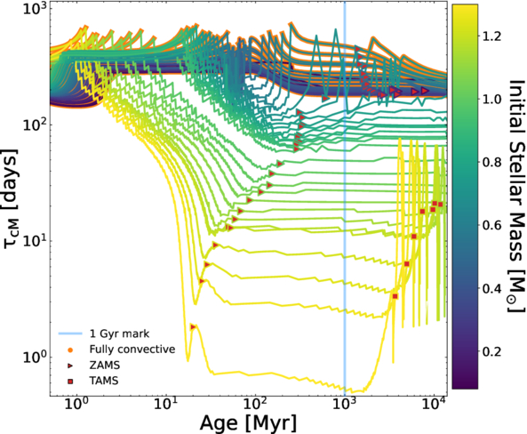
Figure 8. The time evolution of the MESA calculated convective turnover time, τcM (Section 2.2). Line colors correspond to stellar masses ranging from 0.08 to 1.3 M⊙. Red triangles indicate the zero age main sequence (ZAMS), and squares the terminal age main sequence (TAMS) as defined in A. Dotter (2016). Orange highlights indicate periods of fully convective structure. An age of 1 Gyr is marked with the vertical blue line for reference.
Download figure:
Standard image High-resolution imageIn Figure 9, we display the CE size (left panel) and central 3He (right panel) as functions of time. We note the periodic fluctuations in convection zone size, which, as shown in the right panel of Figure 9, correspond to a periodic rise and fall of central 3He. Stars in a subrange of masses within about 0.3–0.4 M⊙ may undergo an instability (dubbed the “convective kissing instability” by J. L. van Saders & M. H. Pinsonneault 2012; but see also I. Baraffe & G. Chabrier 2018) that causes the CE of these stars to periodically connect and disconnect from its convective core, due to nonequilibrium 3He burning. The exact subrange of stellar masses predicted to exhibit this behavior is model dependent, but in our case, it is exhibited by models in the range of roughly 0.31−0.33 M⊙, which is highlighted in Figure 9. Over time, one may see from Figures 8 and 9 that the peak feature of τc versus mass will change slightly with time, as the CEs of these stars connect with their convective cores. Notably, near 0.3 M⊙, our models exhibit a fairly large variation in CE size, and consequently in τcM with time, near 1 Gyr. This fact could also contribute to why our models (corresponding to individual stellar masses) predict a larger peak τcM when compared to the empirical τcE, which are a product of fits to empirical data collated in mass bins. Further, Figures 8 and 9 show that the peak should become less prominent over time as the thermal structure of stars in this mass range relaxes.
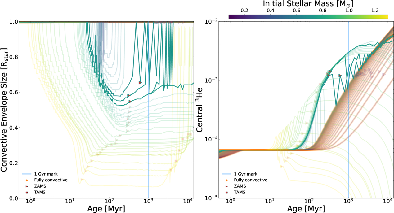
Figure 9. The time evolution of the CE size (CE size, left panel) and central 3He (right panel) for a range of stellar masses from our MESA models. Plot elements are otherwise as in Figure 8. Models in the mass range 0.31−0.33 M⊙ exhibiting the convective kissing instability (J. L. van Saders & M. H. Pinsonneault 2012; I. Baraffe & G. Chabrier 2018) leading to relatively dramatic variability in CE size are given greater visibility.
Download figure:
Standard image High-resolution imageAs our observed sample of stars likely exhibits a range of ages, rather than the 1 Gyr we compare to in our modeling, we may then expect some discrepancies to arise due to contamination from evolved stars at the high-mass end, and phenomena like the convective kissing instability near the fully convective limit. In addition, as can be seen in Figure 2, our sample of stars in the mass bin 0.25−0.35 M⊙ (with a median mass of 0.3 M⊙) is primarily comprised of stars in the magnetically saturated regime. This mass bin corresponds to the maximum of the peaked feature of Figure 3. Thus, with a greater sampling of stars in this mass range, we may see slight shifts in the peak feature of τcE. Furthermore, as discussed by F. Chiti et al. (2024), additional variations on the rotation period measurements of these stars could arise from variable starspot fractions.
A spot covering fraction could also affect the estimation of masses and effective temperatures from photometry. Starspots make the star look fainter than may be expected, thus yielding a smaller mass estimate. This effect would generate contamination in our mass bins from tending to shift stars into lower-mass bins, which would make the feature at 0.3 M⊙ smaller. Therefore, although spots could modify the mass estimates of our main-sequence stars, they do not modify our conclusions. A full analysis of the effect of spots on stellar parameters is outside the scope of this paper. If the reader wishes to estimate convective turnover times using effective temperature, we suggest using the M. J. Pecaut & E. E. Mamajek (2013) relations17 using the color (V − Ks), which is less affected by spots (L. Cao & M. H. Pinsonneault 2022).
Lastly, the theory surrounding the convective turnover time, i.e., MLT, is a 1D approximation of convection, which is in principle a 3D phenomenon in reality. As reviewed by M. Joyce & J. Tayar (2023), MLT may be considered a relatively successful theory, but it ultimately relies on parameters like αMLT that vary study-to-study (typically in the range of 1−2). With such uncertainty in MLT, precisely predicting where, e.g., the onset of full convection occurs, combined with some of the uncertainty discussed above, presents a challenge. This is especially the case considering that the mass range over which full convection takes hold (and presumably where the peak in τcE occurs) is predicted to be fairly narrow by our models (see Figure 4).
4.3. In the Context of Detailed Dynamo Models
Our findings suggest that the stellar dynamo tends to lie deep within the CE of a star. However, recent detailed simulations, such as those of G. M. Vasil et al. (2024), suggest that solar-like dynamos may viably originate in near surface shear layers (NSSL), perhaps in the outer 5%−10% of the star. It is demonstrated that rotational shear feeding the magnetorotational instability (MRI) in these outer layers can replicate torsional oscillations (H. B. Snodgrass & R. Howard 1985; S. V. Vorontsov et al. 2002) and subsurface magnetic field amplitudes (C. S. Baldner et al. 2009) detected by helioseismology. Thus, the MRI may provide a viable mechanism in the NSSL that drives the global magnetic dynamo.
As reviewed by R. H. Cameron & M. Schüssler (2023), the NSSL dynamo, or surface flux transport (SFT) models are founded on various solar observational constraints (see also the review by A. Brandenburg 2005). As mentioned in those works, a key component of NSSL/SFT models is the process of turbulent pumping within the convection zone. Arguments against NSSL dynamos had suggested that (poloidal) magnetic flux tubes rising to the surface become highly buoyant toward the stellar surface, leading to the possibility that magnetic flux may leave the NSSL before it can be amplified by shearing (A. R. Yeates et al. 2023). Simulations have found that turbulent pumping, where convective downdrafts preferentially transport magnetic flux loops downwards, may counteract this effect, leading to a concentration of magnetic energy near the bottom of the convection zone (see, e.g., Z. Zhang & J. Jiang 2022).
Bringing the discussion back to the Rossby–activity relation discussed in the present work, the Rossby number, Ro = Prot/τc, quantifies the ratio of magnetic field generation (via shear) to diffusion (via turbulent motion). In this context, our results suggest that the relevant timescale for magnetic diffusion in the dynamo is that of convection near the bottom of the convection zone. As simulations suggest that the bulk of magnetic energy may become concentrated near the bottom of the convection zone as well (N. J. Nelson et al. 2011, 2013, 2014; L. Jouve et al. 2013; Y. Fan & F. Fang 2014), τc may then correlate with the timescale on which this concentrated energy is brought toward the surface shear layers.
Many studies have approached the problem of dynamos in fully convective stars (e.g., W. Dobler et al. 2006; M. K. Browning 2008; R. K. Yadav et al. 2015, 2016; C. P. Bice & J. Toomre 2020, 2023; B. P. Brown et al. 2020). Of particular note for the work in hand, M. K. Browning (2008) presented 3D MHD simulations of the interior of a fully convective 0.3 M⊙ M dwarf. They found that fully convective stars could generate magnetic fields of kG strength, and that the field was in a rough energy equipartition with the convective flows. They also found that the amplitudes and size scales of convective flows varied strongly with the radius, with the deep interior convection being comparatively weak. Indeed, the magnetic energy density in their highest-resolution model was weak over the inner 30% of the star. Simulations from C. P. Bice & J. Toomre (2023) suggest fully convective stars may produce magnetic loops through the convection zone, with many collecting in the deep interior before rising to the stellar surface.
Recent studies have found that fully convective stars may often host dipolar magnetic field geometries, as in V. See et al. (2020) and as suggested by Y. L. Lu et al. (2024; see also a review by O. Kochukhov 2021). The fact that we find dynamo action correlated with the deep stellar interior in this work may corroborate this. As explained in M. K. Browning (2008), simulations of the geodynamo show that slower convection (larger τc) leads to a stronger influence of rotation on the dynamo. This in turn can lead to magnetic fields generated on larger spatial scales with a larger dipole fraction (see also U. R. Christensen & J. Aubert 2006; P. Olson & U. R. Christensen 2006; B. Sreenivasan & C. A. Jones 2006 for the work on planetary dynamos). Our results suggest that this will tend to be the case for fully convective stars, according to such findings. This is also found in simulations by C. P. Bice & J. Toomre (2023) of fully convective stars that tend to show greater dipole fractions in their magnetic fields. Ultimately, though, this will depend on the rotation rate of the star as well. The nature of fully convective dynamos and the fields they generate is still an active area of research. For instance, simulations by B. P. Brown et al. (2020) found that such stars may produce hemispheric magnetic field topologies, with strong implications for exoplanet habitability and stellar spin-down. We look forward to the continuing work in this area being done to improve our understanding of convection and its role in the dynamo under more realistic physical scenarios than the simplified assumptions allowed by MLT.
4.4. Implications for Stellar Spin-down
Y. L. Lu et al. (2024) found evidence that partially and fully convective stars follow starkly different spin-down laws, with fully convective stars appearing to lose angular momentum roughly twice as fast as partially convective stars for a given rotation rate, possibly due to a different dynamo mechanism. Using stellar models, F. Chiti et al. (2024) showed that the peak in τc that occurs at the fully convective boundary can explain the sharp rise observed in the rotation periods of stars at the boundary. Our results lend further observational and theoretical evidence to this possibility. Our results also corroborate the findings of F. Chiti et al. (2024) in the sense that an alternate dynamo mechanism may not be required to explain the observations described by Y. L. Lu et al. (2024). Rather, the dynamo mechanisms between fully and partially convective stars may be similar.
Another major issue in the study of stellar spin-down is that of stalling (M. A. Agüeros et al. 2018; J. L. Curtis et al. 2019, 2020). This stalling is mass dependent, where lower-mass stars stall at later times. In particular, J. L. Curtis et al. (2019) showed that stars roughly in the mass range 0.4−0.8M⊙ appear to spin-down inefficiently (stall) between the ages of about 670−1000 Myr; following the stall, stars resume relatively efficient spin-down in a similarly mass-dependent fashion (J. L. Curtis et al. 2020). In fact, standard magnetic braking models have been shown to overestimate the spin-down of stars in this mass range (e.g., S. Gossage et al. 2021), indicating a departure from standard spin-down models.
Understanding the physical mechanism(s) behind the stall is of great interest and remains a mystery. Phenomenological core–envelope coupling models have proven to successfully replicate stalling (e.g., see F. Spada & A. C. Lanzafame 2020), but a complete physical picture has yet to form. Internal gravity waves and magnetic fields (C. Charbonnel & S. Talon 2005; P. Eggenberger et al. 2005; P. A. Denissenkov et al. 2010; G. Somers & M. H. Pinsonneault 2016) have been proposed as coupling mechanisms (in the context of a related issue, lithium depletion). On stalled stars, a recent analysis by L. Cao et al. (2023) has found signatures of enhanced magnetic activity in their spectra. They suggest that a shear induced dynamo, perhaps associated with core–envelope coupling, could drive this enhanced activity.
Our new findings on τc probably do not change the story here: our findings in the mass range relevant to this topic—0.4−0.8M⊙—differ relatively slightly compared to previous studies. We note that our models predict a convective core in these models, still present at an age of 1 Gyr, that subsides over time. The presence of this core is associated with the presence and burning of 3He, which, as seen in Figure 9, becomes sharply depleted for most models following 1 Gyr (although this is mass dependent). Further investigation of whether the presence of this structure and its nature may be connected to the stalled spin-down phenomenon would be necessary to comment further.
5. Conclusions
We have empirically estimated convective turnover times from a compilation of 1451 stars with measured X-ray/bolometric luminosities from the literature (N. J. Wright et al. 2011, 2018; P. Gondoin 2012, 2013; B. Stelzer et al. 2016; N. J. Wright & J. J. Drake 2016; E. González-Álvarez et al. 2019; D. Pizzocaro et al. 2019; E. Magaudda et al. 2020, 2022; A. Núñez et al. 2022; Y. Shan et al. 2024; K. G. Stassun & M. Kounkel 2024). Using Bayesian analysis, similar to N. J. Wright et al. (2018), we empirically determined convective turnover times for stars across the mass range 0.1−1.2 M⊙. Our empirically derived turnover times show a new feature not found in previous works such as N. J. Wright et al. (2018) using the piecewise LX/Lbol–Ro relations of N. J. Wright et al. (2011).
With the data compiled in this work, we find several features in the activity–Rossby relationship that are new compared to N. J. Wright et al. (2018). We find a decrease in τc toward 1.3 M⊙, associated with decreasing CE size. We also find a sharp rise in the empirical turnover time, seeming to correspond to the stellar mass range where stars become fully convective. We find that theoretical calculations of the convective turnover time, based on MLT, roughly reproduce this feature. Using calculations from MESA r11701 stellar models, we examined the theoretical stellar structure corresponding to this feature and why it arises in both the empirical and theoretical values. Our calculations are based on a convective turnover time calculated one-half of a pressure scale height above the bottom of the convection zone, τcM (see Section 2.2.2).
Our models suggest that this feature is caused by the sudden deepening of the convection zone as a fully convective structure sets in. This causes a sharp rise in convective turnover times as the bottom of the convection zone plunges toward the stellar core. A subsequent fall in convective turnover time is also seen in both theoretical and empirical values. Our models suggest that this is due to the location of convective motion strongly influencing the dynamo and resultant magnetic activity now being fixed at roughly 20% R⋆, near the core. Meanwhile, the stellar radius shrinks with decreasing stellar mass, effectively allowing buoyancy to become stronger at this position, and τcM to shrink toward masses lower than about 0.3 M⊙.
Our results are qualitatively in agreement with those of F. Chiti et al. (2024) regarding the trend of τc with mass. It is likely that other 1D stellar evolution models would display similar behavior, subject to similar uncertainties discussed in Section 4.2, especially surrounding the treatment of convection in 1D models. For instance, the convective kissing instability occurs in a slightly narrower mass range in our modeling than it does in the modeling by J. L. van Saders & M. H. Pinsonneault (2012), ultimately impacting, e.g., the theoretical onset of fully convective structure. Future studies could be dedicated to exploring these uncertainties in more depth, and demonstrating the impact of variable chemical composition and rotation rate on convection zone properties.
This work lends support to the possibility that the magnetic dynamos of stars with 0.1 < M⋆ ≤ 1.2 M⊙ may operate similarly. At least, here, it is suggested that dynamo action driving magnetic activity measured by LX/Lbol associated with convection is seated deep within the outer convection zone, even when the star becomes fully convective (in which case it is near, but above, the stellar core). Our results are consistent with simulations suggesting that the bulk of magnetic energy may become concentrated near the bottom of the convection zone (A. Brandenburg 2005; Y. Fan & F. Fang 2014; N. J. Nelson et al. 2014; Z. Zhang & J. Jiang 2022; C. P. Bice & J. Toomre 2023; R. H. Cameron & M. Schüssler 2023). This further corroborates evidence found by N. J. Wright et al. (2018) that suggests partially and fully convective stellar dynamos have similar mechanics. Likewise, this corroborates results from simulations (e.g., A. Muñoz-Jaramillo et al. 2009; B. P. Brown et al. 2010; N. J. Nelson et al. 2013; Y. Fan & F. Fang 2014; R. K. Yadav et al. 2016; H. Hotta & H. Iijima 2020) that fully convective stars may be capable of operating a dynamo similar to partially convective stars, operating throughout the convection zone.
Acknowledgments
We extend warm thanks to Jan Eldridge for insights and discussion regarding the Eggleton pressure scale height formula. We also thank the anonymous referee for the helpful comments in improving this manuscript. S.G. acknowledges funding from Northwestern University through a CIERA Postdoctoral Fellowship and the Gordon and Betty Moore Foundation (PI Vicky Kalogera, project Nos. GBMF8477 and GBMF12341). R.K. was supported in part by the Simons Foundation (668346, JPG). K.M. was supported by NASA Chandra grants GO8-19015X, TM9-20001X, GO7-18017X, and HST-GO-15326. A.A.M. was supported by NSF Graduate Research Fellowship, grant No. DGE1745303. We would also like to thank Bill Paxton and the MESA community for making the stellar evolution code on which this work is based. This work has made use of data from the European Space Agency (ESA) mission Gaia (https://www.cosmos.esa.int/gaia), processed by the Gaia Data Processing and Analysis Consortium (DPAC, https://www.cosmos.esa.int/web/gaia/dpac/consortium). Funding for the DPAC has been provided by national institutions, in particular the institutions participating in the Gaia Multilateral Agreement.
Facilities: This research was supported in part through the computational resources and staff contributions provided for the Quest high performance computing facility at Northwestern University, which is jointly supported by the Office of the Provost - , the Office for Research - , and Northwestern University Information Technology. -
Software: MESA r11701 (B. Paxton et al. 2019); scipy (P. Virtanen et al. 2020); numpy (C. R. Harris et al. 2020); matplotlib (J. D. Hunter 2007); astropy (Astropy Collaboration et al. 2013, 2018, 2022); emcee (D. Foreman-Mackey et al. 2013).
Footnotes
- 11
Data and MESA files: https://zenodo.org/records/15680676.
- 12
- 13
See Gaia DR2 documentation (https://gea.esac.esa.int/archive/documentation/GDR2/Gaia_archive/chap_datamodel/sec_dm_main_tables/ssec_dm_ruwe.html).
- 14
- 15
Data and MESA files: https://zenodo.org/records/15680676.
- 16
Prot may nominally be considered a function of position as well, but is typically measured at the stellar surface and taken to be as such in modeling.
- 17