Abstract
We have developed a general statistical procedure for analysis of 2D and 3D finite patterns, which is applied to the data from recently released Gaia-ESA catalog DR2. The 2D analysis clearly confirms our former results on the presence of binaries in the former DR1 catalog. Our main objective is the statistical 3D analysis of DR2. For this, it is essential that the DR2 catalog includes parallaxes and data on the proper motion. The analysis allows us to determine for each pair of stars the probability that it is the binary star. This probability is represented by the function  depending on the separation. Furthermore, a combined analysis of the separation with proper motion provides a clear picture of binaries with two components of the motion: parallel and orbital. The result of this analysis is an estimate of the average orbital period and mass of the binary system. The catalog we have created involves 80,560 binary candidates.
Original content from this work may be used under the terms of the Creative Commons Attribution 3.0 licence. Any further distribution of this work must maintain attribution to the author(s) and the title of the work, journal citation and DOI.
1. Introduction
In this paper we analyze the recent data from the new catalog DR2 Gaia Collaboration et al. (2018) obtained by the Gaia-ESA mission. If compared with the previous DR1 catalog Gaia Collaboration et al. (2016a, 2016b), the DR2 contains the cleaner data complemented with parallaxes and data on the 2D proper motion. Parallaxes allow us to determine the distance of the stars, so we can substantially enlarge our former DR1 analysis (Zavada & Píška 2018) and work with the 3D patterns of moving stars.
In the present study, we focus on the statistical analysis of the presence of binaries. This topic is related to the recent studies of various aspects of binaries with the use of the catalogs DR1 (Oelkers et al. 2017; Oh et al. 2017) and DR2 (Ziegler et al. 2018; Jiménez-Esteban et al. 2019). These authors, apart from their own results, present an up-to-date overview of important findings on binary stars. Other important papers exploring wide binaries can be cited from the era before Gaia, for example, Caballero (2009) and Close et al. (1990). However, our approach and objectives are rather different, so the results obtained are complementary.
Methodology for 2D analysis has been described in detail in our above-quoted paper. In Section 2 we repeat its essence and perform generalization for the 3D case. For 2D analysis in Section 3 we take the same region in the DR2 catalog as we used in the DR1, so we can compare results from both corresponding data sets.
Principal results are obtained from the 3D analysis of a sample of DR2 data and are presented in Section 4. This part deals with two issues: the analysis of 3D separations and the analysis of proper motion of pairs of sources. The combination of both insights provides essential information about the statistical set of binaries. Obtained results are discussed in Section 5. Here we define the probabilistic function β(Δ), which is important for discussion on the occurrence of binaries. Our present catalog of binary candidates is described in Section 6, where we also shortly discuss its content and overlap with the catalog JEC—Jiménez-Esteban et al. (2019).
A brief summary of the paper is presented in Section 7. The Appendix is devoted to the derivation of some relations important for our statistical approach. The most important are distributions of separations of random sources uniformly distributed inside circles or spheres of unit diameter. The significant role of these functions for our approach is explained in Section 2.
2. Methodology
The methods are designed for analysis of the distribution of stars inside circles or spheres covering the chosen region of the sky, as sketched in Figure 1. These 2D and 3D star patterns are called events. Input data for the generation of the event grids are supposed in the galactic reference frame. So, the position  of a source is defined by spherical coordinates L, l, and b (distance from the Sun, galactic longitude and latitude):

In the center of circles or spheres we define a local orthonormal frame defined by the basis:

where  defines angular position of the event center. Unit vector kl is perpendicular to kr and has direction of increasing l, see Figure 2. Unit vector kb is defined as
  and has direction of increasing b. Vector kr has radial direction, perpendicular vectors kb and kl lies in the transverse plain.
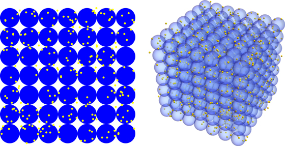
Figure 1. Grids of 2D (left) and 3D (right) events with uniform distributions of the stars.
Download figure:
Standard image High-resolution image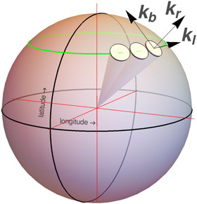
Figure 2. Galactic reference frame defined by galactic longitude and latitude with an event local frame defined by orthonormal basis kr, kl, kb.
Download figure:
Standard image High-resolution image2.1. Definition of Events
The 2D event of the multiplicity M is a set of stars with angular positions ni inside a circle with the event center n0 and a small angular radius ρ2:

With the use of event local basis (2), the local coordinates are defined as

We define the 2D event as the set:

Since the DR2 catalog involves also data on parallaxes, we can similarly also generate the 3D events—patterns of the M sources with position Li inside the spheres with the center L0 and radius ρ3:

With the use of the star positions (1) and local basis (2) we define local coordinates {Xi, Yi, Zi} as


where pi is parallax, and Li is distance of the star. The 3D event is defined as the set:

2.2. 2D Methods
The first method is based on the Fourier analysis of 2D events, where we have introduced characteristic functions Θn(M) depending on the event multiplicity M. These functions are generated by a set of events and measure statistical deviations from uniform distribution of stars  , for instance a tendency to clustering
  or anticlustering
  . Details of the method are described in Zavada & Píška (2018), in this paper we will present only the result.
With the use of a second complementary method, we analyze distributions of angular separations of sources inside the 2D events (5). Distribution is generated from the set of events. We use either absolute separations

or scaled ones

The suitable unit of the parameters xi, yi, ρ2 will be for our purpose 1 as (1″). Distribution of scaled separations generated by Monte Carlo (MC) for a uniform distribution of stars in the sky is shown in Figure 3. The exact shape of normalized MC distributions reads


where the functions EllipticK (EllipticE) are complete elliptic integrals of the first (second) kind. The proof is given in the Appendix. These distributions do not depend on the event multiplicity and radius, this is an advantage of the scaled separations. Obviously, we have always  . These exact functions replace their approximations resulting from the MC calculation applied in the previous paper.
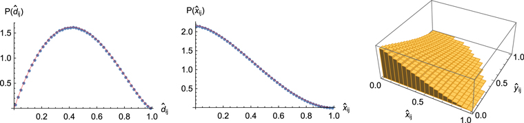
Figure 3. MC distributions of separations of uniformly generated stars (points). The red curves represent the functions (12) and (13). The MC statistics correspond to 5 × 10⁵ events of multiplicity M = 5.
Download figure:
Standard image High-resolution image2.3. 3D Methods
Similarly, as in the 2D case, we shall work with absolute separations


and/or with the scaled ones
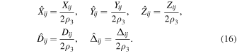
The suitable unit of the parameters Xi, Yi, Zi, ρ3 is for our purpose 1 pc. Distribution of scaled separations generated by MC from the uniform distribution of stars in the 3D region of the sky is shown in Figure 4. Exact shapes of these normalized MC distributions read

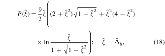

as proved in the Appendix. Shapes of these distributions similarly to (12) and (13) do not depend on event multiplicity and radius. The analysis with the use of characteristic functions Θn(M) could be in the 3D case done separately in the plains XY, YZ, and ZX. However, such analysis is not the aim of the present paper.

Figure 4. MC distributions of separations between uniformly generated stars (points) in 3D. The red curves represent functions (17)–(19). The MC statistics is represented by 5 × 10⁵ events of multiplicity M = 5.
Download figure:
Standard image High-resolution image2.4. Aims
In Section 3 using the DR2 data set we shall obtain the characteristic functions Θn(M), afterwards we check distributions (12) and (13). The distributions (17)–(19) will be used for the data analysis in Section 4.1. All these distributions are of key importance for the analysis of real data. They represent the templates, which can reveal a violation of uniformity in the star distributions. Binary (and multiple) star systems are an example of such a violation, which manifests as the peaks in the distributions of angular or space separations in the region of close sources. In general, the scale of expected structure violating uniformity should be less than the event radius ρ2 or ρ3.
3. Analysis of 2D Events
Here we present the results obtained from regions of the DR2 catalog listed in Table 1. The regions are shown in Figure 5. The corresponding events are created with the same angular radius as in Zavada & Píška (2018), which allows us the consistent comparison of results from the DR1 and DR2 catalogs. First, we checked the events covering the regions N and S. Their nonuniformity defined by the characteristic functions Θn(M) is demonstrated in Figure 6. The clear result Θn(M) > 1 indicates the presence of clustering.
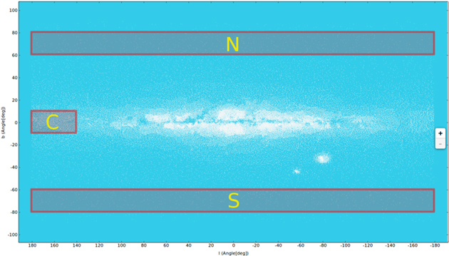
Figure 5. Analyzed regions in the DR2 catalog.
Download figure:
Standard image High-resolution image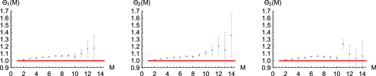
Figure 6. Characteristic functions Θn(M), n = 1, 2, 3 for events in the area N and S without any cut on magnitudes. Red line corresponds to the uniform distribution of sources.
Download figure:
Standard image High-resolution imageTable 1.
Analyzed Regions in the DR2 Catalog, Where ρ2 Is the Angular Radius of the Events,  Are Average Distance and Event Multiplicity, and Ne Is the Total Number of Events
| 2D Region: l × b(deg2) | ρ2(as) |

|

|
Ne | |
|---|---|---|---|---|---|
| N and S |

|
72 | 1290 | 3.21 | 2055,674 |
| C |

|
18 | 1912 | 2.75 | 3588,183 |
Note. Only sources in distance 1–5000 pc are taken into account. The analysis is done for events 2 ≤ M ≤ 15.
Download table as: ASCIITypeset image
Corresponding distributions of angular separations are shown in Figure 7 together with curves (12) and (13). These results can be compared with those in Figures 7 (lower panels), 10, and 11 in the former paper. We observe:
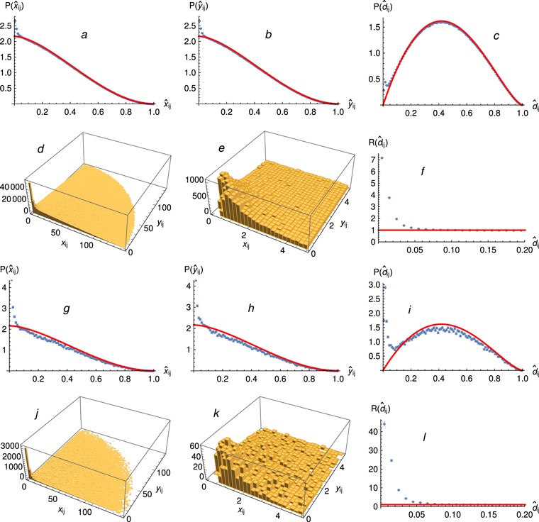
Figure 7. Panels (a)–(f): distributions of angular separations in the region N and S for all G. The blue points in the panels (a)–(c) represent the data on scaled separations  and the red curves are functions (12) and (13) representing uniform simulation. Panel (f) is the ratio of data to simulation from panel (c). Panels (d) and (e) represent 3D plot of separations xij, yij in different scales (unit is 1 as). Panels (g)–(l): the same for sources G ≤ 15.
Download figure:
Standard image High-resolution image(i) The peaks at small angular separations in the DR2 corresponding to binaries are clearer and more pronounced than in the DR1 catalog. Panels (e) and (k) in Figure 7 demonstrate the double stars separated by  are absent because such close pairs are not resolved in the DR2 data set as reported in Arenou et al. (2018). In both catalogs, we observe an excess of binaries in the region N and S for
  or equivalently for dij ≲ 8.6 as. For greater separations inside the event, we observe perfectly uniform distributions of stars. Note the data and curves are equally normalized for
  . That is why the strong peak in panels (g)–(i) is balanced by a small reduction of distribution outside the peak. Brighter stars (G ≤ 15, panels (g)–(l)) show evidently stronger peaks than the sample without any cut on magnitude (panels (a)–(f)). A similar tendency was already observed in the catalog DR1.
(ii) A more pronounced presence of binaries is demonstrated also in Figure 6. The slopes of lines in DR2 are greater than in DR1—clustering is more obvious. For M ≤ 8 the slopes are ≈4%(8%) for the DR1(DR2) data. In Figure 8 we have shown some results obtained in a more populated region C. Also here we can observe a clear peak at small angular separations of sources of the magnitude G ≤ 15, which proves the presence of binaries. Panel (b) again demonstrates the absence of double stars separated by  due to insufficient resolution. Different scales of
  in Figures 7(l) and 8(c) are due to different radii ρ2 of events from N and S and C regions. Similar plots could be presented for whole spectrum of magnitudes in region C; however, elevation above the red line due to binaries is much less than that in Figure 8(c). The reason can be that denser region C with all magnitudes generates higher background of the optical doubles and a consequently lower relative rate of binaries.
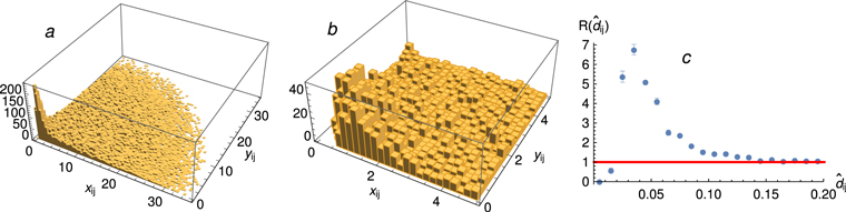
Figure 8. Panels (a)–(c): distributions of angular separations in the region C for sources G ≤ 15. Panels (a) and (b) represent a 3D plot of separations xij, yij in different scales (unit is 1 as). Panel (c) is the ratio of data distribution  to the function (12), like panels (f) and (l) in previous Figure 7.
Download figure:
Standard image High-resolution image4. Binaries in 3D Events
We present the results obtained from the 3D region defined in Table 2. The parallax and angular components of the star proper motion are the parameters, which substantially enrich the recent Gaia data. We work with the 3D events (9).
Table 2. Region of 3D Analysis is Cube Centered at the Origin of the Galactic Reference Frame
| Region |

|

|

|
Ne |
|---|---|---|---|---|
| Cube of edge 400 pc | 2 | 188 | 6.8 | 727,744 |
Note. Only sources of positive parallax are included. ρ3 is the radius of events,  are average distance and event multiplicity, and Ne is the total number of events. The analysis is done for events 2 ≤ M ≤ 15.
Download table as: ASCIITypeset image
4.1. Analysis of 3D Separations
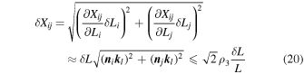
The summary results of the analysis obtained from all magnitudes G are shown in Figure 9. Distributions of scaled separations in panels (a)–(c), (g), and (h) perfectly match the uniform distribution of sources, but with the exception of the first bin in (a), (b), and (h). Apparent excess of very close pairs in planes XY, YZ, and ZX is seen also in panels (d)–(f). However, the sharp peak can be observed only in the plane XY (panel (d) and its magnified version (j)). Smearing in the direction of Z (difference of radial positions, panels (c), (e), and (f)) is due to lower accuracy in measuring of parallaxes. The errors of local coordinates depend on the errors of separations and with the use of definitions (7) and (8) are calculated as
and similarly

Note that  , where p is parallax. Obviously δZij ≫ δXij, δYij since
  . That is why we prefer distributions of Δij to Dij for obtaining precise results. Maximum values of separations X, Y, and Z is 4 pc, which follows from the event radius ρ3 = 2 pc. The excess of close pairs is obvious most explicitly from the distribution of Δij in panel (k) that represents a magnified version of (h). The important ratio of the distribution P(Δij) to the uniform simulation (red curve in panel (h) rescaled to
  ) is shown in logarithmic scale of Δij in panel (i).
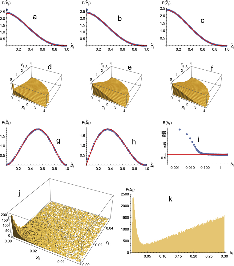
Figure 9. Distributions of separations (14)–(16) for all G. The blue points in the panels (a)–(c), (g), and (h) represent the data on scaled separations  and the red curves are functions (17)–(19) representing uniform simulation. Panels (d)–(f) show 2D projections of separations. Panel (i) is the ratio of data to simulation from panel (h). Panels (j) and (k) are magnified versions of (d) and (h). Unit of separations
  is 1 pc.
Download figure:
Standard image High-resolution imageThe same distributions but for brighter sources G ≤ 15 are shown in Figure 10. Similarly, as in the 2D case, the peaks are stronger for brighter sources and distributions outside the peaks confirm uniformity of the star distribution. Again due to equal normalization of data and red curves for  the strong peak in panels (g) and (h) is balanced by a small reduction of distribution beyond the peak. The excess of close pairs observed in both figures again convincingly indicates the presence of binaries.
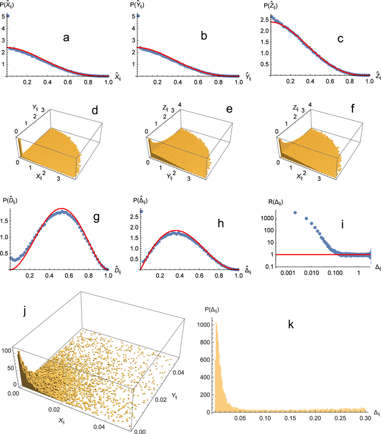
Figure 10. Same distributions as in the previous figure, but for bright pairs, G ≤ 15.
Download figure:
Standard image High-resolution imageFor quantitative estimates, the important panel is (i), which displays the ratio data/simulation. This is more accurate than only displaying peaks with some undefined background. Panel (i) suggests that separations of binary systems in the analyzed region meet very approximately

We observe only a tail of distribution corresponding to more separated binaries. Closer pairs are absent due to the limited angular resolution in DR2 data. This result is compatible with the older data reported in Close et al. (1990). In Section 5 further discussion is devoted to the probability of the binary separation above this limit. We have checked that sampling with events generated by spheres of different radius (ρ3 = 5 pc) does not change the approximate result (22).
4.2. Proper Motion of Binaries
The proper motion of the stars in DR2 is defined by two angular velocities

in directions of the R.A. and decl. in the ICRS. So the corresponding transverse 2D velocity U is given as

where L is distance of the star calculated from the parallax (8). For the pair of stars we can define:

where αij is the angle between both transverse velocities. The corresponding errors read

where

Note that relative error δvij/vij can be large, since vij is small compared with Uij and the errors  and
and  are the same. In Figure 11(a) we show the distribution of the velocities U of the stars from the region defined in Table 2. Distribution of the corresponding pair angles αij is presented in Figures 11(b)–(d) for different regions of Δij. In Figure 12(a) we have shown the correlation of pair transverse separations and angles
  . We observe a very narrow peak in the region of small Δij and
  .1
The peak is connected with presence of binaries as follows. The transverse velocities of two gravitationally coupled stars are
.1
The peak is connected with presence of binaries as follows. The transverse velocities of two gravitationally coupled stars are

where V is transverse velocity of their center of gravity and vi, vj are transverse projections of instantaneous orbital velocities, they have always opposite direction. Dominance of very small αij means that

so for binaries in our Δ window (Δmin is given by resolution of two close sources and Δmax = 0.1 pc by (22)) we have

For comparison, we have generated an MC plot from uniform distributions of positions and velocity directions, which is shown in Figure 12(b). Obviously, uniform distribution contradicts Figure 12(a), which reflects the presence of binaries (peak at small αij and  ). The corresponding αij peak is also observed in Figures 11(b)–(d) on the background of the collective motion of stars (dominance of αij < 90°). The peak is suppressed for Δij ≳ 1 pc. Selection of comoving systems is a basis of the methodology applied in the catalog JEC.
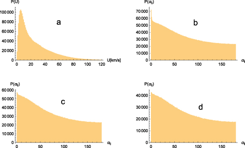
Figure 11. Panel (a): distribution of the star transverse velocities. Panels (b)–(d): distribution of the corresponding pair angles αij for  and 1 pc.
Download figure:
Standard image High-resolution image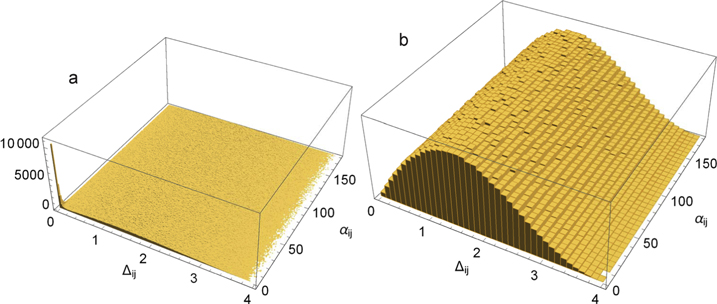
Figure 12. Panel (a): correlation of the pair transverse separation (unit is 1 pc) with angle of corresponding transverse velocities. Panel (b): corresponding MC simulation generated from uniform distributions of positions and velocity directions.
Download figure:
Standard image High-resolution imageIn Figure 13 we show correlations of the velocities V and vij with Δij in the region of small separations, where the binaries are present. With the use of vij and Δij we try to roughly estimate the orbital period of the binary star. To simplify the calculation, we assume the space binary orbits are circular and the star 3D separation is a (semimajor axis). There are the extreme cases:
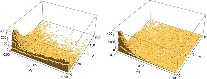
Figure 13. Correlation of the pair transverse separation Δij with the transverse velocity V of the star system and with the transverse velocity vij of periodic motion. Unit of velocity is km s−1.
Download figure:
Standard image High-resolution image(A) M1 ≈ M2, then

Orbital period is

where w is the space orbital velocity and a equals the diameter of the orbit.
(B) M1 ≫ M2, then

but the orbital period is different

since the separation a equals to the orbit radius.
At the same time, Kepler’s law implies for orbital period Tg:

where G is gravitational constant and  is mass of the star system. For units
 ![${T}_{g}\left[{\rm{y}}\right],a\left[\mathrm{pc}\right]$](https://content.cld.iop.org/journals/1538-3881/159/1/33/revision1/ajab5865ieqn40.gif) , and
, and ![${M}_{\mathrm{tot}}\left[{M}_{\odot }\right]$](https://content.cld.iop.org/journals/1538-3881/159/1/33/revision1/ajab5865ieqn41.gif) we have
we have

This relation also allows us to estimate the period. If the plane of orbit is perpendicular to the line of sight (axis Z), like the orbit N in Figure 14(a), then it is possible to simply substitute:
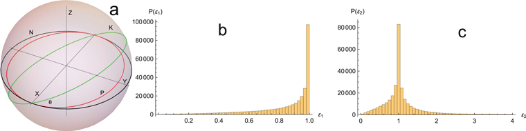
Figure 14. Panel (a): real orbit (K) and its deformed projection on the sky (P). Real orbit (N) in the plane xy. Panels (b) and (c): distributions of random parameters ε1 and ε2.
Download figure:
Standard image High-resolution image
 in (32),
  in (34) and
  in (36), (32), and (34).
Then we get:

The orbit reference frame in the figure is similar to the local 3D event frame defined by the basis (2) and coordinates (7). But its origin L0 is defined by the actual position of the center of mass of the binary. How does one deal with the orbits whose plane is not perpendicular to the line of sight like the orbit K in the same figure? The orbits in the figure are defined as follows:

where r = a/2 for the case (A), r = a for (B), and ϕ is azimuthal angle in the plane XY. The orbit K inclined at an angle θ is observed only in its projection P. Corresponding observed separation between the stars is Δij:

Random angles ϕ, θ generate distribution of ε1 shown in Figure 14(b). The MC distribution demonstrates smearing of the real separation a due to random ϕ and slope θ of the orbit. Similarly, the ratio a/w is distorted as

Since velocity w is perpendicular to r, there is exchange  in denominator. Corresponding distribution of ε2 is shown in Figure 14(c). The mean values are

and represent a scale of distortion of real orbital periods, if replaced by relations (37). More accurate estimate of the periods in some region of Δij can be obtained by rescaling of these relations:

We have estimated the average periods from the maximum in Figure 13. If we take the sources roughly in the region of half width of the maximum,

then

and one can check that equality  implies estimation Mtot ≈ 0.8 M⊙.
5. Discussion
The separation of a pair of stars and the similarity of their movements can serve as two signatures of the binaries. We can compare them:
(i) Distributions of the 2D and 3D separations are studied in Sections 3 and 4.1. The procedure is simple, the distribution of separations P(Δ) (within the defined circles or spheres) is compared with the corresponding separations Pbg(Δ) generated by uniformly distributed sources representing background

where P0 is given by (12) or (18) and Nbg is the corresponding number of the background pairs in the data events. Its accurate calculation is described below, see Equations (47)–(49). The binary distribution reads

and the probability  that the pair is a real binary is given as

The function  displayed in Figures 7(f) and (l), 8(c), 9(i), and 10(i) is another representation of the probabilistic function
  :
:

Consider the distribution  from Figures 9(k) and 10(k). The corresponding function
  is shown in Figure 15(a), where the red curve represent fit of the function:

The result of the fit is shown in the first row (all pairs) of Table 3. The longer tail corresponding to the second term describes the small probability of bound pair at greater separations: Δ ≳ 0.15 pc. This tail is not visible in panels (i) in Figures 9 and 10. Two exponential terms in  may correspond to two different classes of binaries. The question is to what extent the excess of wide binaries consists of stable bound systems. Part of the excess may be an image of widening pairs that were less separated but weakly bound in the past. The accuracy of the method is based on three conditions:
- 1.precise separation measurement in a suitably selected statistical set of events that generates
 ,
, - 2.precise modeling of the background defining Pbg(Δ), and
- 3.relatively high peak and low background giving probability close to 1 in the peak region.


(ii) In principle, a similar approach could be applied to comoving pairs. However, it is obvious that meeting the conditions above is more difficult for velocities or their differences. The precision of velocity measurement is lower than separation. The distribution of velocities is far from being simply uniform, we do not know the exact form of the velocity background. Figure 11(b) suggests a more complicated collective motion in the background and a relatively low peak of binaries. That is why we prefer the primary signature based on the spatial separation, where we work with exactly defined background and relatively high peaks, like panels (i) and (k) in Figures 9 and 10. On the other hand, one can expect that a combination of position and velocity data will suppress background and improve the selection of binaries in terms of the function  . A selection based on such a combination is described below. In Section 4.2 we have shown that combination of the space separation with proper motion allows us to estimate the orbital period.
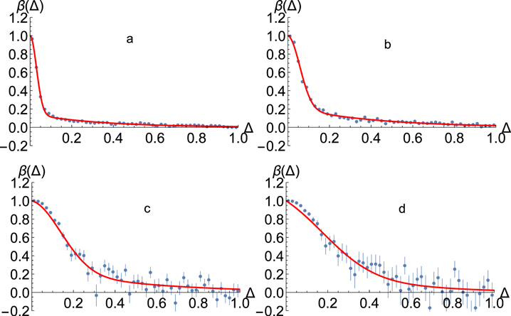
Figure 15. Probabilistic function  for different domains Δ × α and intervals of magnitude G. Panel (a): all pairs and magnitudes. Panels (b)–(d): united domain AB for magnitude intervals G all, G ≤ 15, G ≤ 13. Blue points with error bars are data, red curves are fits (46).
Download figure:
Standard image High-resolution imageTable 3. Values of the Parameters ω, σ1, σ2
| ω | σ1(pc) | σ2(pc) | |
|---|---|---|---|
| All Pairs | 0.852 | 0.335 | 0.0303 |
| All Pairs and Domain AB | 0.771 | 0.396 | 0.0573 |
| G ≤ 15 and Domain AB | 0.705 | 0.464 | 0.143 |
| G ≤ 13 and Domain AB | 0.505 | 0.326 | 0.215 |
Download table as: ASCIITypeset image
We denote by  and
and  the numbers of real and false (background) binaries in some domain D of separations Δ. Correspondingly we denote
  , where
  is the number of pairs in a given data set. We have

where Pbg is distribution defined by (18) and renormalized in such a way that

where the integration is over the domain E safely outside the peak of binaries. So we calculate

where P0 is defined by (18) with the substitution  . The same procedure can be applied for the domains
  . Since we can assume that Δ and α are not correlated in the background distribution

then

If we choose  then the second ratio is 1. In this way, we can calculate NbgD without the knowledge of
  The selected domains are shown, together with the results β ≈ Nbin/ N2 in Figure 16. For the calculation, we take the common interval
  pc, where NbinE should be zero. In accordance with Figure 12(a) we observe the highest rate of binaries in the domain
  deg. The binaries are well observable also in the neighboring domain
  deg. For G ≤ 15 the number of binaries in the domains C is zero within statistical errors. Presence of binaries in the domain D requires further analysis.

Figure 16. Ratio Nbin/N2 of the number of binaries and the total number of pairs in different domains Δ × α and intervals of magnitude G.
Download figure:
Standard image High-resolution imageThe probabilistic function  corresponding to the united domain AB is shown in panels (b)–(d) in Figure 15 for different intervals of the magnitude G. Obviously, the function (46) fitted with the parameters listed in Table 3 can be rather approximate. We observe that function β is getting wider with decreasing G. This may suggest that brighter and therefore statistically more massive stars can form stable bound systems even at greater separations. Obviously, for Δ ≳ 1 pc, the probability β is compatible with zero. This also corresponds to an absence of a binary peak in Figure 11(d), which relates to Δ > 1 pc. Total numbers of binaries are listed in Table 4. The results suggest that in the Gaia DR2 data in the region defined by Table 2, the number of binaries can represent ≈2% of all stars in this region.
Table 4. The Number of Binaries Nbin with the Total Number of Sources Ns in Different Intervals of the Magnitude G
| Ns | Nbin | Nbin/Ns | |
|---|---|---|---|
| All G | 2734,222 | 66,962 | 0.024 |
| G ≤ 15 | 474,689 | 10,781 | 0.023 |
| G ≤ 13 | 256,787 | 4405 | 0.017 |
Download table as: ASCIITypeset image
6. Catalog
In this section, we describe the catalog of binary candidates, which we have created from the events of multiplicity 2 ≤ M ≤ 15 defined by Table 2. For the first version of the catalog we accept only the candidates from domain A shown in the first panel in Figure 16. So, we do not accept all candidates, but only candidates with a high probability to be the true binary. The candidates meet the following conditions:
(1) Projection of separation
We accept the pairs, which satisfy

In general, the projection of separation Δ depends on the reference frame. In the paper, we worked with the local reference frame defined by the event center, where projection Δ into the local plane XY is given by (15). In the catalog we do not use local frames. The cut (52) is applied to Δcat, which is defined as the length of the arc

where Lα, nα are defined in Section 2.1. The separations Δ and Δcat are not exactly equal, but we have checked that in our conditions their difference is small,  pc. Then the sharp cut on
  means only a slightly smeared cut of the distribution of Δ.
(2) Projection of collinearity
The pairs must meet the condition

Both conditions define the domain A in the first panel of Figure 16. The panel shows that the average probability of a binary star is β ≈ 84%. If the stars are brighter, (second and third panel), then the average β is almost 100%.
(3) Radial separation
In fact, the radial separation is not explicitly used in our algorithm for selection of binaries. The reason is a rather low precision of radial separations, as explained in the discussion of panels (c), (e), and (f) in Figures 9 and 10. The only constraint is given by the diameter of our events (4 pc). Separation selection is based solely on Δij. Additional cuts on inaccurate radial separation would eliminate many of the real binaries and invalidate the function β calculated for Δij. We obtained high β even without a cut on radial separation.
Furthermore, it is evident that spherical events fill the space only partially (≈52%). In this way, half the stars are lost for analysis. We also lose binaries between two adjacent events when each star falls into another. In order to recover these losses, we work with the modified coverage:
- (i)
- (ii)The procedure is repeated with the same cubes centered in the corners of the former cubes and the search results are merged.
The catalog is represented by a matrix that is defined as follows. Each line represents one star and the following data are in the columns:
1–2: Group ID and Group size  to match stars with the group they belong to.2
3–96: Copy of the original entry for the star from Gaia-DR2 archive,3 according to the documentation.4
97–98: Minimum and maximum angular separation of the star from other stars in the group [as].
99–100: Minimum and maximum projected physical separation of the star from other stars in the group [pc].
The summary data from our catalog of binary candidates (I), along with the data extracted from the catalog JEC - Jiménez-Esteban et al. (2019) (II) is shown in Table 5. The number of candidates N2 in this table correspond to N2 in the domains A in Figure 16 after increasing with the repeated covering. The comparison of the two catalogs shows the following:
- (a)We can only compare sources of magnitude G ≤ 13, because (II) does not contain less bright stars. Of the total number 3055 binaries in (II), only 301 lie in the (I) cube. Increasing the edge of this cube by the factor 2.15 would increase volume 10 times with the number of binaries comparable to the total (II).
- (b)The number 301(II) could be compared with the corresponding number of candidates C2 = 9082(I). However, in the JEC catalog, apart from the cut G ≤ 13 many other restrictions and selections are made. Definition of the binary is not the same in both catalogs. In our opinion, this is the reason for the difference between (I) and (II).
- (c)(I) and (II) have 108 common binary candidates.
- (d)86(II) candidates are absent in (I) since the separation Δ exceeds 0.15 pc. These candidates do not contradict our general criteria, but the corresponding probability can be lower as shown in Figure 15.
- (e)54(II) candidates are absent in (I) since their spatial separation exceeds 4 pc (event diameter). Such candidates may not contradict our criteria; however, due to a great background can be extremely low.
- (f)18(II) candidates are absent in (I) since these candidates are located in a dense area generating the high multiplicity events, which exceed our currently set limit.
- (g)The last 35(II) candidates are absent in (I), mainly due to the fact that even after the second coverage some couples (II) remain separated in two neighboring event cubes.


Table 5. Summary Table of Binaries from the Catalogs (I) and (II), See the Text
| Catalog |

|
G |
|---|---|---|
| (I): Domain A |

|
All |

|
≤15 | |

|
≤13 | |
| (II): Total Nbin = 3055 |

|
≤13 |
Note. N2 is the number of binary candidates, Nbin is the real expected number of binaries. The data in the second column are related to the full cube region  (Table 2).
Download table as: ASCIITypeset image
The total number of the binary candidates of all Gaia magnitudes in the catalog (I) is 80,560, which corresponds to the expected real number of binaries 67,670. The full current catalog (I) in the csv form is available on the website https://www.fzu.cz/~piska/Catalogue/. We plan to further develop and optimize our catalog methodology.
7. Summary and Conclusion
We have proposed a general statistical method for analysis of finite 2D and 3D patterns. In the present study, the method has been applied to the analysis of binary star systems in different regions of the Gaia catalog DR2.
Results on 2D statistical analysis were compared with our former results obtained from the previous catalog DR1. The new results give in the distribution of angular separations more clear evidence of binaries. Independent signature follows from the characteristic functions  , which clearly indicate a tendency to clustering. However, the most important results are obtained from the 3D analysis introduced in the present paper. We have analyzed about 5 × 10⁵ of events inside the cube of edge 400 pc centered at the origin of the galactic reference frame. In distributions of pair separations, we observe the sharp peaks at small separations corresponding to binaries, which are more striking for brighter sources, G ≤ 15.
The important result of the analysis is probabilistic function  , which depends on the separation Δ of a pair of stars and indicates the probability that the pair constitutes a bound system. The function suggests that brighter, more massive binary stars have on average a greater separation. With increasing separation the function falls rapidly. We obtained the ratio binaries/singles ≈2%.
Furthermore, we had shown that a combined analysis of 3D separations with the proper motion of the pairs of sources gives a clear picture of the binaries with two components of the motion: parallel and orbital. The analysis allowed us to estimate the average orbital period and mass of the binary star system in the chosen statistical ensemble.
The highest probability of the binary is observed at smallest separations Δ and angles α between proper motions. From the corresponding domain  deg, we have created the catalog involving 80,560 binary candidates, which represents 67,670 of the true binaries.
This work has made use of data from the European Space Agency (ESA) mission Gaia (https://www.cosmos.esa.int/gaia), processed by the Gaia Data Processing and Analysis Consortium (DPAC, https://www.cosmos.esa.int/web/gaia/dpac/consortium). Funding for the DPAC has been provided by national institutions, in particular, the institutions participating in the Gaia Multilateral Agreement. The work was supported by the project LTT17018 of the MEYS (Czech Republic). Furthermore, we are grateful to J. Grygar for deep interest and many valuable comments and J. Palouš and O. Teryaev for very useful discussions and inspiring comments.
Appendix: Proof of Relations (12), (13), and (17)–(19)
(i) Relation (12)
First we consider two random points on a segment L. The probability that the points are separated by interval l reads:

Furthermore, we suppose a circle of diameter  with a chords L(y) involving random segment l (Figure 17). We have

The probability of interval l reads

This distribution is generated by random pairs on the chords parallel to axis x. For arbitrary random pairs separated by l inside the circle, we integrate distributions (57) over all directions in 2D and replace

which gives distribution

Relation (12) is its normalized form.
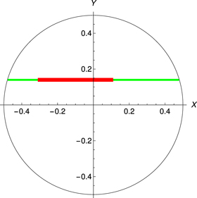
Figure 17. Random segment l (red) on the chord L(y) (green).
Download figure:
Standard image High-resolution image(ii) Relation (13)
Distribution (59) can be modified

Calculation of integral

with the use of Wolfram Research, Inc. (2019), and after replacement  and normalization gives relation (13).
(iii) Relation (17)
Now instead of circle 2R = 1, we consider the sphere of the same radius. The procedure is a modification of the case (i). Now instead of integral (57) we get
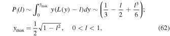
where y means radius of a cylinder of parallel chords. The additional y in the integral means that we integrate chords on surfaces of cylinders of different radii. Then instead of (58) we use

since the integration of chords is over all directions in 3D. The resulting distribution reads

which after normalization gives relation (17).
(iv) Relation (19)
Probability  of random segments
 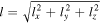 inside the sphere can be expressed as

which together with (64) gives

The probability that segment l has projection lx is given as


The last integral (equally for ly, lz) can be after inserting from (66) easily calculated, and after normalization gives relation (19).
(v) Relation (18)
In a similar way, the probability that segment l has projection  is given as

which after inserting from (66) and integration with the use of Wolfram Research, Inc. (2019) implies relation (18).
Footnotes
- 1
Input data (23) are related to the ICRS and
is calculated in the galactic reference frame. Nevertheless the parameters are invariant under rotation. - 2
In the current version of our catalog we omit candidates of systems n > 2, so only binaries (n = 2) are written.
- 3
- 4

