Abstract
We report measurements of the sky-projected spin–orbit angle for AU Mic b, a Neptune-size planet orbiting a very young (∼20 Myr) nearby pre-main-sequence M-dwarf star, which also hosts a bright, edge-on, debris disk. The planet was recently discovered from preliminary analysis of radial-velocity observations and confirmed to be transiting its host star from photometric data from the NASA’s TESS mission. We obtained radial-velocity measurements of AU Mic over the course of two partially observable transits and one full transit of planet b from high-resolution spectroscopic observations made with the Minerva-Australis telescope array. Only a marginal detection of the Rossiter–McLaughlin effect signal was obtained from the radial velocities, in part due to AU Mic being an extremely active star and the lack of full transit coverage plus sufficient out-of-transit baseline. As such, a precise determination of the obliquity for AU Mic b is not possible in this study and we find a sky-projected spin–orbit angle of  . This result is consistent with both the planet’s orbit being aligned or highly misaligned with the spin axis of its host star. Our measurement independently agrees with, but is far less precise than observations carried out on other instruments around the same time that measure a low-obliquity orbit for the planet. AU Mic is the youngest exoplanetary system for which the projected spin–orbit angle has been measured, making it a key data point in the study of the formation and migration of exoplanets—particularly given that the system is also host to a bright debris disk.
1. Introduction
Prior to the discovery of the first planets orbiting other stars, our only laboratory for the study of planet formation was the solar system. While our planetary system holds a great wealth of information on the way in which planetary systems form and evolve (as described in detail in the recent review by Horner et al. 2020), it represents just one possible outcome of that process. For that reason, the discovery of the first exoplanets (e.g., Campbell et al. 1988; Latham et al. 1989; Wolszczan & Frail 1992; Mayor & Queloz 1995) led to a revolution in our understanding of planet formation—giving our first insight into the true diversity of outcomes for the planet formation process.
One of the most startling discoveries of the exoplanet era has been that of the so-called “hot Jupiters”—giant planets moving on orbits that almost skim the surface of their host stars (e.g., Sanchis-Ojeda et al. 2015; Dai et al. 2016; Vines et al. 2019). A number of mechanisms have been proposed to explain the migration of the hot Jupiters—ranging from planet–planet scattering (e.g., Chatterjee et al. 2008; Beaugé & Nesvorný 2012) to interaction with the material within the protoplanetary disk (e.g., Lin et al. 1996; Ward 1997; Tanaka et al. 2002; Alibert et al. 2005)—and even orbital excitation by a distant companion of their host star, followed by a process of tidal circularization, locking the planet’s orbit in at the distance of its periastron passage (e.g., Wu & Murray 2003; Nagasawa et al. 2008; Nagasawa & Ida 2011; Petrovich 2015). For a review of the different processes that may play a role in the formation of hot Jupiters, we direct the interested reader to Dawson & Johnson (2018).
Distinguishing between these planet migration mechanisms is currently a leading goal of exoplanetary science. Each migration mechanism would result in a dramatically different planetary system. A variety of observational methods can come together to identify which have been active in a given system hosting a short-period planet. Of particular interest here are observations of the “Rossiter–McLaughlin effect” (McLaughlin 1924; Rossiter 1924), which allows the sky-projected inclination (obliquity) of the planet’s orbit with respect to the plane of its host star’s equator to be accurately determined. Such observations have revealed a significant population of strongly misaligned exoplanets (e.g., Hirano et al. 2011a; Addison et al. 2013; Rodríguez Martínez et al. 2020), including planets moving on retrograde orbits (e.g., Siverd et al. 2018; Temple et al. 2019).
In this context, it is particularly interesting to study planets that have only recently formed, or are in the process of formation and migration. The transiting planet orbiting AU Microscopii, AU Mic b, is a particularly interesting target in this regard. AU Mic is a young (23 ± 3 Myr; Mamajek & Bell 2014), nearby (d = 9.725 ± 0.005 pc; Gaia Collaboration 2018) M-type star (M1 V; Keenan & McNeil 1989), surrounded by a substantial, spatially resolved debris disk (e.g., Kalas et al. 2004; Liu 2004; MacGregor et al. 2013). It is known to host at least one planet—AU Mic b, which transits its host every 8.46 days (Plavchan et al. 2020). Additional planets in the system are suspected from multiwavelength radial-velocity measurements (Plavchan et al. 2020) and tentative evidence of disk substructure at millimeter wavelengths (Daley et al. 2019).
The disk around AU Mic has been imaged at a wide range of wavelengths, revealing its orientation and extent (e.g., Kalas et al. 2004; MacGregor et al. 2013; Matthews et al. 2015; Holland et al. 2017). Overall, the disk architecture is a single broad and coplanar belt oriented edge on, extending out to 210 au in scattered light (Kalas et al. 2004), with the dust-producing planetesimal belt located around 40 au from the star (MacGregor et al. 2013). Collisonal modeling of the disk suggested that the disk should be dynamically cold (Schüppler et al. 2015); recent high angular resolution ALMA observations of the disk have resolved its vertical extent, finding it to be vertically thin and unstirred, ruling out the influence of planets more massive than a few times the Earth on its dynamics. The disk appears to be well aligned with AU Mic’s stellar equator (Greaves et al. 2014), therefore planetary companions might also be coaligned. Under the assumption that the disk is aligned with the equatorial plane of AU Mic, measurement of AU Mic b’s obliquity offers a fascinating insight into the formation and evolution of a new hot-Neptune system.
In that light, we present herein the results of Rossiter–McLaughlin observations of three spectroscopic transits of AU Mic b, observed by the Minerva-Australis array (Addison et al. 2019). In Section 2, we describe the radial-velocity observations, Section 3 presents the Rossiter–McLaughlin analysis and results, and we give our conclusions in Section 4.
This work is complemented by three additional studies (Hirano et al. 2020; Martioli et al. 2020; Palle et al. 2020), each of which investigated the transits of AU Mic b that occurred in early 2020. Those papers were submitted in parallel to this work, and represent a suite of new observations that describe the first ever studies of the orbital alignment of such a young and newly formed exoplanet.
2. Observations and Data Reduction
We carried out the spectroscopic observations of three AU Mic b transits using the Minerva-Australis facility (Wittenmyer et al. 2018; Addison et al. 2019, 2021). Minerva-Australis consists of an array of four independently operated 0.7 m CDK700 telescopes situated at the Mount Kent Observatory in Queensland, Australia (Addison et al. 2019). Each telescope simultaneously feeds stellar light via fiber optic cables to a single KiwiSpec R4-100 high-resolution (R = 80,000) spectrograph (Barnes et al. 2012) with wavelength coverage from 480–620 nm.
We observed two partial transits on 2019 May 31 and 2019 June 17 and one full transit on 2019 September 18. For the 2019 May 31 transit observation, we started observing AU Mic at 13:19 UT just prior to midtransit at an airmass of 2.25 using telescopes 3 and 5 (corresponding to fiber numbers 3 and 5, respectively) in the Minerva-Australis array. Exposure times for these observations were set to 1200 s with a duty cycle of 1250 s (including all overheads), providing a signal-to-noise ratio between ∼17 and ∼42 per resolution element at ∼550 nm for each of the fibers. These observations continued until 17:50 UT, providing six in-transit and eight out-of-transit radial velocities.
For the 2019 June 17 transit observation, observing started at 12:14 UT during transit egress and at an airmass of ∼2 that decreased throughout the night, and lasted for 4.25 hr until 18:34 UT. Exposure times were set to 900 s for this observation (total cadence of 950s) using telescopes 1, 3, and 4 (fibers 4, 3, and 6, respectively) in the Minerva-Australis array, yielding a signal-to-noise ratio between ∼13 and ∼24 per resolution element in each of the three fibers. A total of six in-transit radial velocities were obtained for this transit observation.
On 2019 September 18, we carried out a full transit observation of AU Mic starting at 11:33 UT (∼1 hr before transit ingress) and continued until 16:04 UT (∼15 m after transit egress). The airmass ranged from ∼1 to ∼2.9 throughout the observations. We set the exposures to 900 s, yielding a signal-to-noise ratio between ∼13 and ∼24 per resolution element in each of the fibers and 11 in-transit and six out-of-transit radial velocities using telescopes 1, 3, and 4. One observation taken during transit egress (BJD 2458745.147465278) was affected by low signal-to-noise likely as a result of poor guiding in all three telescopes and has been excluded from the analysis.
Radial velocities for the observations are derived for each telescope by using the least-squares technique of Anglada-Escudé & Butler (2012), where the template being matched is the mean out-of-transit spectrum of each telescope. Spectrograph drifts are corrected for using simultaneous Thorium-Argon arc lamp observations. The radial velocities from each telescope are given in Table 1 for the transits observed on May 31, June 17, and September 18, respectively, and labeled by their fiber number. For the Rossiter–McLaughlin analysis, we binned together the radial velocities taken at the same time with each individual telescope as one radial velocity. By binning the data across Minerva-Australis telescopes, we avoid needing to account for the systematics common to all the Minerva-Australis radial velocities. We achieve a median internal precision of 16 m s−1 with the binned radial velocities and they are given in Table 2. We also measured the projected stellar rotational velocity,  , of AU Mic by fitting a rotationally broadened Gaussian (Gray 2005) to a least-squares deconvolution profile (Donati & Collier Cameron 1997) obtained from the sum of all the spectral orders from the combined highest S/NMinerva-Australis spectra of the star. The resulting
  is 12.2 ± 0.7 km s−1.
Table 1. Minerva-Australis Radial Velocities for AU Mic for the Three Transit Observations
| Time | Velocity | Uncertainty | Fiber |
|---|---|---|---|
| (BJD) | ( m s−1) | ( m s−1) | |
| 2019 May 31 Transit Observations | |||
| 2458635.055428 | −4787 | 22 | 3 |
| 2458635.055428 | −4882 | 17 | 5 |
| 2458635.069884 | −4849 | 26 | 3 |
| 2458635.069884 | −4698 | 20 | 5 |
| 2458635.084352 | −4939 | 26 | 3 |
| 2458635.084352 | −4880 | 22 | 5 |
| 2458635.098808 | −4864 | 26 | 3 |
| 2458635.098808 | −4758 | 24 | 5 |
| 2458635.113275 | −4921 | 26 | 3 |
| 2458635.127743 | −4838 | 26 | 3 |
| : | : | : | : |
| 2019 June 17 Transit Observations | |||
| 2458652.009942 | −4660 | 26 | 3 |
| 2458652.009942 | −4641 | 26 | 4 |
| 2458652.009942 | −4556 | 24 | 6 |
| 2458652.020926 | −4592 | 26 | 3 |
| 2458652.020926 | −4653 | 26 | 4 |
| 2458652.031921 | −4593 | 26 | 3 |
| 2458652.031921 | −4586 | 26 | 4 |
| 2458652.031921 | −4633 | 25 | 6 |
| 2458652.042905 | −4580 | 24 | 3 |
| 2458652.042905 | −4530 | 26 | 4 |
| : | : | : | : |
| 2019 September 18 Transit Observations | |||
| 2458744.981713 | −5208 | 31 | 6 |
| 2458744.981713 | −5237 | 24 | 4 |
| 2458744.981713 | −5368 | 30 | 3 |
| 2458744.993333 | −5193 | 28 | 4 |
| 2458744.993333 | −5287 | 28 | 3 |
| 2458744.993333 | −5312 | 38 | 6 |
| 2458745.002963 | −5250 | 25 | 4 |
| 2458745.002963 | −5253 | 25 | 3 |
| 2458745.002963 | −5255 | 32 | 6 |
| 2458745.015000 | −5201 | 38 | 6 |
| : | : | : | : |
Note.—Table 1 is published in its entirety in the machine-readable format. A portion is shown here for guidance regarding its form and content.
Only a portion of this table is shown here to demonstrate its form and content. A machine-readable version of the full table is available.
Download table as: DataTypeset image
Table 2. Binned Minerva-Australis Radial Velocities for the Three Transit Observations
| Time | Radial Velocity | Uncertainty |
|---|---|---|
| (BJD) | ( m s−1) | ( m s−1) |
| 2019 May 31 Transit Observations | ||
| 2458635.055428 | −4845.0 | 14.0 |
| 2458635.069884 | −4754.0 | 16.0 |
| 2458635.084352 | −4905.0 | 17.0 |
| 2458635.098808 | −4806.0 | 18.0 |
| 2458635.113275 | −4921.0 | 26.0 |
| 2458635.127743 | −4838.0 | 26.0 |
| 2458635.142199 | −4852.0 | 25.0 |
| 2458635.156667 | −4835.0 | 24.0 |
| 2458635.171123 | −4848.0 | 25.0 |
| 2458635.185590 | −4852.0 | 25.0 |
| : | : | : |
| 2019 June 17 Transit Observations | ||
| 2458652.009942 | −4615.0 | 15.0 |
| 2458652.020926 | −4622.0 | 19.0 |
| 2458652.031921 | −4605.0 | 15.0 |
| 2458652.042905 | −4532.0 | 15.0 |
| 2458652.053900 | −4561.0 | 15.0 |
| 2458652.064884 | −4528.0 | 15.0 |
| 2458652.075880 | −4569.0 | 15.0 |
| 2458652.086863 | −4526.0 | 15.0 |
| 2458652.097859 | −4541.0 | 15.0 |
| 2458652.108843 | −4514.0 | 14.0 |
| : | : | : |
| 2019 September 18 Transit Observations | ||
| 2458744.981713 | −5266.0 | 16.0 |
| 2458744.993333 | −5255.0 | 18.0 |
| 2458745.002963 | −5253.0 | 16.0 |
| 2458745.015000 | −5251.0 | 18.0 |
| 2458745.025995 | −5246.0 | 21.0 |
| 2458745.038738 | −5260.0 | 22.0 |
| 2458745.049850 | −5265.0 | 18.0 |
| 2458745.060833 | −5284.0 | 17.0 |
| 2458745.070613 | −5273.0 | 17.0 |
| 2458745.084120 | −5280.0 | 18.0 |
| : | : | : |
Note.—Table 2 is published in its entirety in the machine-readable format. A portion is shown here for guidance regarding its form and content.
Only a portion of this table is shown here to demonstrate its form and content. A machine-readable version of the full table is available.
Download table as: DataTypeset image
3. Rossiter–McLaughlin Analysis
We determined the sky-projected spin–orbit angle (λ) for AU Mic b from spectroscopic observations of the Rossiter–McLaughlin effect using a customPython script that incorporates the Hirano et al. (2011b) Rossiter–McLaughlin model and the batman photometric transit model (Kreidberg 2015). For this analysis, we performed the fit on the three Rossiter–McLaughlin transit observations simultaneously using radial velocities binned by telescope. To sample the posterior distributions, we used theemcee Markov chain Monte Carlo (MCMC) package (Foreman-Mackey et al. 2013).
AU Mic is an extremely young star that displays significant chromospheric activity (i.e., spots, plages, and flares; see, e.g., Ibañez Bustos et al. 2019; MacGregor et al. 2020) causing elevated levels of stellar signal in the radial-velocity data. The Minerva-Australis observations of the three transits show strong evidence for stellar activity in the form of positive and negative slopes in the radial velocities. Given that the rotation period of AU Mic is 4.8 days, considerably longer than the ∼4 hr transit duration and the length of each transit observation, the changes in the spectrum due to photospheric features are expected to be relatively smooth and stable. The potential exceptions are flare events or large star spots on the visible surface during a transit, both of which can alter the observed Rossiter–McLaughlin effect signal (star spots discussed in 3.1). Therefore, the stellar activity signal should be mostly accounted for and removed from the radial-velocity data using linear trends or second order polynomials. To account for the radial velocity activity (as well as the planetary) signal, we have trialed in our model a hybrid linear slope and a second order hybrid polynomial. At each step in the MCMC, a least-squares minimization determines the linear (or polynomial) parameters to set the baseline of each of the three transit observations, following the hybrid polynomial procedure implemented inAllesfitter (Günther & Daylan 2019, 2021). The hybrid polynomial model represents a more conservative approach to accounting for the effects of stellar activity compared to the hybrid linear model and, as such, we adopt the results from that model as our preferred solution.
Table 3 lists the priors, the 1σ uncertainties, and the prior type of each parameter used in the fitting of the radial velocities acquired during the three transit events. The results of the MCMC analysis and the solutions for λ and  for both the hybrid linear slope and polynomial activity models are also given in Table 3.
Table 3. System Parameters, Priors, and Results for AU Mic
| Parameter | Prior | Results (Linear Model) | Results (Polynomial Model) |
|---|---|---|---|
| Preferred Solution | |||
| Planet-to-star radius ratio, RP /R⋆ |
 a
a
| 0.0513 ± 0.0012 | 0.0513 ± 0.0012 |
| Midtransit epoch (2450000-BJD), T0 |
 a
a
| 8330.39151 ± 0.00064 | 8330.39149 ± 0.00064 |
| Orbital period, P (days) |
 a
a
| 8.46321 ± 0.00004 | 8.46321 ± 0.00004 |
| Inclination angle, I (deg) |
 a
a
|

|

|
| Semimajor axis to star radius ratio, a/R⋆ |
 a
a
|

|

|
| Limb-darkening coefficient, q1 |
 b
b
|

|

|
| Limb-darkening coefficient, q2 |
 b
b
|

|

|
| RV semiamplitude, K ( m s−1) | 0 c | ⋯ | ⋯ |
| Orbital eccentricity, e | 0 a | ⋯ | ⋯ |
| Argument of periastron, ω (deg) | ⋯ | ⋯ | ⋯ |
| RV jitter first transit, jit1 (ln m s−1) |

| 3.6 ± 0.2 | 3.5 ± 0.2 |
| RV jitter second transit, jit2 (ln m s−1) |

| 2.9 ± 0.2 |

|
| RV jitter third transit, jit3 (ln m s−1) |

|

|

|
Stellar rotation velocity,  ( km s−1) ( km s−1) |
 d
d
|

|

|
| Projected spin–orbit angle, λ (deg) |

|

|

|
Notes.— is a normal distribution with mean μ and width σ,
  is a uniform prior with a starting value s and lower and upper limits of a and b, respectively.
 as measured from the Minerva-Australis spectra to allow the MCMC to properly sample the posterior distribution.
Download table as: ASCIITypeset image
For the Rossiter–McLaughlin analysis, we imposed Gaussian priors on the model parameters from the reported values in Plavchan et al. (2020) on the planet-to-star radius ratio (RP
/R⋆), midtransit epoch (T0), orbital period (P), inclination angle (I), semimajor axis to star radius ratio (a/R⋆), and an inflated 5σ (weak prior) on  of 12.2 ± 3.5 km s−1, as measured from the Minerva-Australis spectra. Uniform priors are used on the quadratic limb-darkening coefficients (q1 and q2) with boundaries between 0 and 1 and starting values of 0.47 and 0.40 based on interpolated values from lookup tables in Claret & Bloemen (2011) using the Johnson V band and stellar parameters close to those for AU Mic. We have included independent radial velocity jitter terms for each transit observation (jit1, jit2, and jit3 for the 2019 May 31, 2019 June 17, and 2019 September 18 observations, respectively) using uniform priors bounded between 0.1 and 6.9 m s−1 in natural log space. A uniform prior is also used for λ which is bounded between −180° and +180°.
We fixed the orbital eccentricity (e) to 0, the adopted solution in Plavchan et al. (2020), and the radial velocity semiamplitude (K) to 0, since both the hybrid linear and polynomial activity models will account for the stellar activity and the small planetary signal.
The MCMC was run with 100 walkers, 20,000 total steps for each walker (of which the first 500 were discarded as burn-in), and the chains were thinned by a factor of 10, resulting in a total of 195,000 samples. All chains were greater than 30× their auto-correlation lengths, indicating the MCMC had reached convergence. The observations and the resulting best-fit models (Rossiter–McLaughlin + hybrid linear or polynomial) for each individual transit are shown in Figure 1. Figures 2 and 3 show the radial velocities phased to a single transit with either the hybrid polynomial or linear trend, respectively, removed from the data, overplotted with the best-fit Rossiter–McLaughlin model, and 20 model samples randomly drawn from the posterior. Figures 4 and 5 in the Appendix are the resulting posterior distribution corner plots for the hybrid polynomial and linear models, respectively. We find the best-fit projected spin–orbit angle is  with the hybrid linear activity model and
  using the preferred second order hybrid polynomial model. The linear activity model provides a more precise measurement of λ compared with the more conservative second order polynomial model, which is likely the result of the polynomial removing some of the Rossiter–McLaughlin signal from the radial velocities.
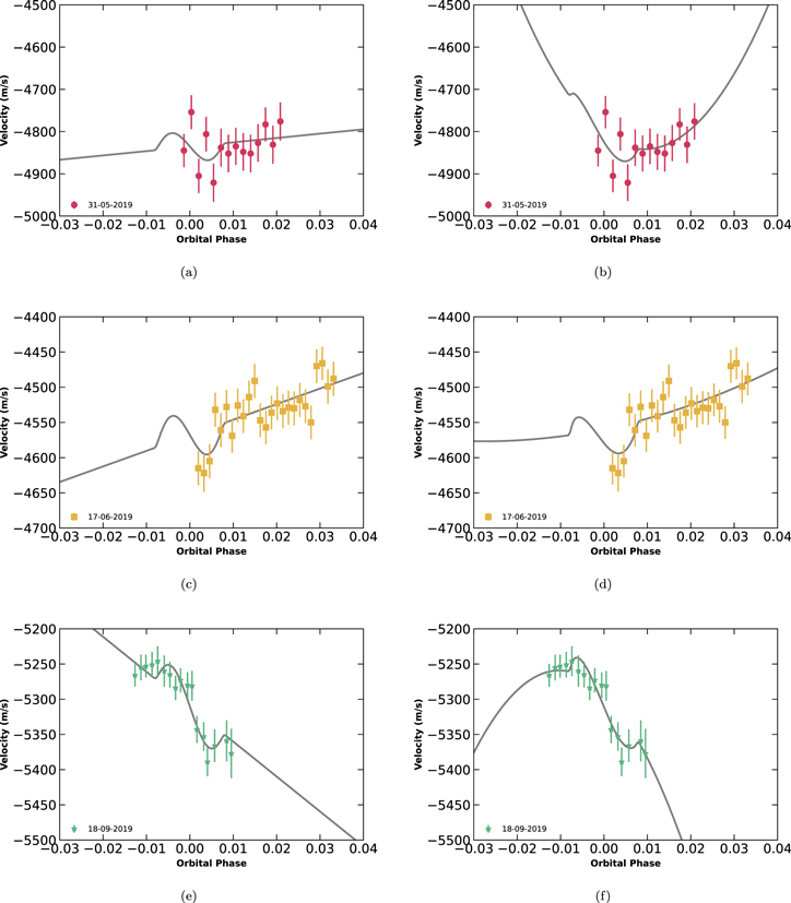
Figure 1. Telescope binned spectroscopic radial velocities of three AU Mic b transits, plotted as a function of orbital phase with the best fitting Rossiter–McLaughlin model + stellar activity model (hybrid linear plotted on the left panels and second order hybrid polynomial plotted on the right panels as the gray line). The transit observation on 2019 May 31 is shown in (a) and (b), 2019 June 17 is shown in (c) and (d), and 2019 September 18 is shown in (e) and (f). The filled red circles, orange squares, and teal stars with error bars are the binned radial velocities obtained in this work on the 2019 May 31, 2019 June 17, and 2019 September 18, respectively.
Download figure:
Standard image High-resolution image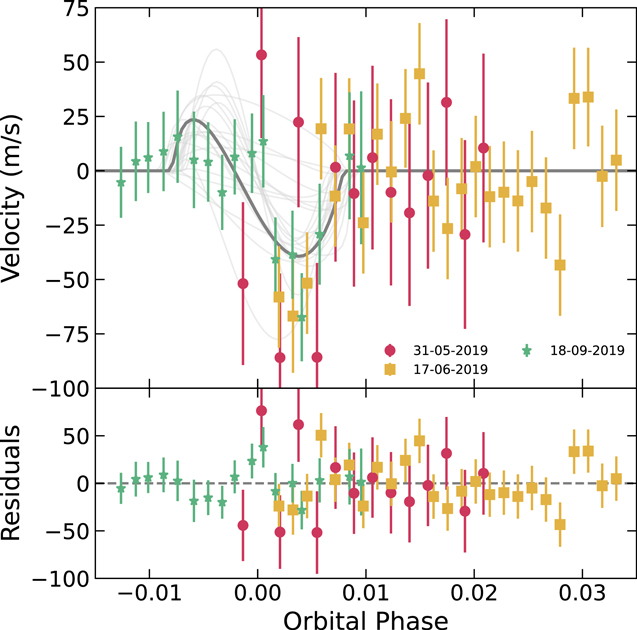
Figure 2. Telescope binned spectroscopic radial velocities of AU Mic, phased to a single transit, plotted as a function of phase with the best-fit median Rossiter–McLaughlin model (solid opaque gray line), 20 Rossiter–McLaughlin models drawn from the posterior (translucent gray lines), and corresponding residuals (from the best-fit model). The second order hybrid polynomial (preferred solution) for each transit observation has been removed from the radial velocities. The filled red circles, orange squares, and teal stars with error bars are the binned radial velocities from the 2019 May 31, 2019 June 17, and 2019 September 18 transit observations, respectively.
Download figure:
Standard image High-resolution image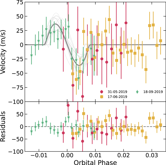
Figure 3. Same as Figure 2, but the stellar activity has been removed using a hybrid linear model.
Download figure:
Standard image High-resolution image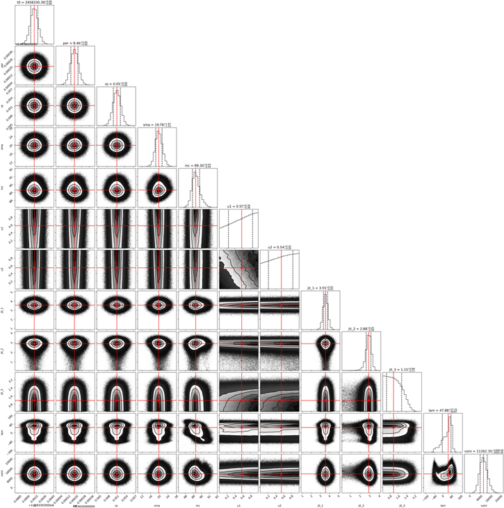
Figure 4. Corner plot of the posteriors using the second order hybrid polynomial activity model.
Download figure:
Standard image High-resolution image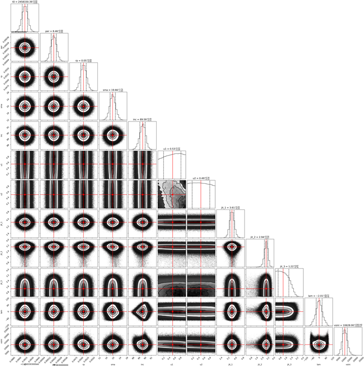
Figure 5. Corner plot of the posteriors using the hybrid linear activity model.
Download figure:
Standard image High-resolution image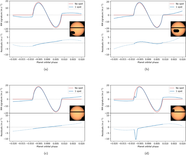
Figure 6. Simulations of AU Mic b’s transit with four different single starspot configurations. In each figure, the top panel shows the Rossiter–McLaughlin signature produced for the planet assumed to be on an aligned orbit (λ = 0°) for an un-spotted stellar surface (red line) and with a single starspot, detrended with a second order polynomial (blue line). The bottom panel shows the residuals between the Rossiter–McLaughlin only model and Rossiter–McLaughlin + starspot model (red curve - blue curve). Shown on the right of each plot are stacked images of the planet (thin horizontal dark streak) and the spot traveling across the surface (thicker dark patch) during the transit event. (a) Starting spot position: θspot = 120° and ϕspot = 300°; (b) starting spot position: θspot = 105° and ϕspot = 330°; (c) starting spot position: θspot = 130° and ϕspot = 70°; and (d) starting spot position: θspot = 70° and ϕspot = 290°. A spot crossing event occurs, resulting in a temporary ∼−10 m s−1 anomaly in the Rossiter–McLaughlin signature.
Download figure:
Standard image High-resolution imageThe lack of full transit coverage for the radial velocities obtained on the 2019 May 31 and 2019 June 17 as well as the lack of sufficient out-of-transit baseline for the full transit observation obtained on the 2019 September 18 renders the complete removal of the stellar activity signal in the radial velocities challenging and a precise measurement of the system‘s sky-projected obliquity impossible. The low-precision obliquity measurement reported here is consistent with the orbit of AU Mic b being well aligned or highly misaligned, but seems to suggest that a retrograde orbit (∣λ∣ ≥ 135°) is unlikely at >3σ.
Our result is consistent with, but less precise than, the low obliquity measured for AU Mic b by other studies submitted in parallel with this paper. These include the Palle et al. (2020) result of  from Rossiter–McLaughlin observations taken with the ESPRESSO spectrograph on the Very Large Telescope array, the Hirano et al. (2020) result of
  from Doppler tomography observations using the IRD spectrograph on the Subaru telescope, and the Martioli et al. (2020) result of
  from Rossiter–McLaughlin observations using the SPIRou spectrograph on the Canada–France–Hawaii Telescope.
3.1. Star Spots
A study by Oshagh et al. (2018) has shown that star spots can lead to variations in the shape of the Rossiter–McLaughlin signal observed in the radial-velocity data, even when no spot crossing events occur during a transit. These variations in the observed signal can lead to biased results for the measured spin–orbit angle of up to ∼42°. With this in mind and given AU Mic‘s extreme youth (∼23 Myr) and chromospheric activity (as observed by TESS), we have investigated the potential effects of star spots on the Rossiter–McLaughlin radial-velocity signal to determine the impact that they may have on the results reported in this work. However, due to the lack of simultaneous photometry obtained during the Minerva-Australis Rossiter–McLaughlin observations as well as the time gap between those observations and when TESS observed AU Mic between 2018 July 25 and August 22 (∼280 days), we have decided not to include a starspot model into the Rossiter–McLaughlin analysis given the high likelihood of the star spots significantly evolving during the time gap.
To highlight the influence of stellar intrinsic variability on the Rossiter–McLaughlin signature, we modeled several different single spot configurations on the stellar surface during a transit of AU Mic b using the spot model of Heitzmann et al., in prep. The star was modeled as a disk of uniform brightness on a pixel grid to which the following elements were added: (i) a quadratic limb-darkening law; (ii) a single spot located at a different colatitude θ and longitude ϕ on the stellar surface for each of the model configurations and with a radius yielding a ∼5% variation in flux over a stellar rotation (as observed by TESS, see Plavchan et al. 2020); and (iii) a transiting planet on an aligned orbit (λ = 0°). The values applied to the stellar and planetary parameters in this model are fixed to the prior values given in Table 3 that were used for the Rossiter–McLaughlin analysis carried out in this work.
Four of the simulations are shown in Figure 6 to highlight the impact of a starspot on the Rossiter–McLaughlin signature. From the trialed starspot configurations, we find that unless the planet directly crosses over a spot, the effect on the resulting radial-velocity Rossiter–Mclaughlin signal (blue line on Figure 6) is small (<5 m s−1 for all spot configurations except for spot crossing events as shown in Figure 6(d)). We also simulated the impact on the Rossiter–McLaughlin effect by including two star spots in the model, each with different locations and sizes (yielding a combined ∼5 % variation in flux over a stellar rotation). We find that the impact on the Rossiter–Mclaughlin signal from the two spot models to be even smaller than the single starspot models.
Given the relatively high uncertainty on each of the radial-velocity measurements obtained withMinerva-Australis (≳20 m s−1), we do not expect star spots to have a significant influence on the recovery of λ from the Rossiter–McLaughlin effect unless AU Mic b happens to cross over a starspot during one of the observed transits.
4. Discussion & Conclusions
We have detected a marginal Rossiter–McLaughlin effect signal of AU Mic b from radial velocity transit observations using the Minerva-Australis telescope array. From these observations, we measured the sky-projected spin–orbit angle between the planet’s orbit and the host star’s spin axis. Due to AU Mic’s extreme youth (∼23 Myr) and significant stellar activity compounded with our observations lacking full transit coverage (for two out of the three transits observed) plus sufficient out-of-transit data, we are unable to precisely measure the planet’s orbital obliquity. We find  for the preferred (and more conservative) hybrid second order polynomial activity model and
  for the hybrid linear activity model.
AU Mic is the youngest exoplanetary system for which a measurement of the spin–orbit alignment has been attempted, and one of only two systems younger than 100 Myr with such measurements as of 2021 June (the other being DS Tuc A; see Benatti et al. 2019; Newton et al. 2019; Montet et al. 2020; Zhou et al. 2020). The vast majority of obliquity measurements to date have been made for hot Jupiters orbiting earlier type and older main-sequence stars (e.g., Winn & Fabrycky 2015). Therefore, AU Mic occupies a unique parameter space and is an excellent laboratory for testing models of planet formation and misalignment.
Given the potential low obliquity measured for AU Mic b in this study as well as confirmed to be of low obliquity by other studies submitted in parallel with this one, it is likely that the planet formed beyond the “ice-line” within the protoplanetary disk around AU Mic and then migrated inwards as a result of its interaction with that disk (e.g., see, Lin et al. 1996; Ida & Lin 2004; Alibert et al. 2005; Wittenmyer et al. 2020) to its current P ∼ 8.5 day orbit (for an opposing view on the in situ formation of Jovian planets; see, e.g., Batygin et al. 2016). Further evidence to support this comes from the fact that AU Mic’s debris disk is observed to be nearly edge on from far-infrared and submillimeter direct imaging (e.g., see Matthews et al. 2015), with a small aspect ratio suggesting a dynamically cold planetesimal population (Schüppler et al. 2015; Daley et al. 2019). Since AU Mic b transits its host star, this strongly suggests that the planet and the disk lie in the same orbital plane. This then increases the likelihood that the stellar inclination is also close to 90° (i.e., the stellar equator is edge on), since it can be expected that protoplanetary disks from which planets form (and the debris disks that mark the remnants of those disks at later epochs) should be orthogonal to the stellar angular momentum vector (though see Ngo et al. 2015 for a mechanism on perturbing a protoplanetary disk out of alignment at the epoch of star and planet formation) as a consequence of the stellar formation process (Toomre 1964; Pollack et al. 1996). Such star-planet-debris disk alignments have been observed for other planetary systems, such as HD 82943 (Kennedy et al. 2013). Therefore, the sky-projected spin–orbit angle likely represents the true orbital obliquity of the system, and the debris disk, planetary orbit, and stellar equator all seem to be well aligned.
It therefore appears unlikely that this planet experienced high-eccentricity driven migration in the past (e.g., planet–planet scattering; Ford & Rasio 2008; or Lidov-Kozai cycling with tidal friction; Fabrycky & Tremaine 2007) given the low orbital obliquity and its youth, but instead sedately migrated inwards via disk-migration mechanisms (Lin et al. 1996). Giant planet formation by the core-accretion model together with type 1 and 2 disk migration to short-period (<10 day) orbits are predicted to operate on timescales of less than 10 Myr (see, e.g., Rice & Armitage 2003; Weidenschilling 2005; Armitage 2013). Since AU Mic is a member of the β Pictoris moving group, the star’s age is well constrained at 23 ± 3 Myr (Mamajek & Bell 2014). Therefore, the planet’s formation by core accretion and subsequent migration via type 1 and 2 disk migration are completely compatible with the observations.
AU Mic now joins the ranks of the few systems that are known to host both planetary and planetesimal components (e.g., Kennedy et al. 2018; Yelverton et al. 2020), making it an even more important analog to the solar system for studying the interplay between planetary and debris components. Furthermore, determining the obliquity distribution of young planetary systems like AU Mic will be crucial in establishing their formation and migration histories, dynamical processes that have a substantial impact on their architectures.
The all-sky transiting exoplanet survey TESS has begun delivering new discoveries of young exoplanets orbiting bright stars that are needed to establish this obliquity distribution, and in the years to come, it is likely that systems such as AU Mic will prove pivotal in placing the formation of our own planetary system in context.
We respectfully acknowledge the traditional custodians of all lands throughout Australia, and recognize their continued cultural and spiritual connection to the land, waterways, cosmos, and community. We pay our deepest respects to all Elders, ancestors, and descendants of the Giabal, Jarowair, and Kambuwal nations, upon whose lands the Minerva-Australis facility at Mt Kent is situated.
Minerva-Australis is supported by Australian Research Council LIEF Grant LE160100001, Discovery Grant DP180100972, Mount Cuba Astronomical Foundation, and institutional partners University of Southern Queensland, UNSW Australia, MIT, Nanjing University, George Mason University, University of Louisville, University of California Riverside, University of Florida, and The University of Texas at Austin.
J.P.M. acknowledges research support by the Ministry of Science and Technology of Taiwan under grants MOST107-2119-M-001-031-MY3, MOST107-2119-M-001-031-MY3, and MOST109-2112-M-001-036-MY3, and Academia Sinica under grant AS-IA-106-M03. M.N.G. acknowledges support from MIT’s Kavli Institute as a Juan Carlos Torres Fellow.
Facility: Minerva-Australis. -