Abstract
We report the first detection of circular polarization in 4.7 GHz excited OH masers in star-forming regions made using full Stokes measurements with the Green Bank 100 m telescope. The Zeeman shift between the two circular components provides a measure of the magnetic field pervading these maser spots. Three different methods are used to determine the shift in velocity between the RCP and LCP components. We find fields with B ∼ 100 mG using archival molecular parameters that have limited precision and uncertain values. Reservations of using 1.7 and 6.0 GHz OH masers to estimate magnetic fields in star-forming regions are discussed.
Original content from this work may be used under the terms of the Creative Commons Attribution 4.0 licence. Any further distribution of this work must maintain attribution to the author(s) and the title of the work, journal citation and DOI.
1. Introduction
Astronomical masers were discovered about 60 yr ago when S. Weinreb et al. (1965) recognized that the narrow lines of “mysterium” suggested by H. Weaver et al. (1965) corresponded to the 1.665 GHz ground state (gs) OH transition. Their narrow widths identified them as maser rather than thermal emission. Soon after this, lines from excited (ex) OH at 4.7 GHz and 6.0 GHz were also discovered by B. Zuckerman et al. (1968) and J. L. Yen et al. (1969), respectively. In all instances, these masers occurred in molecular clouds associated with star-forming regions. Many other species of masers have been detected subsequently in a variety of astronomical environments.
An interesting feature of all the maser lines from 1.7 GHz gsOH and the 6.0 GHz exOH lines in these discovery observations was that they were circularly polarized. These levels are both from the  chain of the OH energy levels, for which it was assumed that this polarization was due to the presence of magnetic fields in the molecular clouds causing Zeeman splitting of the levels of OH. For both species of masers, isolated maser spots of either RCP or LCP emission have been found. These individual spots provide no measure of the magnetic field, only spatially related pairs of spots can be used. In contrast to this, the 4.7 GHz exOH masers were not polarized. However, these masers occur between states in the lowest level of the
  chain, which have a Landé g-factor about 3 orders of magnitude smaller than for the
  levels, so that Zeeman splitting was neither expected nor observed.
Theoretical calculations by H. E. Radford (1961) that were compared with measured Zeeman splitting in OH laboratory experiments showed excellent agreement, giving the Landé gJ values for these levels as gJ = 0.935 and 0.485 for the 1.7 and 6.0 GHz lines respectively. These parameters produce Zeeman splittings of 590 and 236 km s−1 G−1 in the 1.665 and 1.720 GHz gsOH lines, and 79.0 and 56.4 km s−1 G−1 in the 6.031 and 6.035 GHz exOH lines (see Table 1 in R. D. Davies 1974). Note that R. D. Davies (1974) quotes values for the separation between the RCP and LCP components, which is twice the value of the velocity shift due to the Zeeman effect. Based on the calculations of H. E. Radford (1961), a value for the 4.7 GHz lines is given only as ∼10−2 km s−1 G−1. Clearly, the Zeeman splitting of these exOH lines is much smaller than those of lines in the  chain.
Zeeman pairs in gsOH 1.720 GHz masers were definitively identified for the first time by K. Y. Lo et al. (1975), using three station VLBI measurements to show the spatial correspondence of RCP and LCP pairs. Since then 1.7 and 6.0 GHz gs- and exOH masers have regularly been used to determine the strength of magnetic fields in star-forming regions. Results from these observations indicate magnetic fields in the range of 1–10 mG.
The spectra of 18 cm gsOH masers are often complex and have overlapping components in single-dish measurements. Zeeman components can usually only be identified using array measurements showing maps of the maser spots and identifying RCP and LCP components that lie spatially near each other. Often there is less confusion in 6 GHz exOH masers but even so maps of the regions provide a more secure identification of Zeeman pairs than single-dish spectra, although there are problems with this approach as well. Orthogonally polarized pairs of spots with similar velocities are assumed to be at the same line-of-sight (LOS) distance from the observer, but this is not necessarily the case, so some misidentifications can be made. G. C. MacLeod et al. (2023) has recently shown that, given a long enough data set, single-dish spectra can be used to identify Zeeman pairs by tracking RCP and LCP peaks that drift slowly at the same velocity.
Spectra of 4.7 GHz exOH masers are generally far less complicated than the lower energy masers from the  levels, often displaying only a single spot of emission. This makes it possible to study the properties of these masers, such as temporal variations, using single-dish telescopes. Measurements of 4.7 GHz exOH masers have often been observed using circular polarization feeds, but to date no Zeeman splitting has been identified. Linear polarization has been reported in only one 4.765 GHz source thus far; in the 1990s a set of flaring masers in Mon R2 were found to have linear polarization of ∼14% (D. P. Smits et al. 1998) in two separate spots. A later flare from a new spot had the same percentage of linear polarization, leading to the suggestion that the exOH masers were amplifying background radiation that was polarized, rather than being intrinsic to the maser due to magnetic fields.
In this paper we report the first detection of Zeeman pairs in two 4.765 GHz exOH masers, indicating that a magnetic field permeates at least some part of the masing column of gas. In Section 2 we provide brief details of the two sources in which circular polarization has been found, and in Section 3 details of our observations are presented. In Section 4 our results are presented, including a discussion on skewness and how we measured it. In Section 5 our conclusions are presented.
2. Sources
In a survey of 20 sources using the Green Bank Telescope (GBT) and C-band receiver, we found 4.765 GHz masers in eight sources, of which two had circular polarization. These statistics are small so should be treated with caution, but they do suggest that Zeeman splitting in these masers is not necessarily rare. However, it is weak and sensitive observations are required to extract this faint signal from the background noise.
In a search toward IRAS sources identified as star-forming regions by their colors, H2O masers were found in IRAS 05358+3543, also known as G173.482+2.446 (hereafter G173), by J. G. A. Wouterloot et al. (1988). Follow-up observations revealed the presence of weak (Sν < 0.8 Jy) lines of 100% circularly polarized 1.665 GHz gsOH masers at velocities between –10 and –16 km s−1. No 1.667 GHz lines were found at that time, but K. A. Edris et al. (2007) did discover a single line with LCP at v = −10.53 km s−1. At the time of these observations, the 1.665 GHz flux density peaked at 2.82 Jy and covered a range of velocities from –8.5 to −16.5 km s−1. The first detection of 4.765 GHz exOH maser emission in G173 was made by H.-H. Qiao et al. (2022) at velocities of v = −16.83 and –16.31 km s−1 with flux densities of 0.53 and 3.41 Jy respectively.
The other source in which we found Zeeman splitting is G213.705–12.60, which is also known as Mon R2 IRS 3 (hereafter Mon R2). It underwent a major flaring episode at 4.765 GHz in the 1990s (D. P. Smits et al. 1998; D. P. Smits 2003). In addition to regular monitoring using the 26 m telescope of the Hartebeesthoek Radio Astronomy Observatory (HartRAO), a few target-of-opportunity observations of this source were made using MERLIN. An unexpected discovery from those events was that the exOH masers had 14% linear polarization (D. P. Smits et al. 1998). No circular polarization was detected by MERLIN to a level below 1% of the flux density. In 1997 December the maser flux density reached a peak of ∼80 Jy, but only displayed linear polarization. This is the only 4.765 GHz maser that has previously been reported to have polarization.
By the end of 1998 the exOH Mon R2 masers dropped below detectable levels for HartRAO and MERLIN. The 4.765 GHz maser was detected again in 2006 May (V. L. Fish et al. 2006), indicating another flaring episode. The 4.765 GHz masers have been monitored at HartRAO since 2012 and have undergone several flaring episodes during this period. The most recent flaring episodes was detected while observing with the GBT in 2023 and will be reported separately (P. Fallon & D. P. Smits 2025, in preparation), but here we report the first detection of circular polarization in Mon R2, which has appeared during the current flaring episode.
Coordinates and central velocities of the spectra for the two star-forming regions that have observable Stokes V signals are listed in Table 1.
Table 1. Source Name, J(2000) Coordinates, and Central Velocity of the Spectra
| Source | R.A. (J2000) | Decl. (J2000) | Velocity |
|---|---|---|---|
| ID | (hh mm ss.s) | (deg, arcmin, arcsec) | (km s−1) |
| G173.482+2.446 = G173 | 05 39 13.0 | +35 45 51.0 | –16.7 |
| G213.705–12.60 = Mon R2 | 06 07 47.8 | –06 22 56.5 | +10.7 |
Download table as: ASCIITypeset image
3. Observations
All observations reported here were made with the 100 m GBT using the C-band receiver with the Versatile GBT Astronomical Spectrometer (VEGAS) backend in full Stokes mode. Each observing session consisted of a single source together with B0529+075 as a flux density calibrator and 3C138 as a linear polarization calibrator. The Hi-Cal noise diode was used for all except three observations: G173 and Mon R2 on 2023 July 6 and 21 for which the Lo-Cal noise diode was used. Subsequent observations were made using the Hi-Cal noise diode with an expectation that this would result in improved measurement stability. However, the ongoing observations have not indicated improvements in accuracy or stability using the Hi-Cal noise diode. The setup and calibrators took up about 50 minutes, giving on-source observations of up to 1.5 hr. All scans were checked individually for RF noise, and, when present, those scans were discarded, so most sessions ended up being shorter than this. Programs to analyze position- and frequency-switching observations to obtain full Stokes polarization were developed as part of project AGBT20B–424 and are described in GBT Memo 306 (P. Fallon 2022). Calibrators were observed using position-switching by offsetting from the target source by  , while spectra were obtained using frequency-switching of −2.9 MHz (approximately the GBT default value of –0.25*bandwidth) to maximize the on-source time.
The VEGAS backend contains eight bands, each of which is operated in mode 15, providing a bandwidth of 11.72 MHz over 32 768 channels, corresponding to a frequency resolution of 357.7 Hz. This gives a velocity resolution of 0.0225 km s−1 and a velocity range of ∼−300 to +300 km s−1 at 4.765 GHz. The rest frequency used for the F = 1 → 0 transition in the  level of exOH was 4.765 562 GHz (J. L. Destombes et al. 1977). Two other channels were used to look at the 4.660 and 4.750 GHz lines but no maser detections were found above a 1σ level of the rms noise listed in Table 2 for each observation at these frequencies.
Table 2. Details of Observations and Gaussian Fits to G173 (G) and Mon R2 (1–16)
| # | Date | Obs. | Gaussian Fit to Thermal Comp | Single Gaussian Fit to Stokes I | 2 Gaussian | |||||
|---|---|---|---|---|---|---|---|---|---|---|
| Observed | Time | rms | Flux Density | Velocity | FWHM | Flux Density | Velocity | FWHM | Fit to I | |
| (yyyy mmm dd) | (minutes) | (mJy) | (Jy) | (km s−1) | (km s−1) | (Jy) | (km s−1) | (km s−1) | Skewness | |
| G | 2023 Apr 23 | 68 | 16 | 0.600(3) | –16.6697(7) | 0.2645(17) | 0.17 | |||
| 1 | 2023 Jul 06 | 28 | 92 | 0.099(10) | 11.14(8) | 1.62(16) | 12.77(2) | 10.7216(2) | 0.2999(5) | −0.001 |
| 2 | 2023 Jul 21 | 50 | 66 | 0.103(7) | 11.11(5) | 1.67(10) | 11.38(1) | 10.7201(2) | 0.2993(4) | 0.015 |
| 3 | 2023 Dec 23 | 70 | 59 | 0.087(6) | 11.19(6) | 1.57(10) | 16.27(3) | 10.7017(2) | 0.2854(5) | 0.146 |
| 4 | 2024 Jan 27 | 90 | 48 | 0.079(5) | 11.24(6) | 1.73(11) | 19.11(3) | 10.6986(2) | 0.2822(5) | 0.166 |
| 5 | 2024 Feb 20 | 54 | 76 | 0.096(9) | 11.13(7) | 1.68(13) | 20.72(3) | 10.6973(2) | 0.2797(5) | 0.180 |
| 6 | 2024 Apr 03 | 70 | 64 | 0.082(7) | 11.08(6) | 1.82(13) | 21.10(3) | 10.6943(2) | 0.2764(5) | 0.194 |
| 7 | 2024 Apr 28 | 48 | 70 | 0.083(7) | 11.34(8) | 1.50(15) | 25.49(4) | 10.6906(2) | 0.2744(5) | 0.216 |
| 8 | 2024 May 22 | 68 | 59 | 0.084(6) | 11.10(6) | 1.82(12) | 21.78(4) | 10.6886(2) | 0.2715(5) | 0.238 |
| 9 | 2024 Aug 18 | 42 | 99 | 0.098(12) | 11.11(9) | 1.72(17) | 21.85(4) | 10.6863(3) | 0.2628(6) | 0.276 |
| 10 | 2024 Oct 05 | 48 | 92 | 0.074(8) | 11.25(11) | 2.11(21) | 18.85(4) | 10.6914(3) | 0.2619(6) | 0.273 |
| 11 | 2024 Nov 05 | 38 | 76 | 0.107(10) | 11.08(6) | 1.61(11) | 17.08(3) | 10.6950(2) | 0.2612(6) | 0.248 |
| 12 | 2025 Jan 27 | 66 | 58 | 0.086(6) | 11.11(5) | 1.70(11) | 15.17(2) | 10.7073(2) | 0.2663(5) | 0.203 |
| 13 | 2025 Feb 24 | 38 | 91 | 0.115(13) | 11.00(6) | 1.40(12) | 17.12(3) | 10.7121(2) | 0.2679(5) | 0.182 |
| 14 | 2025 Mar 19 | 70 | 57 | 0.078(6) | 11.06(6) | 1.98(13) | 20.28(3) | 10.7149(2) | 0.2712(5) | 0.173 |
| 15 | 2025 Apr 11 | 64 | 78 | 0.083(9) | 11.21(8) | 1.52(15) | 22.98(3) | 10.7171(2) | 0.2747(5) | 0.148 |
| 16 | 2025 May 02 | 60 | 61 | 0.100(7) | 11.05(5) | 1.68(10) | 26.21(4) | 10.7187(2) | 0.2773(5) | 0.145 |
Note. The first column labels the observations to identify the entry in other tables. There is no discernible thermal component in the G173 spectrum.
Download table as: ASCIITypeset image
We followed a standard procedure to analyze the spectra, which were recorded every 2 minutes. Each spectrum was first shifted and folded and then calibrated using the standard value. A baseline was fitted to the velocity range for G173 between [−32, −22] and [−11, −1] km s−1 and for Mon R2 over [−18, +2] and [+18, +30] km s−1, using a third-order polynomial; this broad exclusion range for Mon R2 ensured that the thermal component was not included in the baseline subtraction process. Our Mueller matrix was then applied to the individual spectra, which were then added together to produce the on-sky I, Q, U, V measurements.
We make use of the Mueller matrix for the C-band system as described by P. Fallon et al. (2023), with some modifications. First, the Mueller matrix component M4,4 is set to –1 rather than +1 to give the polarization orientation in agreement with other instruments. Because the circular polarization of calibrators 3C138 and 3C286 is taken to be zero, the orientation of Stokes V was not set during the Mueller matrix calibration. The –1 setting aligns with the –1 of the M2,2 and M3,3 components, and the GBT receiver’s orientation. Due to instability in both the intensity and polarization between the single position-switched scans of 3C138, in particular in the latter part of 2024 and during 2025, several 3C138 observations were excluded and an average Mueller matrix value was used initially for all observations. Further checks on the Mueller matrix values were made with observations of 3C286 in 2025 April and May. A further small Mueller matrix refinement was made when fitting dI/dv to Stokes V (Method 3 in Section 4.5). The fitting process highlights the need for Mueller matrix corrections, described by T. H. Troland & C. Heiles (1982) and M. Elitzur (1998), which is due to leakage of Stokes I into Stokes V. Once this Mueller matrix adjustment was implemented, all analyses were rerun.
All Gaussians fitted to our data made use of the least squares fitting routine in GBTIDL.
4. Results
4.1. G173.482+2.446 = G173
Only one observation was made of this source, the date and duration of which are presented in Table 2 labeled G. Our 4.765 GHz I spectrum is shown in black in Figure 1(a). Parameters of a Gaussian profile fitted to the Stokes I component, shown in red on the plot, are listed in Table 2. This maser, with a flux density of only Sν = 0.6 Jy, is weak and, hence, has a poor signal-to-noise ratio (SNR). Our measured flux densities and velocities of our fitted Gaussians are different from those of 0.53 and 3.41 Jy at v = −16.83 and –16.31 km s−1 reported by H.-H. Qiao et al. (2022), so there is clearly some variability in the source between the two sets of observations.
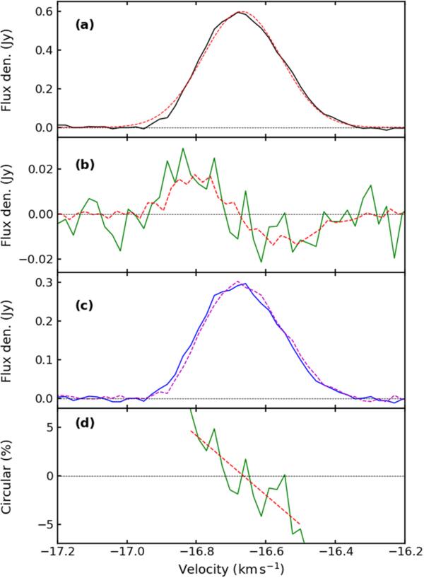
Figure 1. Spectra of (a) Stokes I, (b) Stokes V, (c) RCP and LCP, and (d) V / I for the 4.765 GHz exOH maser in G173.
Download figure:
Standard image High-resolution imageNo linear polarization was found above the noise level, but we did find circular polarization at a level of 5% as can be seen from the green line in Figure 1(b), which is noisy due to the low SNR for this data. This V spectrum shows the characteristic sine-wave shape expected when the velocity shift between RCP and LCP Gaussian profiles is small, as first pointed out by J. A. Galt et al. (1960; see their Figure 1). The red line is a plot of scaled dI/dv determined from the Stokes I profile in Figure 1(a) and is a good fit to the green line. The green line in Figure 1(c) is a plot of Stokes V/I as a percentage, and the red line is a straight-line fit to this data over the width of the emission.
The sine-shaped curve of the V spectrum and the straight-line fit to the V/I plot are consistent with (but not exclusive to) a single spot of circularly polarized emission (see Appendix A). However, the sine-shaped curve lacks the symmetry of a pure theoretical treatment. This asymmetry will be addressed later when we discuss the skewness parameter presented in Table 2.
The circular components of the maser signal were determined using RCP = (I + V)/2 and LCP = (I − V)/2. The parameters of single Gaussians fitted to these profiles are listed in Table 3 in the top row labeled G. Following standard practice, the full width at half maximum (FWHM) of the maser profiles are listed rather than the standard deviation σ of the Gaussians. They are related by FWHM 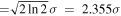 .
.
Table 3. Gaussian Parameters of RCP and LCP Components for G173 (G) and Mon R2 (1–16)
| # | Single Gaussian Fit to RCP | 2 Gaussian | Single Gaussian Fit to LCP | 2 Gaussian | Amplitude | ||||
|---|---|---|---|---|---|---|---|---|---|
| Flux Density | Velocity | FWHM | Fit to RCP | Flux Density | Velocity | FWHM | Fit to LCP | Ratio | |
| (Jy) | (km s−1) | (km s−1) | Skewness | (Jy) | (km s−1) | (km s−1) | Skewness | f | |
| G | 0.299(2) | –16.6743(9) | 0.267(2) | 0.16 | 0.302(2) | –16.6653(9) | 0.262(2) | 0.19 | 1.009(11) |
| 1 | 6.39(1) | 10.7243(3) | 0.2998(6) | −0.001 | 6.39(1) | 10.7189(2) | 0.2999(5) | 0.000 | 1.000(2) |
| 2 | 5.69(1) | 10.7227(2) | 0.2992(5) | 0.015 | 5.69(1) | 10.7174(2) | 0.2992(4) | 0.013 | 1.000(2) |
| 3 | 8.14(1) | 10.7043(2) | 0.2854(5) | 0.144 | 8.14(1) | 10.6991(2) | 0.2854(5) | 0.149 | 1.000(2) |
| 4 | 9.56(1) | 10.7013(2) | 0.2819(5) | 0.169 | 9.55(1) | 10.6959(2) | 0.2822(5) | 0.164 | 0.999(2) |
| 5 | 10.35(2) | 10.6998(2) | 0.2802(5) | 0.176 | 10.37(2) | 10.6948(2) | 0.2791(5) | 0.185 | 1.002(2) |
| 6 | 10.56(2) | 10.6970(2) | 0.2762(5) | 0.190 | 10.55(2) | 10.6916(2) | 0.2764(5) | 0.199 | 1.000(2) |
| 7 | 12.75(2) | 10.6932(2) | 0.2742(5) | 0.203 | 12.74(2) | 10.6879(2) | 0.2744(5) | 0.230 | 1.000(2) |
| 8 | 10.89(2) | 10.6913(2) | 0.2717(5) | 0.231 | 10.90(2) | 10.6860(2) | 0.2712(5) | 0.243 | 1.001(2) |
| 9 | 10.93(2) | 10.6891(3) | 0.2627(6) | 0.267 | 10.93(3) | 10.6835(3) | 0.2628(7) | 0.281 | 1.000(3) |
| 10 | 9.43(2) | 10.6944(3) | 0.2619(6) | 0.266 | 9.43(2) | 10.6885(3) | 0.2617(6) | 0.275 | 1.000(3) |
| 11 | 8.55(2) | 10.6977(3) | 0.2607(6) | 0.241 | 8.54(2) | 10.6922(3) | 0.2615(6) | 0.254 | 0.999(3) |
| 12 | 7.59(1) | 10.7102(2) | 0.2660(5) | 0.210 | 7.58(1) | 10.7044(2) | 0.2664(5) | 0.193 | 0.999(2) |
| 13 | 8.56(2) | 10.7147(2) | 0.2678(6) | 0.183 | 8.56(2) | 10.7095(3) | 0.2679(6) | 0.182 | 1.000(3) |
| 14 | 10.14(2) | 10.7179(2) | 0.2711(5) | 0.170 | 10.15(2) | 10.7119(2) | 0.2710(5) | 0.172 | 1.000(2) |
| 15 | 11.49(2) | 10.7200(2) | 0.2745(5) | 0.149 | 11.49(2) | 10.7142(2) | 0.2747(5) | 0.147 | 1.000(2) |
| 16 | 13.11(2) | 10.7215(2) | 0.2770(5) | 0.146 | 13.10(2) | 10.7159(2) | 0.2774(5) | 0.145 | 0.999(2) |
Download table as: ASCIITypeset image
4.2. G213.705–12.60 = Mon R2
A new feature in the I spectra of the 4.765 GHz exOH emission in Mon R2 is the presence of a broad thermal component. This profile has been observed in all our spectra taken with the GBT (including one where there was no significant maser emission). In Figure 2 this thermal component is shown on 2021 November 27 before the recent flaring episode began, and on 2024 January 27 when the maser had a flux density Sν 19.11 Jy. This signal is too weak to be identified in the HartRAO spectra, and because thermal emission usually occurs over a large area, it would have been resolved out by MERLIN observations. Hence, if this thermal component has been present since the 1990s, it would not have been noticed in previous observations. Because the Q, U, and V spectra are the difference between two orthogonal components, the thermal component, which is assumed to be unpolarized, is automatically absent.
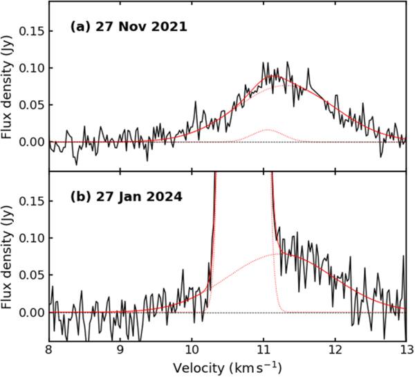
Figure 2. The thermal emission in the 4.765 GHz Mon R2 spectrum on (a) 2021 November 27 and (b) 2024 January 27. The black line is the observed data, the dotted red lines are fits to the idnvidual Gaussians, and the solid red line is a sum of the individual components.
Download figure:
Standard image High-resolution imageWhen the maser started flaring again in mid 2023, the thermal profile was still present and had to be subtracted from the spectra to determine the pure maser emission. To achieve this, the I spectrum was fitted with two or three Gaussians: one for the thermal profile and the other one or two to model the maser emission. For all observations except that on 2023 July 6, a single Gaussian fitted to the maser emission left large residuals, but when two Gaussians were fitted the residuals consisted only of noise. This fitting procedure gave the parameters for the thermal Gaussian profile, which could then be subtracted from the I spectra to leave the maser components.
In Table 2 the observation dates of Mon R2 are listed together with the time spent on-source, and the ensuing rms noise in our spectra. Gaussian parameters fitted to the thermal and Stokes I components for each session are also listed, together with the skewness of the I profile, which will be discussed in more detail in Section 4.4.
The thermal emission variability between the observations is larger than the uncertainties in the fitted Gaussian parameters. This could be due to extracting a weak signal from the maser signal, which is 2 orders of magnitude larger than the thermal flux density. An observation made on 2021 November 27 had almost no maser emission so the spectrum was dominated by the thermal component. A Gaussian profile fitted to this spectrum had a flux density Sν = 76(6)mJy, a central velocity v = 11.32(4) km s−1, and an FWHM Δv = 1.60(8) km s−1, where the figures in parentheses are the uncertainties of the least significant figures. Adding the thermal components of all our 18 observations of Mon R2 together and then fitting a Gaussian gives parameters of peak flux density Sν = 87(1) mJy, velocity of peak v = 11.143(12) km s−1, and FWHM Δv = 1.71(3) km s−1. This is noticeably different from the values from 2021 November 27, which could indicate that the maser has an influence on the thermal component. This will require further investigation.
Plots of the Stokes I, Stokes V, RCP and LCP, and V/I for two epochs are shown in Figure 3. The black I component is the data, fitted with a single Gaussian in red. The green V profile displays the sine-wave shape expected for the difference between two closely spaced Gaussians and is fitted well by the derived scaled red dI/dv curve. In the 2023 July 6 spectrum, the V shape is reasonably symmetrical while in all other Mon R2 (and G173) observations reported here, there is an asymmetry between the positive and negative sections of the V profile. In the bottom plot the green V/I data is fitted with a red straight line.
Figure 3. Spectra of (a) and (e) Stokes I, (b) and (f) Stokes V, (c) and (g) RCP and LCP, and (d) and (h) V/I of the 4.765 GHz exOH maser in Mon R2 on 2023 July 6 and 2024 January 27 .
Download figure:
Standard image High-resolution imageThe circular components of the maser signal were determined using RCP = (I + V)/2 and LCP = (I − V)/2. The parameters of single Gaussian profile fitted to these data are presented in Table 3. The velocity separation 2δ between the RCP and LCP components is small; δ measured from the Gaussian fits is listed in Table 4 together with values determined by two other methods, which are described in Section 4.5.
Table 4. Velocity Shift δ for G173 (G) and Mon R2 (1–16) Using Three Different Methods as Discussed in the Text
| # | δ (10−3 km s−1) | BLOS | ||
|---|---|---|---|---|
| Method 1 | Method 2 | Method 3 | (mG) | |
| G | –4.5(18) | –3.9(7) | –4.3(5) | –137(15) |
| 1 | 2.71(17) | 2.54(16) | 2.68(12) | 85(4) |
| 2 | 2.69(13) | 2.68(9) | 2.68(9) | 85(3) |
| 3 | 2.60(14) | 2.69(11) | 2.59(5) | 82.2(17) |
| 4 | 2.71(14) | 2.76(8) | 2.70(4) | 85.9(11) |
| 5 | 2.49(15) | 2.57(7) | 2.46(6) | 78.0(19) |
| 6 | 2.70(15) | 2.85(9) | 2.68(5) | 85.3(16) |
| 7 | 2.69(15) | 2.92(7) | 2.66(5) | 84.7(15) |
| 8 | 2.65(16) | 2.60(8) | 2.62(4) | 83.3(13) |
| 9 | 2.76(20) | 2.88(9) | 2.74(7) | 87(2) |
| 10 | 2.95(18) | 3.02(10) | 2.92(6) | 92.9(19) |
| 11 | 2.73(18) | 3.00(11) | 2.73(7) | 87(2) |
| 12 | 2.91(16) | 2.91(10) | 2.89(5) | 92.0(15) |
| 13 | 2.60(17) | 2.51(14) | 2.58(6) | 82.2(19) |
| 14 | 2.97(15) | 3.01(9) | 2.94(5) | 93.6(17) |
| 15 | 2.92(15) | 3.06(11) | 2.92(6) | 92.7(17) |
| 16 | 2.83(14) | 2.89(11) | 2.83(4) | 89.8(11) |
Note. The magnetic field BLOS is calculated from Method 3 using a conversion factor 0.0315 km s−1 G−1.
Download table as: ASCIITypeset image
4.3. Temporal Changes in the Mon R2 Line Profile
The evolution of the Mon R2 flaring can be traced using the data from Tables 2 and 3. The peak flux density I, the peak velocity μ, and the FWHM are plotted in Figures 4(a), (b), and (c), respectively, together with the values for the RCP and LCP components. The amplitudes of the circular components are similar and follow the behavior of the Stokes I flux density. The peak velocities μ of the three components all vary synchronously with a fairly constant separation between each of them. The FWHM of the single Gaussian profiles show that all three components vary synchronously. This gives us confidence that the fitted functions are reliable measures of the line profiles.
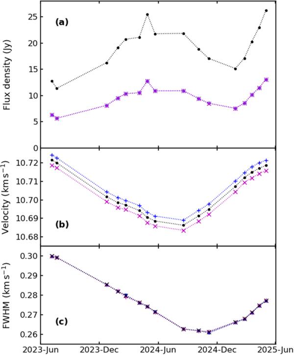
Figure 4. Time variation of (a) the peak flux density, (b) peak velocity μ, and (c) FWHM for the Mon R2 Stokes I, RCP, and LCP maser profiles. The error bars are included, but are smaller than the markers.
Download figure:
Standard image High-resolution imageThe variations in the flux density are an intrinsic property of the maser, whereas the variations in the peak velocity μ and the FWHM appear to be related to the skewness. Long-term monitoring of masers shows that the central velocity may drift slowly with time (G. C. MacLeod et al. 2023), but not usually over the short time periods of our data. The width of maser profiles can vary if they are made up of multiple spots of emission that cannot be resolved in space or velocity, but the sine-wave shape of the V curves is consistent with a single spot of maser emission, which should remain constant. A more likely explanation for the temporal changes in μ and FWHM is that they are due to the influence of the skewness, which affects the values of these two fitted Gaussian parameters. Skewness is discussed in the next section.
4.4. Maser Line Profile Skewness
The f parameter listed in Table 3 is a measure of the difference in amplitude between the RCP and LCP profiles. Because the f values all have values close to unity, the asymmetry between the positive and negative portions of the Stokes V sine curve cannot be due to amplitude differences between the circular components. An unexpected observation from this study is that the Stokes I, RCP, and LCP maser line profiles are distorted Gaussians. The models of interstellar H2O masers developed by W. D. Watson et al. (2002) examined the second-order deviation of Gaussian symmetry known as kurtosis, but did not look at the third-order asymmetry known as skewness. Unsaturated methanol lines have been found to display kurtosis (L. Moscadelli et al. 2003). Both the G173 and Mon R2 sources have a single maser line profile and show a measure of skewness that is evident when trying to fit the spectra with a single Gaussian.
Skewness in Gaussian profiles of maser lines has been considered previously (W. H. T. Vlemmings & H. J. van Langevelde 2005); however, for comparison of masers with different intensity and FWHM, it is important to use a normalized skewness formula. The asymmetry of the maser lines was measured using Fisher’s moment coefficient of skewness (D. N. Joanes & C. A. Gill 1998), given by
where  is the velocity distribution mean and σs is its standard deviation. The spectrum data are represented by velocity vi and intensity Si in each channel. Because noise on either side of the maser line contributes to the value of skewness, the calculation is sensitive to
  and the velocity range used. After testing, a range of
  was used. This is sufficient to include all the skewness of the distribution, while minimizing the noise on either side of the maser line. The center velocity μ and standard deviation σ of a Gaussian fit to the maser line are not the same as
  and σs of the skewed distribution. Hence, an iterative process was used to determine values for
  and σs, using the Gaussian fit parameters as starting values.
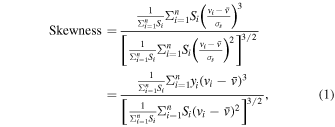
The skewness of the Mon R2 Stokes I, RCP, and LCP Gaussian profiles determined using Equation (1) are plotted in Figure 5(a). Noise in the data, in particular at the tails of the distribution, affects the skewness calculation. This introduces deviations in the calculated skewness, which produces erratic behavior, as can be seen in the plot. Overall, the skewness in all three components follows a similar pattern, showing a slow rise followed by a fall.
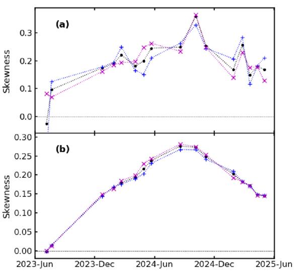
Figure 5. Mon R2 maser line profile skewness generated from (a) the spectral data and (b) a two Gaussian fit to the skewed profiles.
Download figure:
Standard image High-resolution imageTo try and improve the calculations, an alternative method of measuring skewness was tested. In all cases, we found we could fit the skewed profiles with two Gaussians, leaving residuals no larger than the noise. It is beyond the scope of this paper to determine if the two Gaussian fit is a general feature of a skewed Gaussian profile, or if we were just fortunate to be able to restrict the fits to only two components. These two Gaussians were added together to produce a profile that is not affected by the noise associated with the observed data. This summed profile was then analyzed using Equation (1). The skewness calculated using the two Gaussian model is shown in Figure 5(b). Comparison with Figure 5(a) shows a much smoother change in skewness.
The skewness plotted in Figure 5(b) has an inverse behavior to that of the center velocity μ and FWHM shown in Figures 4(b) and (c), suggesting that the changes in these parameters are related to variations in the skewness of the profile. Using our two Gaussian model, the peak velocity of the combined spectra was calculated, and it also underwent shifts matching the behavior of the single Gaussian fits. Therefore, it appears that the skewness is affecting the physical conditions in the column of masing gas. It is noteworthy that the skewness is not related to the intensity of the maser, but it does affect the peak velocity and FWHM. This is clearly an area that needs to be investigated further.
Our analysis suggests several reasons why our data represent skewed profiles as opposed to two overlapping maser lines.
Modeling Stokes V using each profile from the two Gaussian model and then adding them together produces V spectra that do not match our observed data.
The smooth change in skewness seen in Mon R2 (see Figure 5(b)), and the corresponding changes in the maser velocity and FWHM, appear to be related. In contrast, heights for the two fitted Gaussians display a less coherent variation over time.
Finally, e-MERLIN imaging of the Mon R2 maser on 2024 October 14 produced only one spot of emission at its resolution of 40 mas. Assuming a distance of 830 pc to Mon R2, this corresponds to ∼33 au. This does not rule out the possibility of two unresolved maser spots, but a single spot is consistent with our results.
4.5. Determination of Velocity between Circular Components
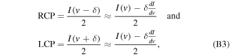
The separation in velocity between the circular components is equal to 2δ where ±δ is the shift in velocity due to the Zeeman effect on the RCP and LCP components from the zero B field position. The value of δ has been determined using three different methods, not all of which are independent. However, the different methods do provide a consistency check on the various values.
Method 1. The RCP and LCP profiles have been fitted with single Gaussians to determine the amplitude A, central velocity μ, and FWHM of the lines. Our velocity spectral resolution of 0.0225 km s−1 facilitated using about 30 channels to fit the line profiles, thereby producing velocity uncertainties lower than the resolution of the spectra.
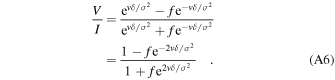
Method 2. In Appendix A it is shown that if the RCP and LCP profiles are formed from single spots of emission with Gaussian shapes, then, provided δ ≪ σ, V/I is a straight line with a slope m = δ/σ2 (Equation (A8)). By fitting a straight line to the observed V/I plot, and using σ from the Gaussian fitting procedure, a value for δ can be determined. Because this method relies on results from the Gaussian fitting procedure it is not an independent method. Unfortunately, skewness has an influence on the straight line and hence the method’s accuracy, which we have not found a way to cater for.
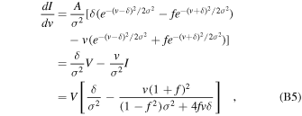
Method 3. When the separation between RCP and LCP is small, the derivative of the Stokes I spectrum with respect to v is proportional to the Stokes V spectrum. Specifically for Gaussians of equal amplitude dI/v = −V/δ, as shown in Appendix B. As seen in Figures 1 and 3, the scaled dI/dv fits the V spectrum remarkably well. This approach has been used previously to determine magnetic field strengths of Zeeman split lines (T. H. Troland & C. Heiles 1982; I. Kazes & R. M. Crutcher 1986; R. M. Crutcher et al. 1993; F. Yusef-Zadeh et al. 1996).
The values of δ determined using the above three methods produce similar results as seen in Table 4 for G173 (G) and Mon R2 (1–16) and plotted in Figure 6. Method 1 can be applied under all circumstances, whereas Methods 2 and 3 are only applicable if δ ≪ σ, which is the situation for these measurements. Method 1 and Method 3 have similar values but the uncertainties for Method 1 are larger than for Method 3. Because the profiles are skewed Gaussians, the straight-line relationship for V/I is affected and produces values that differ from the other two methods, but not by much. Method 3 relies on fitting only one parameter, thereby producing the smallest uncertainties. The strength of the LOS magnetic field BLOS has been calculated from the values of Method 3.
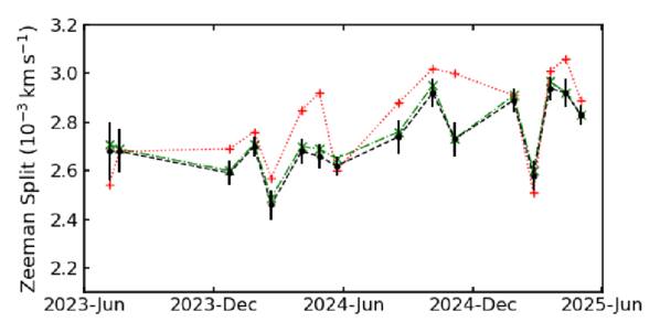
Figure 6. Temporal variations of the velocity shifts due to the Zeeman effect in Mon R2. Method 1 is given by green × and a dashed–dotted line, Method 2 is given by red + and a dotted line, and Method 3 is given by black • and a dashed line. The error bars are from Method 3 in Table 4.
Download figure:
Standard image High-resolution imageIn Table 1 of R. D. Davies (1974), an approximate value for the conversion factor ν/B ∼ 10−3 MHz G−1 for the separation between the RCP and LCP components is given. For our determinations of the magnetic field strength B, which are based on δ rather than 2δ, we set ν/B = 5 × 10⁻⁴, which gives a value v/B = 3.15 × 10⁻² km s−1 G−1 with which to calculate B from our velocity measurements. This factor is still uncertain and could be higher or lower than this, but it is easy to modify our values if, or when, a more reliable value becomes available. Based on this conversion factor the Landé factor for the  J = 1/2 level is gJ = 3.5 × 10⁻⁴, which is smaller than the uncertainties in the current values for gJ in the gs and first excited state of OH.
The observed maser circular polarization results from the portion of the magnetic field B along the observer’s LOS, which for B at an angle θ to the LOS becomes  . The value of θ cannot be determined from the circular polarization measurements alone, the linear component is needed for this. The negative BLOS value for G173 and the positive value for Mon R2 indicate one field pointing away from the observer and the other towards the observer, depending on the convention adopted (see T. Robishaw & C. Heiles 2021; their Section 6.3).
As shown in Figure 6 and Table 4, the velocity shift values change over time, with uncertainties smaller than the variations. We believe these changes are real and are related to variations seen in the maser’s linear polarization (P. Fallon & D. Smits 2024). These polarization changes and the mechanism causing them will be presented separately (P. Fallon & D. P. Smits 2025, in preparation).
There are no 6.0 GHz exOH maser observations toward either of these sources with which to compare magnetic field measurements, but there are some gsOH surveys that have been done, as well as some methanol observations.
The VLA survey of A. L. Argon et al. (2000) found four spots of 1665 gsOH masers toward G173, all with LCP only. The velocities of these spots differ by 4–7 km s−1 from the 4.765 GHz maser so they are probably in a separate position. K. A. Edris et al. (2007) found one spot each of 1.665 and 1.667 GHz lines at LCP only at velocities of v = −10.88 and −10.53 km s−1, which are different from those of the earlier VLA discoveries. Full Stokes observations were made by M. Szymczak & E. Gérard (2009) who found 1.665 and 1.667 GHz masers with both RCP and LCP, but the LCP components were much stronger than the RCP spots, so that Stokes V was nearly 100% LCP. No Zeeman pairs were identified. These spots did not have a high degree of linear polarization. VLA observations made by O. S. Bayandina et al. (2021) found five spots of 1.665 GHz RCP and two of LCP but no obvious Zeeman pairs and the velocities were different from our 4.765 GHz maser. At 1.667 GHz there was one spot each of RCP and LCP but they were at different positions so not a Zeeman pair. The velocities of the gsOH lines have varied in each of the above observations, indicating that this is a source that is undergoing changes. The isolated RCP and LCP spots are consistent with a magnetic field that is stronger than 10 mG, allowing only one mode to grow.
Observations of Zeeman splitting in the methanol 6.7 GHz line were made using the Effelsberg 100 m telescope by W. H. T. Vlemmings (2008). The nonparamagnetic methanol molecule has a small Landé g-factor, producing a separation of 0.049 km s−1 G−1. A magnetic field of B = 19(2) mG was measured at a velocity around v = −13 km s−1. This is about 7 times smaller than our estimate but it is also at a different velocity and in the opposite direction from the magnetic field we measured.
Mon R2 was found to have 1.665 and 1.667 GHz maser spots in both RCP and LCP in the VLA survey of A. L. Argon et al. (2000), but none of these spots manifested as Zeeman pairs. The M. Szymczak & E. Gérard (2009) full Stokes survey found RCP and LCP spots in 1.665 and 1.667 GHz, dominated by the RCP components. The 1.667 GHz Stokes V component has a sine-wave shape, which could indicate Zeeman splitting but the positions of the spots were not determined with enough resolution to locate them at the same position. The peaks of the sine wave are separated by ∼1 km s−1 so if they were a Zeeman pair the magnetic field would be <10 mG and the maser spot velocities are slightly different from that of the 4.765 GHz maser, so probably not in the same region.
There are methanol 6.7 GHz masers in the Mon R2 region, but they are variable and at slightly different velocities from the 4.7 GHz exOH maser. G. Surcis et al. (2015) detected some weak linear polarization (Pl < 5%), and one spot with circular polarization of 0.6%. The magnetic field associated with this spot was very weak.
Conventional wisdom posits that magnetic fields in star-forming regions lie in the range of 1–10 mG. These measurements have been made predominantly using the Zeeman splitting of 1.7 and 6.0 GHz masers, which are sensitive to fields in this range. The problem with this method is that it is not sensitive to fields much stronger than 10 mG. As the field strength grows, so too does the separation between the RCP and LCP components. If this separation becomes large enough, velocity coherence along the length of the maser will only occur in one component, the other one will not be amplified. In array maps of star-forming regions, isolated RCP and LCP spots are seen, but these cannot be used to determine magnetic field strengths. This is a limitation of the currently used OH masers to measure magnetic fields: they can only measure fields within a limited range of strength, above that only one component appears as a maser, and so the field strength cannot be determined. Stronger fields could exist, but a different tool is needed to measure them. Zeeman splitting of 4.7 GHz exOH masers is a tool that can measure stronger fields than those of the gs and 6.0 GHz exOH maser lines.
The 13.441 GHz F = 4 → 4 transition of the  , J = 7/2 state of OH has also been used by J. L. Caswell (2004) to measure magnetic fields in star-forming regions. These masers are rare, which suggests they require very specific conditions for their existence. The Landé g-factor for this transition is smaller than for the 1.7 and 6.0 GHz OH masers, producing a velocity separation of 0.018 km s−1 mG−1. The maximum magnetic field measured by J. L. Caswell (2004) was 10.7 mG, with no single polarity spots being found, but given their delicate nature these masers might also not support large Zeeman shifts. It might be worth searching again for these and other excited OH masers to see what size fields they occur in.
5. Conclusion
The first examples of Zeeman splitting in 4.7 GHz exOH masers are presented here. We have determined reliable values for the velocity shifts due to the Zeeman effect, but because the value of the Landé g-factor is poorly known, we cannot determine an accurate value for the magnetic field. Perhaps these observations will spur someone to look at this problem in more detail and provide a better value. Because we have used the historical estimate of the conversion factor, the strength of magnetic fields associated with these Zeeman shifts are larger than have been measured previously in star-forming regions. As an example, if the conversion factor is a factor of 7 smaller than assumed here, measured fields would have strengths of B = 19.6 mG for G173, and between 11.7 and 19.4 mG for Mon R2. These are closer to currently estimated values of the B field in star-forming regions and would be even closer if the conversion factor was a factor of 10 smaller than the value used in Table 4.
The linear polarization seen previously in Mon R2 is probably also due to the presence of a magnetic field, rather than being due to amplification of a background source, as was suggested in D. P. Smits et al. (1998). Time-varying linear polarization has been found in Mon R2, which will be reported separately.
The Stokes V component displays a sine-shaped profile over the whole width of the maser line, as does the straight-line fit of the V/I curve. These two features identify the circular polarization splitting as being due to the Zeeman effect. This is not nearly so obvious when working with the RCP and LCP components.
It is important to have properly calibrated receivers for these measurements, otherwise, as pointed out by S. Weinreb (1962), a component of I will be present in the V spectrum. This I component can be removed but it is imperative that the fitted I component does not have a velocity offset that will distort the V signal. Because we are using a fully calibrated Mueller matrix the phase and amplitude calibration of our circular modes are established automatically.
Currently estimated strengths of magnetic fields in star-forming regions are based mainly on observations of Zeeman splitting in masers from the  levels of OH. These masers are limited in the range of field strengths they can measure because the circular components become too far apart for velocity coherence to occur in both modes. The 4.7 GHz OH masers provide a method of measuring stronger fields, but at this stage the poorly known value of the Landé g-factor limits the accuracy that can be achieved.
Acknowledgments
The referee is thanked for their critical reading of the manuscript and helpful comments that have improved the text.
This material is based upon work supported by the National Radio Astronomy Observatory and Green Bank Observatory, which are major facilities funded by the U.S. National Science Foundation operated by Associated Universities, Inc. The observations were part of GBT projects AGBT22B–354, AGBT24A–429, and AGBT24B–513.
Facility: GBT - Green Bank Telescope.
Software: GBTIDL (P. Marganian et al. 2013), Matplotlib (J. D. Hunter 2007).
Appendix A: Slope of V/I for Gaussian Profiles
Consider a Single Gaussian

where A is the amplitude, μ is the central velocity of the profile, and σ is the standard deviation. To simplify the arithmetic in our derivations, the velocity scale is shifted so that μ = 0.
Now Zeeman shift the RCP and LCP components by an amount δ in opposite directions, keeping the amplitudes of the two components the same. The V = RCP—LCP and I = RCP + LCP components can be written as
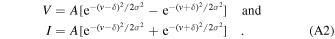
In principle, the amplitudes of RCP and LCP profiles need not be equal. For example, if the velocity coherence along the maser column is different for the two modes, then one component could have a larger amplitude than the other. To cater for the situation with different amplitudes, rather than introduce two amplitudes, A is used as the amplitude of the RCP component, while the LCP amplitude is parameterized using a factor f such that the LCP amplitude is Af. The V and I Stokes components can then be written as
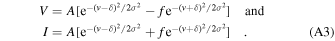
The arguments of the exponential terms can be expanded, giving
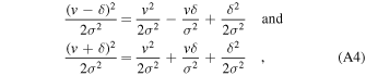
so that the exponential terms can be written in the form
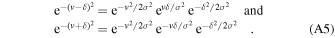
Noting that each term in the expressions for V and I contain the terms  , these terms can be taken outside the brackets and canceled, which leads to
If δ/σ ≪ 1, and v≤σ then vδ/σ2 ≪ 1 so that  can be expanded to first order in a Taylor series to get
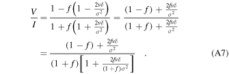
Provided 2fvδ ≪ (1 + f)σ2, V/I can be approximated by
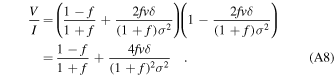
This is a linear function with a slope m = 4fδ/(1 + f)2σ2 that cuts the velocity axis at v = (f − 1)(f + 1)σ2/4fδ. It is straightforward to show that for f = 1

and the V/I line cuts the velocity axis at v = 0 . If there is a significant difference in the amplitudes, then both the slope and the v-axis intersection are affected.
The largest measured value of f from Table 3 is 1.009 for G173, which is the observation with the smallest SNR. Substituting this value into the above formulae changes the velocity intersection from 0 to 0.0004 and the slope is affected by a factor <10−4. In both instances, these factors are less than the uncertainties associated with the derived values and therefore the difference in amplitudes is inconsequential.
Appendix B: Derivative of Stokes I Proportional to Stokes V
From the definition of a derivative, approximate expressions for dI/dv are given by
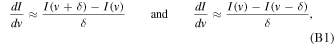
from which it follows that

If RCP and LCP profiles have equal amplitudes, then
which gives
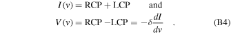
The above derivation requires equal amplitude profiles for RCP and LCP and that δ is small, but sets no criteria for how small δ must be.
Using the two Gaussian maser profile model described in Appendix A, the derivative of the I component with respect to velocity is
where the last equation has been obtained by replacing I/V with Equation (A8). Using this equation, the derivative of I can be computed and fitted to V to determine solutions for both δ and f.
For f = 1 the derivative of the I component simplifies to
which agrees with Equation (B4) with the additional criterion that δ ≪ σ.