Abstract
Solar active regions are believed to provide significant information on the mutual conversion of the poloidal and toroidal components of the global magnetic field. However, the multiscale periodic variations, in particular the quasi-biennial oscillations (QBOs), of solar active regions are not fully understood. In the present study, the flux, area, and number of solar active regions, as well as the sunspot number data in the period from 1996 May to 2023 November, are studied in detail. The multiscale periodic components in the above four data sets are investigated by the techniques of ensemble empirical mode decomposition and cross-correlation analysis. The main results are as follows. (1) The four data sets exhibit similar periodic components, including the 11 yr Schwabe cycle, the QBOs, and a Rieger-type period. (2) The multiscale periodicity of solar active regions shows different physical characteristics. Under different periodic scales, the highest correlation is between active region flux and area, indicating that active region flux and area better reflect the evolution of active regions. (3) By superimposing the QBOs on the 11 yr Schwabe cycle, the Gnevyshev gap phenomenon was clearly observed, implying that the Gnevyshev gap may be caused by the modulation of the 11 yr Schwabe cycle. (4) The active region flux in both hemispheres shows similar periodic components to the full disk, but the periodic variations are uneven between the northern and southern hemispheres. The results of our analysis could be beneficial for the understanding of the spatiotemporal distribution of solar active regions, and could also provide statistical constraints on solar dynamo theories.
Original content from this work may be used under the terms of the Creative Commons Attribution 4.0 licence. Any further distribution of this work must maintain attribution to the author(s) and the title of the work, journal citation and DOI.
1. Introduction
Many solar activity indices exhibit quasi-periodic behaviors, such as sunspots, faculae, plages, filaments, solar flares, coronal jets, and coronal mass ejections. Among these quasi-periodic phenomena, the most prominent periodicity is the 11 yr Schwabe cycle of solar activity (H. Schwabe 1844). Other periodicities have also been identified in many solar activity proxies, including the solar rotation period of about 27 days, the Rieger-type periods of 130–190 days, and the Hale cycle of 22 yr (G. E. Hale 1908; E. Rieger et al. 1984; K. Mursula & B. Zieger 1998). Most researchers believe that the periodic or quasi-periodic behavior of solar activity is driven by the solar dynamo, yet the physical processes governing these solar activity cycles remain poorly understood and are a topic for future exploration (R. H. Cameron & M. Schüssler 2017; A. Biswas et al. 2023; R. Okatev et al. 2023).
Except for the periodicities mentioned above, the most important and notable typical periodicity is the quasi-biennial oscillations (QBOs) of approximately 2 yr (ranging from 0.6 to 4 yr) (A. Vecchio & V. Carbone 2008; G. Bazilevskaya et al. 2014; P. Chowdhury et al. 2019). It is commonly believed that the source region for the QBOs is located in the convective zone (E. E. Benevolenskaya 1998; A. Vecchio & V. Carbone 2008; K. Jain et al. 2023), indicating that its spatiotemporal evolution pattern is closely related to the dynamic processes within the solar interior. Solar QBOs are ubiquitous in the vast amount of observational data available, and they are prevalent in the solar magnetic field, the solar atmosphere, and the interplanetary medium. B. Ravindra et al. (2022) utilized wavelet techniques to analyze the data of sunspot number and area from Solar Cycles 14–24 at Kodaikanal Observatory, revealing QBOs with periods ranging from 1.5 to 2.5 yr. P. Chowdhury et al. (2022) explored various midterm periods of the Ca-K index using power spectral analysis, finding significant 1.2–1.4 yr QBOs in data from the northern hemisphere and the full solar disk during Solar Cycles 15–21. J. D. Richardson et al. (1994) detected strong variations in solar wind speed on a timescale of 1.3 yr based on long-term studies of auroras and magnetometers.
The physical mechanism of the QBOs remains unclear, but most researchers believe it to be an intrinsic feature of the solar dynamo mechanism (R. Howe et al. 2000; M. Laurenza et al. 2012; I. H. Cho et al. 2014). To reveal the QBOs in solar magnetic activity, E. E. Benevolenskaya (1998) proposed two dynamos operating at different locations: one at the base of the convection zone and the other in a region 5% below the photosphere. The characteristics of solar QBOs and helioseismic data may be related to the interaction between these two dynamo mechanisms at different depths (S. T. Fletcher et al. 2010; K. Jain et al. 2011, 2023). E. Covas et al. (2000) explained the generation of QBOs using a spatiotemporal fragmentation mechanism. At the base of the convection zone, spatiotemporal fragmentation occurs under specific magnetohydrodynamic conditions, creating oscillations in differential rotation that lead to the formation of QBOs. A random effect is also a possible mechanism for solar QBOs; Y. M. Wang & N. R. Sheeley (2003) simulated results that produced peaks related to solar QBOs, with the highest peak potentially appearing during the declining phase and maximum of the solar cycle. R. Simoniello et al. (2013) suggested that the beating between dipole and quadrupole magnetic fields could also cause solar QBOs. Additionally, the instability of magnetic Rossby waves is considered one of the driving mechanisms of solar QBOs. The differential rotation and magnetic field strength within the Sun vary over the solar cycle, leading to the instability of magnetic Rossby waves, which in turn triggers periodic variations (Y.-Q. Lou 2000; P. Chowdhury et al. 2009; L. H. Deng et al. 2020b; T. V. Zaqarashvili et al. 2021; M. B. Korsós et al. 2023).
The long-term evolution of solar activity indices in the northern and southern hemispheres exhibits significant asynchronous asymmetry. This phenomenon reveals differences in the strength and phase of the solar cycle between the two hemispheres, which is crucial for understanding the mechanism of the solar magnetic field (O. G. Badalyan & V. N. Obridko 2011; A. A. Norton et al. 2014; X. Zhang et al. 2024). Extensive research has been performed on the hemispheric asymmetry of periodic variations across different timescales. For example, E. Gurgenashvili et al. (2017) found significant hemispheric asymmetry in the Rieger-type periodicity of sunspot number and sunspot area, suggesting it may be caused by magnetic Rossby waves in the solar internal dynamo. L. H. Deng et al. (2019) reported complex phase relationships in the solar QBOs of the Hα flare index between the northern and southern hemispheres and discussed their possible origin. Therefore, hemispheric asymmetry is an essential characteristic of periodic variations in solar activity.
Active regions (ARs) are areas of strong magnetic field on the Sun, originating from the solar internal dynamo process, and exhibit complex spatial and temporal behavior from the photosphere to the corona (T. Zhang et al. 2024). However, the investigation of ARs has mainly concentrated on the detection (J. Zhang et al. 2010; I. Sukarsih et al. 2020; L. Gong et al. 2024), classification (S. A. Jaeggli & A. A. Norton 2016; W. Mohamed et al. 2018; V. I. Abramenko et al. 2023), and analysis of individual ARs (R. A. Schwartz & B. R. Dennis 1989; A. Joshi 1993; P. Jaswal et al. 2025), with limited studies on their periodicity. T. B. Goldvarg et al. (2005) studied the periodicity of energy release in ARs by analyzing flare data in the maximum of Solar Cycle 21 and discovered the existence of some short-period oscillations. Y. A. Nagovitsyn & A. I. Kuleshova (2013) studied the flare recurrence in ARs during Solar Cycle 23 and found that the number of flares in an AR is closely related to the sunspot area and the flare energy release rate in that region. G. Dumbadze et al. (2017) discovered characteristic periodic oscillations of 4.9 and 4.6 hr in the inclination angle data through the study of two ARs, which can be explained by fast and slow kink modes. G. Dumbadze et al. (2021) investigated low-frequency oscillations in solar ARs and found oscillations in the total area and radial flux of ARs with periods ranging from 2 to 20 hr; no periodicity was found in the inclination angle data. Therefore, research on the multiscale periodicity of ARs is relatively limited and it requires further investigation.
In this paper, we utilize the database of ARs created by R. Wang et al. (2024) to study the multiscale periodic variation of solar ARs during the time interval 1996–2023. Next, Section 2 briefly introduces the data set and the methods used in this paper. Section 3 analyzes the solar QBOs and their relationship with the phases of the three parameters and the sunspot number. Finally, a summary and discussion are provided in Section 4.
2. Data and Methods
2.1. Solar ARs
In this study, the multiscale periodic variations in solar ARs are examined using the live homogeneous database of ARs8 provided by R. Wang et al. (2023, 2024). They developed a method for automatically detecting and calibrating solar ARs based on the Michelson Doppler Imager on board the Solar and Heliospheric Observatory (SOHO/MDI; P. H. Scherrer et al. 1995) and the Helioseismic and Magnetic Imager on board the Solar Dynamics Observatory (SDO/HMI; P. H. Scherrer et al. 2012), with synoptic magnetograms from the Joint Science Operations Center.9
This study follows the method reported by W. Thompson (2006). The Carrington rotation (CR) number and label are jointly used to uniquely identify an AR, converting the CR into calendar dates to determine the occurrence time of each AR. To analyze the periodic variations of ARs, we first convert the CR number of each AR into its corresponding calendar date (with CR 1 starting on 1853 November 9), which serves as the occurrence time of the AR. Then we accumulate the ARs that appear within the same month and use this as monthly data, with subsequent work based on the monthly data. The database currently provides data on ARs from CR 1909 to 2278, corresponding to 1996 May through 2023 November and spanning two complete solar cycles, Cycles 23 and 24, as well as part of Solar Cycle 25. We selected three basic parameters of solar ARs from this database: flux, area, and number. Studying the periodic variations of solar ARs through this database will contribute to a deeper understanding of the periodic changes in the solar magnetic field.
2.2. International Sunspot Number
To investigate the relationship between sunspot activity and ARs, we used the monthly sunspot numbers covering the period from 1996 May to 2023 November from the World Data Center. They can be obtained from SILSO.10
Figure 1 displays the temporal variations of the three AR parameters and the sunspot number for the time interval from 1996 May to 2023 November. The black solid line shows the raw data, while the red solid line represents the 13 month smoothed data. As can be seen in the figure, the three fundamental parameters of AR flux, area, and number, as well as sunspot number, exhibit distinct periodicity. After smoothing these data, we found that a double-peaked structure appears in each solar cycle. However, a distinct anomaly is observed in Solar Cycle 23: the first peak value of the AR flux, area, and sunspot number is smaller than the second peak, while the first peak of the AR number is higher than the second. The objective of this study is to conduct a further analysis of the periodicity in these data to uncover the underlying mechanisms and patterns in solar activity.
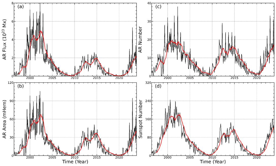
Figure 1. Monthly values of solar AR flux, area, number, and sunspot number for the time interval from 1996 May to 2023 November.
Download figure:
Standard image High-resolution image2.3. Empirical Mode Decomposition
Various authors have employed different methodologies for time–frequency analysis to investigate the periodicities of solar activity (V. M. Nakariakov et al. 2010; M. Stangalini et al. 2014; Z.-N. Qu et al. 2015). The empirical mode decomposition (EMD), also known as the Hilbert–Huang transform and proposed by N. E. Huang et al. (1998), is a technique for analyzing nonlinear and nonstationary time series. It decomposes the data based on its own temporal scale characteristics, without the need to predetermine basis functions. This hallmark of the EMD method fundamentally differentiates it from traditional Fourier methods and wavelet transform techniques. Consequently, the EMD method is theoretically capable of decomposing any type of signal, which establishes it as a potent analytical tool with extensive applications in a multitude of scientific disciplines (D. Y. Kolotkov et al. 2016; Y. Su et al. 2017; T. Mehta et al. 2022; Y. Yuan et al. 2024; W. Zhong et al. 2024).
The EMD method proficiently decomposes a complex input signal into a finite collection of intrinsic mode functions (IMFs) that embody physical significance. These IMF components capture the local characteristic signals of the original signal on various temporal scales. The characteristic timescale of the IMF extracted by EMD is based on the local distance between two consecutive extrema, meaning that each IMF represents a potential oscillatory mode, which is locally defined and therefore nonstationary.
Given an input signal x(t), the EMD method decomposes it into several IMFs along with a residual component r(t). This can be expressed in the following formula (M. J. Käpylä et al. 2016):
where n is the total number of IMFs. An IMF must satisfy two conditions: (a) the function must have an equal number of local extrema and zeros or a difference of at most one over the entire time range, and (b) at any moment, the local upper and local lower envelopes must be zero on average. The process of extracting IMFs is referred to as sifting, and proceeds as follows: (i) identify the local maxima and minima of the input signal, (ii) connect the maxima with cubic spline interpolation to form the upper envelope, and the minima to form the lower envelope, then compute the mean of the upper and lower envelopes, and (iii) subtract the mean of the upper and lower envelopes from the input signal to obtain a new signal. If the new signal still contains negative local maxima and positive local minima, this indicates that it is not yet an IMF, and thus the new signal should be returned as the input for step (i) to continue the sifting process. The sifting stops when r(t) is a monotonic function or a constant value.
2.4. Ensemble Empirical Mode Decomposition
Due to the mode mixing problem that occurs during the execution of the EMD, there may exist signals with a wide range of scales but different characteristics within the same IMF component, as well as signals with similar scales across different IMF components. This mode mixing can cause the IMFs to lose their unique scale characteristics, making their physical significance unclear. To overcome the limitations of EMD, particularly mode mixing, Z. Wu & N. E. Huang (2009) devised a noise-assisted enhancement called ensemble empirical mode decomposition (EEMD). This method involves decomposing white noise with EMD and then performing statistical analysis on the output.
The core of the EEMD method is to superimpose Gaussian white noise with multiple EMDs, taking advantage of the statistical properties of Gaussian white noise with uniformly distributed frequencies. At each processing, different instances of white noise with the same amplitude are added to change the characteristics of the signal’s extrema. Subsequently, the IMFs derived from these multiple EMD processes are subjected to an averaging procedure, which serves to counteract the influence of the added white noise, thereby significantly mitigating the incidence of mode mixing. Many authors have used this method to investigate the presence of periodicities in the solar activity index (M. Zapiór et al. 2016; Y. Mei et al. 2018; L. H. Deng et al. 2019; J. Wang et al. 2022).
The steps in the EEMD operation are as follows: (i) Gaussian white noise is introduced into the original signal, (ii) the resultant noisy signal is treated as a composite entity and subjected to EMD, thereby yielding a series of IMF components, (iii) steps (i) and (ii) are iteratively executed, each time with a newly generated sequence of normally distributed white noise, and (iv) the IMFs obtained from each iteration are subjected to an ensemble averaging process to yield the final result.
There are two critical parameters in the EEMD method: the standard deviation of the white-noise sequence and the number of noise additions. The amplitude of the noise determines the intensity of the noise introduced into the original signal. If the noise amplitude is too high, the resulting IMF components may become distorted; conversely, if the noise amplitude is too low, it may fail to effectively address the issue of mode mixing. The number of noise additions dictates how many times the original signal undergoes the EMD. Increasing the number of noise additions can enhance the stability and robustness of the EEMD algorithm, but it also increases the computational burden. In this study, white-noise sequences with standard deviations ranging from 0.02 to 0.4 (in steps of 0.02, totaling 20 cases) were added, with the noise added 100 times.
Many statistical analysis techniques are used to study the phase relationships between solar indices (A. Kilcik et al. 2010; J. Muraközy 2016; J. Oloketuyi et al. 2019; Y.-Y. Li et al. 2022). Cross-correlation analysis (CCA) can be employed to assess the degree of correlation between two time series. To examine the phase relationships of AR flux, area, and number, as well as sunspot number in QBOs, this study has chosen the method of CCA. To calculate the correlations between pairs of parameters, we utilized MATLAB code to compute the correlation coefficients (CCs) and subsequently analyzed the obtained coefficients. To assess the statistical significance in the CCA, we calculated the 95% confidence levels using the Bartlett formula (M. S. Bartlett 1946). Considering the complexity of the solar data, these confidence levels are interpreted qualitatively. It should be noted that in this paper, all phase lags and time intervals in the CCA are expressed in months.
3. Analysis and Result
3.1. Periodic Modes of ARs and Sunspot Number
By employing the EEMD technique, six IMFs and a trend component were extracted for each data set within the time considered. Given that white noise was introduced and varied in 20 steps, each IMF corresponds to 20 distinct time series. Within the temporal range considered, the final IMFs are derived as the means of these 20 time series. Figure 2 displays the decomposition results of AR flux and area, and Figure 3 shows AR number and sunspot number. Both figures are structured with subplots arranged sequentially from top to bottom and show the IMFs by frequency from high to low, with the last subplot showing the corresponding trend.
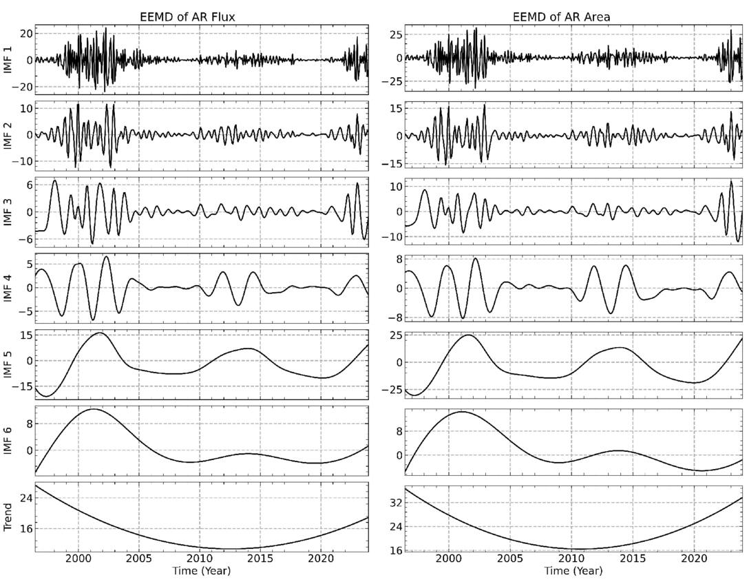
Figure 2. The average IMFs of AR flux (1022 Mx) and area (mHem, or millihemispheres). The panels display IMFs 1–6 and the trend in order from top to bottom.
Download figure:
Standard image High-resolution image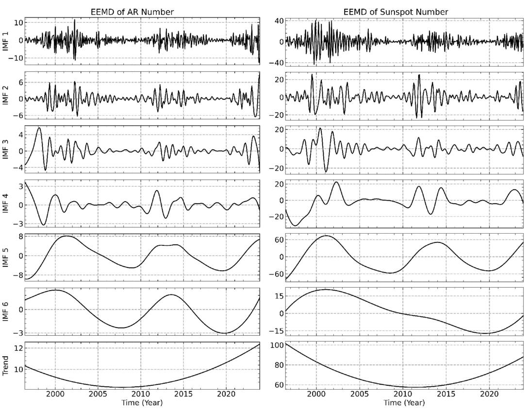
Figure 3. The average IMFs of the AR number and the sunspot number. The panels display IMFs 1–6 and the trend in order from top to bottom.
Download figure:
Standard image High-resolution imageTo illustrate the decomposition results of the EEMD technique with varying standard deviations of white-noise sequences, we take the IMF4 components extracted from AR flux, area, and number, as well as the sunspot number, as an example. Figure 4 displays the time series of IMF4 for all four data sets. In each panel, the 20 black lines represent the added white-noise standard deviations ranging from 0.02 to 0.40 in increments of 0.02, while the red line indicates the average of the 20 time series. Z. Wu & N. E. Huang (2009) believe that after adding white noise with finite amplitude, the decomposition results of the data using EEMD are usually only slightly affected by changes in the noise amplitude. It is clear from Figure 4 that the results of the 20 different white-noise sequence decompositions exhibit good synchronization, indicating that the results obtained by the EEMD method are stable. The EEMD improves on the original EMD by adding white noise to decompose signals, reducing the issue of mode mixing and enhancing robustness against noise, thus allowing for clearer extraction of features within the IMFs.
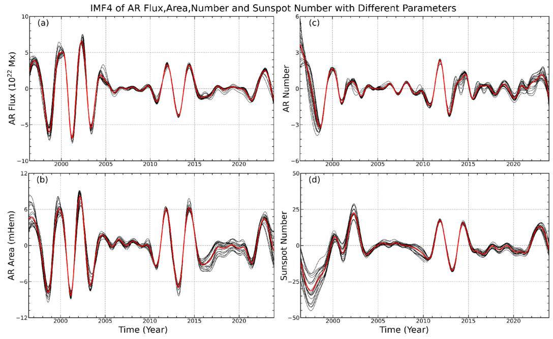
Figure 4. IMF4 of (a) AR flux, (b) area, and (c) number, as well as (d) sunspot number. In each panel, 20 black lines represent the results of the EEMD algorithm with added noise, varying in standard deviation from 0.02 to 0.40 in increments of 0.02. The bold red line indicates the average IMF4 calculated from the 20 time series. Each case is based on an ensemble of 100.
Download figure:
Standard image High-resolution imageBased on the EEMD method, the average periodicities of IMFs 1–6 for AR flux, area, number, and sunspot number were calculated, and the results are listed in the second to fifth columns of Table 1. As shown in Figures 2 and 3, the IMF5 extracted from each data set represents the 11 yr Schwabe cycle. The calculated average periodicities of the IMF5 for the AR flux, area, number, and sunspot number are 11.125 ± 0.013, 11.083 ± 0.125, 11.083 ± 1.147, and 11.500 ± 0.152 yr, respectively.
Table 1. Average Periodicities of the Six IMFs Derived from the AR Flux, Area, Number, and Sunspot Number
| AR Flux | AR Area | AR Number | Sunspot Number | |
|---|---|---|---|---|
| (year) | (year) | (year) | (year) | |
| IMF1 | 0.209 ± 0.001 | 0.243 ± 0.002 | 0.266 ± 0.002 | 0.341 ± 0.004 |
| IMF2 | 0.525 ± 0.002 | 0.531 ± 0.011 | 0.696 ± 0.009 | 0.735 ± 0.165 |
| IMF3 | 1.121 ± 0.032 | 1.171 ± 0.026 | 1.121 ± 0.008 | 1.062 ± 0.009 |
| IMF4 | 2.526 ± 0.013 | 2.582 ± 0.066 | 2.785 ± 0.494 | 3.070 ± 0.107 |
| IMF5 | 11.125 ± 0.013 | 11.083 ± 0.125 | 11.083 ± 1.147 | 11.500 ± 0.152 |
| IMF6 | 12.333 ± 5.787 | 13.250 ± 6.646 | 13.333 ± 0.214 | ... |
Download table as: ASCIITypeset image
IMF1 may mainly represent high-frequency noise, as monthly AR data were used in this study (B. L. Barnhart & W. E. Eichinger 2011). Moreover, IMF6 shows a signal in the AR parameters that is close to the 11 yr Schwabe cycle, but with noticeable errors. These discrepancies may be attributed to both the characteristics of the EEMD method and the nature of the AR data. The sunspot number is a classic indicator of solar activity and has undergone multiple revisions. In particular, its 11 yr cycle has been widely validated. In contrast, AR parameters are derived from SOHO/MDI and SDO/HMI observations, which lack long-term joint observations from multiple telescopes. Furthermore, ARs reflect more complex information. As a result, IMF6 was extracted from the three AR parameters, but not from the sunspot number. In the future, data from longer time series may help verify the existence of IMF6 in the sunspot number.
An oscillation pattern with period in the range 0.525 to 0.735 years in IMF2 has been obtained by many authors using different solar activity indices, such as sunspot area, X-ray flares, and sunspot groups (Y.-Q. Lou et al. 2003; P. Chowdhury et al. 2009; A. Kilcik et al. 2010). In this study, we consider the IMF2 as a Rieger-type period. The Rieger-type period of 154 days is not a permanent feature of solar activity, but varies with the solar cycle. Many researchers believed that the Rieger-type period may be related to magnetic Rossby waves in the solar tachocline (J. Zhang et al. 2010; M. B. Korsós et al. 2023). Recently, S. W. McIntosh et al. (2017) performed an analysis using observations of coronal bright points from the Solar Terrestrial Relations Observatory (STEREO) and SDO, and their results provided strong evidence that magnetic Rossby waves are the mechanism for the generation of the Rieger-type period. The Rieger-type period was once thought to be a harmonic of the solar rotation period. This oscillation mode is close to the subharmonic period of 25–26 days, which is near the rotation period of the solar equator (T. Bai & E. W. Cliver 1990). Based on this, T. Bai & P. A. Sturrock (1991) proposed a hypothesis that a fundamental period may give rise to the occurrence of subharmonic oscillations. A. Özgüç & T. Ataç (1996) reported a fundamental period of 25.5 days when studying the north–south asymmetry of flares during Solar Cycle 22, with other periods also close to integer multiples of 25.5 days.
The average periodicities of IMF3 and IMF4 are associated with a typical timescale of approximately 2 yr, so IMF3 and IMF4 can be considered as QBOs. The amplitude of solar QBOs changes over time, and this variation exhibits a random characteristic, a phenomenon known as the intermittency of the solar QBOs (Y. M. Wang & N. R. Sheeley 2003; G. Bazilevskaya et al. 2014; G. A. Bazilevskaya et al. 2015; Y.-w. Qian et al. 2019). To study the differences between IMF3 and IMF4 in different solar cycles, we used the continuous wavelet transform proposed by C. Torrence & G. P. Compo (1998) to analyze the local variations of IMF3 and IMF4 for the four parameters in the time interval considered. The results are shown in Figures 5 and 6. In the upper panels of Figures 5 and 6, the thick black contour lines represent the 95% confidence level, and the black dashed lines represent the cone of influence (COI), within which edge effects may have some impact on the results. The two vertical red lines in each plot divide the time into Solar Cycles 23, 24, and 25. In the bottom panel, the corresponding local wavelet power spectrum is shown, with the 95% confidence level marked by black dashed lines.
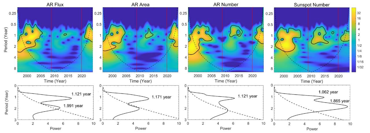
Figure 5. Upper panels: continuous wavelet power spectra of IMF3 for AR flux, AR area, AR number, and sunspot number. The thick black contour lines represent the 95% confidence level, and the black dashed lines represent the cone of influence, within which edge effects may influence the results. The two vertical red lines in each plot divide the time into Solar Cycles 23, 24, and 25. Bottom panels: global wavelet power spectra corresponding to IMF3 for the four parameters within the considered time range, along with the 95% confidence level (dashed line).
Download figure:
Standard image High-resolution image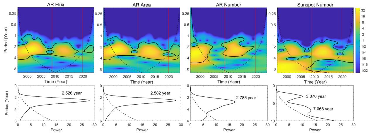
Figure 6. Upper panels: continuous wavelet power spectra of IMF4 for AR flux, AR area, AR number, and sunspot number. The thick black contour lines represent the 95% confidence level, and the black dashed lines represent the cone of influence, within which edge effects may influence the results. The two vertical red lines in each plot divide the time into Solar Cycles 23, 24, and 25. Bottom panels: global wavelet power spectra corresponding to IMF4 for the four parameters within the considered time range, along with the 95% confidence level (dashed line).
Download figure:
Standard image High-resolution imageFrom Figures 5 and 6, it can be clearly seen that solar QBOs occur mainly during solar activity maxima, while they are relatively weak or nearly nonexistent during solar minima. This variation pattern of QBOs is consistent with previous research findings (L. H. Deng et al. 2019; B. Ravindra et al. 2022; K. Jain et al. 2023). Figure 5 shows the variation characteristics of IMF3 for four parameters within the time range considered. In the wavelet power spectrum, distinct significant power values are observed between Solar Cycles 23 and 24. The periodic fluctuations of the four IMF3 components are stronger during Solar Cycle 23 than during Solar Cycle 24. This difference may be due to the disparity in intensity of solar activity between the two solar cycles. Solar activity was stronger during Solar Cycle 23 than Solar Cycle 24, resulting in higher power concentration and a wider fluctuation range in the periodic oscillations during Solar Cycle 23. Through the global wavelet power spectrum, we observe that all four parameters exhibit a double-peak structure, but only the double peaks of AR flux and sunspot number are significantly present at the 95% confidence level. Moreover, the second peak appears only in Solar Cycle 23. This indicates that the solar QBOs with a period of less than 2 yr exhibit a noticeable difference between Solar Cycles 23 and 24. In Figure 6, we observe that the fluctuations of sunspot number exhibit a more complex pattern than AR flux, area, and number. This may be due to the characteristics of the original data. Additionally, solar QBOs with a period greater than 2 yr exist in both Solar Cycles 23 and 24. K. Jain et al. (2023) reported that the approximately 2 yr QBO dominates in Solar Cycle 23, while the approximately 3 yr solar QBO dominates in Solar Cycle 24. The results in this study partially support the findings of K. Jain et al. (2023).
3.2. Phase Relationships of the Rieger-type Period
Pairwise cross-correlation analysis was conducted on the four IMF2 time series obtained from the EEMD, and the phase relationship was determined by the time lag when the two time series reach their peak values. The results are shown in Figure 7 and Table 2. The abscissa represents the phase lag of the former with respect to the latter, with positive values indicating a forward lag, which means that the former reaches its peak after the latter (M. Hagino et al. 2004; A. Kilcik et al. 2017; L. H. Deng et al. 2020a). The vertical coordinate represents the CC between the two time series. The red dashed line is used to estimate the statistical significance of the CC, with most local peaks exceeding the 95% confidence level, similar to Figures 8 and 9.
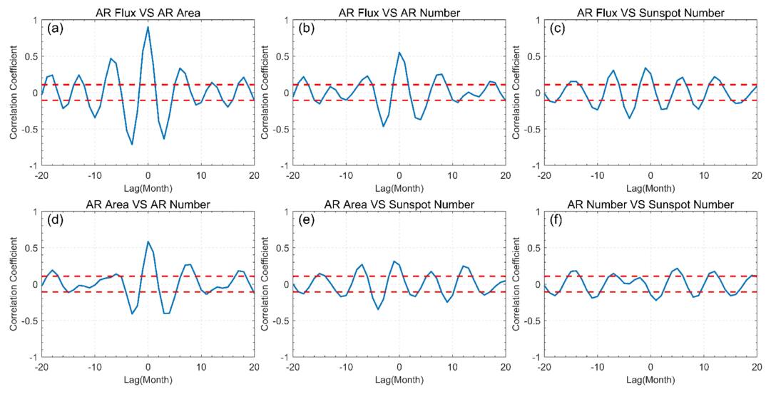
Figure 7. CCA results of IMF2 between the AR flux, area, number, and sunspot number. The red dashed line indicates the 95% confidence level.
Download figure:
Standard image High-resolution imageTable 2. Values of the CC and Their Corresponding Phase Lag (in Months)
| IMF2 | IMF4 | IMF3 + IMF4 | IMF5 | ||||||||
|---|---|---|---|---|---|---|---|---|---|---|---|
| CC | Phase Lag | CC | Phase Lag | CC | Phase Lag | CC | Phase Lag | ||||
| AR flux vs AR area | 0.900 | 0 | 0.959 | 1 | 0.945 | 0 | 0.984 | 1 | |||
| AR flux vs AR number | 0.551 | 0 | 0.761 | 1 | 0.620 | 0 | 0.902 | 1 | |||
| AR flux vs sunspot number | 0.337 | −1 | 0.407 | 0 | 0.496 | −1 | 0.858 | 2 | |||
| AR area vs AR number | 0.584 | 0 | 0.787 | 0 | 0.599 | −1 | 0.921 | 0 | |||
| AR area vs sunspot number | 0.313 | −1 | 0.510 | 0 | 0.496 | −1 | 0.899 | 1 | |||
| AR number vs sunspot number | 0.216 | 5 | 0.369 | 1 | 0.332 | −28 | 0.922 | 0 | |||
Download table as: ASCIITypeset image
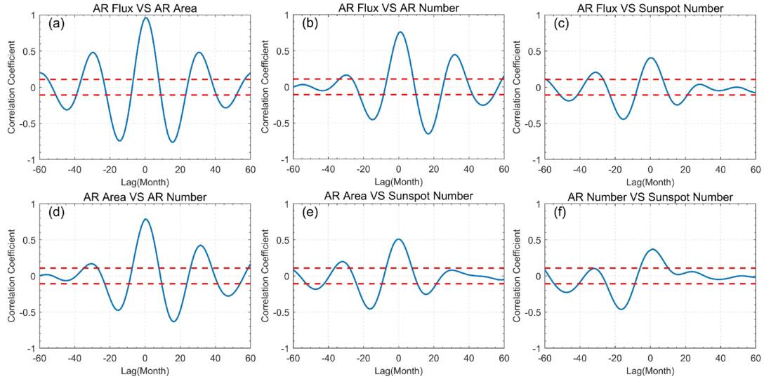
Figure 8. CCA results of IMF4 between the AR flux, area, number, and sunspot number. The red dashed line indicates the 95% confidence level.
Download figure:
Standard image High-resolution image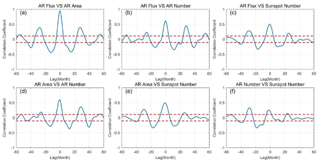
Figure 9. CCA results of superimposing IMF3 and IMF4 between the AR flux, area, number, and sunspot number. The red dashed line indicates the 95% confidence level.
Download figure:
Standard image High-resolution imageThrough the CCA, we found that the CC between AR flux and AR area is 0.900, with a phase lag of 0, which is the highest among the six CCs. Among the AR parameters, the CC between AR flux and AR number is the lowest, at only 0.551. In contrast, the correlation between the AR parameters and sunspot number is much weaker. The CC between AR number and sunspot number is only 0.216, with a phase lag of 5 months, meaning that the sunspot number leads the AR number by 5 months to reach its peak. This suggests a poor synchronization of the variation patterns between AR number and sunspot number on the Rieger-type periodic scale. Since the Rieger-type period is generally associated with solar tachocline nonlinear oscillations and magnetic Rossby wave instability (M. Dikpati et al. 2018; M. B. Korsós et al. 2023), this weaker correlation may reflect the inconsistency in the response of different layers of solar dynamical mechanisms to each parameter.
3.3. Phase Relationships of Solar QBOs
3.3.1. Phase Relationships of IMF4
Figure 8 presents the results of the pairwise CCA between AR flux, area, number, and sunspot number for IMF4, with phase lags spanning from −60 to +60 months. The corresponding phase lags and CCs are listed in Table 2 for the four IMF4 pairwise CCA analyses.
As shown in Figure 8(a), the two time series of the AR flux and area reach their maximum CC of 0.959 when the phase lag is 1 month, indicating a positive correlation between their IMF4s globally. Within the time range of −60 to +60 months, there are three local maxima in the cross-correlation plot. The CCs reach local maxima of 0.481, 0.959, and 0.483 when the phase lags are −30, 1, and 31 months, respectively. The average interval between two adjacent local maxima is 30.75 months. When the relative phase lags are −45, −14, 16, and 46 months, the CCs reach local minima of −0.311, −0.742, −0.761, and −0.286, respectively. The average interval between two adjacent local minima is 30.33 months. Figure 8(b) shows the results of the CCA between the AR flux and number. Similarly to the analysis between the AR flux and area, the AR number leads the AR flux by 1 month to reach its peak, with a CC of 0.761. In the time range from −60 to +60 months, the cross-correlation plot shows three local maxima. The phase lags at which the local maxima occur are −30, 1, and 32 months, with the average interval between two adjacent local maxima being 31.33 months. At the same time, when the phase lags are −15 and 17 months, local minima are reached, with an average interval of 32 months between them. Figure 8(c) presents the CCA between the AR flux and the sunspot number. Globally, the CC reaches its maximum value of 0.407 when the phase lag is 0. Over the range of phase lag from −60 to +60 months, there are two local maxima and three local minima. The interval between two adjacent local maxima is 31 months, while the average interval between two adjacent local minima is 30.5 months. From the above analysis, it can be concluded that the AR flux is positively correlated with the AR area, number, and the sunspot number, with the strongest correlation between the AR flux and area. It is noteworthy that the IMF4 of the AR area and number peaks one month ahead of the AR flux, while there is no phase difference between the AR flux and the sunspot number.
Figures 8(d) and (e) display the CCA results between the AR area and number, and between the AR area and the sunspot number, respectively. In both cases, the maximum CC occurs with a phase lag of zero. However, the CC for the IMF4 between the AR area and number is 0.787, while that between the AR area and the sunspot number is lower, at 0.510. For IMF4 between the AR area and number, the average interval between two adjacent local maxima (minima) is 31.66 (31) months, whereas for IMF4 between the AR area and the sunspot number, the average interval between two adjacent local maxima (minima) is 32 (31.5) months. Finally, Figure 8(f) presents the CCA result between the AR number and the sunspot number for IMF4. The maximum CC of 0.3689 occurs at a phase lag of 1 month, while all other local maxima are below the 95% confidence level. At phase lags of −48 and −16 months, the CCs are −0.228 and −0.462, respectively, with an interval of 32 months between them.
In conclusion, there is a positive correlation between the AR flux, area, number, and the sunspot number. Among these, the correlation between the AR flux and area is the strongest, while the CCs between the three AR parameters and the sunspot number are relatively low, indicating that there are differences between the characteristics of ARs and sunspots in QBOs.
3.3.2. Phase Relationships of IMF3 and IMF4
Since we consider IMF3 and IMF4 as the solar QBOs, we will next perform CCA between the AR flux, area, number, and the sunspot number after superimposing IMF3 and IMF4. The CCA results are shown in Figure 9, with phase differences and CCs between each pair of parameters listed in Table 2 for the time lags ranging from −60 to 60 months. Figures 9(a)–(c) display the results of the pairwise CCA between the AR flux and area, number, and sunspot number. Globally, the lag times are 0, 0, and −1 month, and the CCs are 0.945, 0.620, and 0.496, respectively. In the range from −60 to 60 months, the average length between adjacent local maxima of the AR flux and area is 27.5 months, and between local minima it is 26.66 months. The average lengths between adjacent local maxima and minima of the AR flux and number are 27.25 and 26.5 months, respectively, and those between the AR number and sunspot number are 27 and 24.66 months.
The results between the AR area and the number, and the sunspot number, are shown in Figures 9(d) and (e). The CC between the AR area and the number reaches its maximum value of 0.599 at a lag of −1 month, with the average lengths between adjacent local maxima and minima being 27.5 and 26 months, respectively. Similarly, the CC between the AR area and the sunspot number also reaches its maximum value of 0.496 at a lag of −1 month, with the average lengths between adjacent local maxima and minima being 27.5 and 26 months, respectively. The CCA results between AR number and sunspot number are shown in Figure 9(f), where the CC is 0.332 with a lag of −28 months, with the average lengths between adjacent local maxima and minima being 26 and 22.5 months, respectively.
Comparing Figures 8 and 9, it can be observed that the contour in Figure 8 is smoother and better than the one in Figure 9. When comparing IMF4 in Table 2 with the combination of IMF3 and IMF4, it is found that the former has a higher CC than the latter, except for the AR flux and number. That means that the CCs of solar QBOs for the AR flux, area, number, and the sunspot number are higher when only IMF4 is considered. It should be noted that the period range of the solar QBOs is defined differently by different researchers, but it is generally considered that oscillations with a period of around 2 yr (between 1 and 3 yr) are referred to as solar QBOs (K. Mursula & B. Zieger 2000; Y. M. Wang & N. R. Sheeley 2003; N. Gyenge et al. 2014). The reason for the occurrence of this phenomenon may be that part of the time range of IMF3 falls outside the definition of QBOs, and some researchers believe that the approximately 1 yr periodicity is related to the signal of annual temperature variation. This 1 yr periodicity has been observed in many solar indices, such as the total solar irradiance, the average solar magnetic field, and the full-disk solar magnetic field (V. A. Kotov 2006; N. B. Xiang & Z. N. Qu 2016). The origin of this cycle remains uncertain, but it is also possible that it is induced by the orbital motion of the Earth, resulting in a 1 yr periodicity (J. Javaraiah et al. 2009).
3.4. Phase Relationships of the 11 yr Schwabe cycle
To compare the relationship of solar AR and sunspots on different timescales, we analyzed the IMF5, which corresponds to the 11 yr Schwabe cycle, and conducted CCA on AR flux, area, number, and sunspot number. The CCs and corresponding phase lags are shown in Table 2. Figures 10(a)–(c) show the CCA between AR flux and area, number, and sunspot number, respectively. From the figures, it can be seen that the maximum CCs for AR flux with area and number occur at a phase lag of 1 month, with values of 0.984 and 0.902, respectively. This indicates that AR flux lags behind the 11 yr Schwabe cycles of area and number by 1 month to reach its peak. AR flux also lags behind the 11 yr Schwabe cycle of sunspot number by 2 months, with a CC of 0.858. Figures 10(d) and (e) show the CCA results between AR area and number, and between AR area and sunspot number, respectively. The results show that there is no phase difference between AR area and number, but a phase difference of 1 month exists between the AR area and sunspot number, with CCs of 0.921 and 0.899, respectively. Moreover, Figure 10(f) shows that there is no phase difference between AR number and sunspot number, with a CC of 0.922.
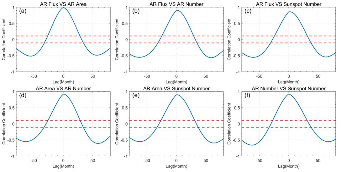
Figure 10. CCA results of IMF5 between the AR flux, area, number, and sunspot number. The red dashed line indicates the 95% confidence level.
Download figure:
Standard image High-resolution imageThrough pairwise CCA of the time series of the three AR parameters and the sunspot number over four 11 yr Schwabe cycles, it was found that the maximum CC occurs between the AR flux and area, reaching 0.984. Since the CC between the AR flux and area is also the highest when analyzing the phase relationship of QBOs, this suggests that the AR flux and area are better indicators of the AR evolution.
The significantly higher CCs in IMF5 suggest that the long-term evolution of AR parameters and sunspot number is modulated by a global dynamo mechanism (R. H. Cameron et al. 2017). This coherent behavior indicates a strong coupling among these indicators during the Schwabe cycle. In contrast, the Rieger-type period and QBOs show weaker correlations, which may reflect the influence of more localized or shallow-layer processes, such as Rossby wave interactions or tachocline dynamics (T. V. Zaqarashvili et al. 2010; M. Dikpati et al. 2018; K. Jain et al. 2023). These differences highlight the distinct physical origins of periodicities at different timescales in the modulation of solar activity.
In addition, CCAs at different periodic scales all indicate a strong correlation between AR flux and AR area, suggesting that both may be jointly regulated by variations in the magnetic field strength of the AR. In contrast, although the AR number is also an AR parameter, it may be influenced by the magnetic structure and energy release of the ARs, resulting in a relatively lower correlation with AR flux and area.
3.5. Superposition of the QBOs and the 11 yr Schwabe Cycle
To explore the relationship between the solar QBOs and the Schwabe cycle, the superposition of IMF4 and IMF5 for each data set is shown in Figure 11, and represents the combination of the solar QBOs with the Schwabe cycle. The red dashed lines indicate the division of time into Solar Cycles 23, 24, and 25. The superposition reveals a distinct double-peaked structure, with all four subplots exhibiting two peaks and a gap, known as the Gnevyshev gap (M. N. Gnevyshev 1967, 1977). This suggests that the Gnevyshev gap is actually the result of the modulation of solar QBOs by the 11 yr Schwabe cycle (M. Laurenza et al. 2012; M. Wan et al. 2020). G. A. Bazilevskaya et al. (2000) identified a distinct slit-like structure in the solar index, characterized by two peaks, and proposed that the amplitude of the solar QBOs is related to the 11 yr Schwabe cycle. A. Vecchio et al. (2012) examined the role of QBOs in the intensity of galactic cosmic rays and demonstrated that the QBOs are indeed the cause of the Gnevyshev gap. The results we obtained are in agreement with theirs, further confirming that the Gnevyshev gap is closely related to solar QBOs and the 11 yr Schwabe cycle.
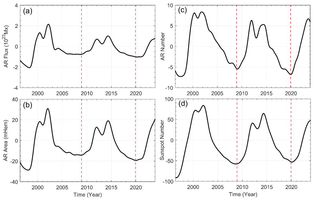
Figure 11. Superposition of the QBO modes and the 11 yr Schwabe cycle of the AR flux, area, number, and sunspot number. The red dashed lines indicate the division of time into Solar Cycles 23, 24, and 25.
Download figure:
Standard image High-resolution imageHowever, it is worth noting that in Solar Cycle 24, the first peak of the AR flux, area, and sunspot number is smaller than the second peak, while for the AR number, the first peak is larger than the second. This suggests that the AR number does not accurately represent the evolutionary behavior of solar ARs.
3.6. Periodic Variations in Hemispheric ARs
3.6.1. Periodic Modes of Hemispheric ARs
The north–south asymmetry plays a crucial role in the evolution of solar magnetic activity, exerting a profound influence on the global dynamo. To gain deeper insights into the manifestations of this asymmetry on different timescales, we analyzed periodic variations in ARs between the northern and southern hemispheres. Using the same decomposition method as the previous section, we selected AR flux to analyze hemispheric periodic variations, as magnetic flux directly represents the magnetic strength and energy of ARs, enabling better characterization of solar magnetic activity (S. Toriumi et al. 2017; V. Archontis & P. Syntelis 2019; A. Shanmugaraju et al. 2023). The top panel of Figure 12 presents the monthly values of AR flux in the northern and southern hemispheres from 1996 May to 2023 November. The left side represents the northern hemisphere, while the right side represents the southern hemisphere.
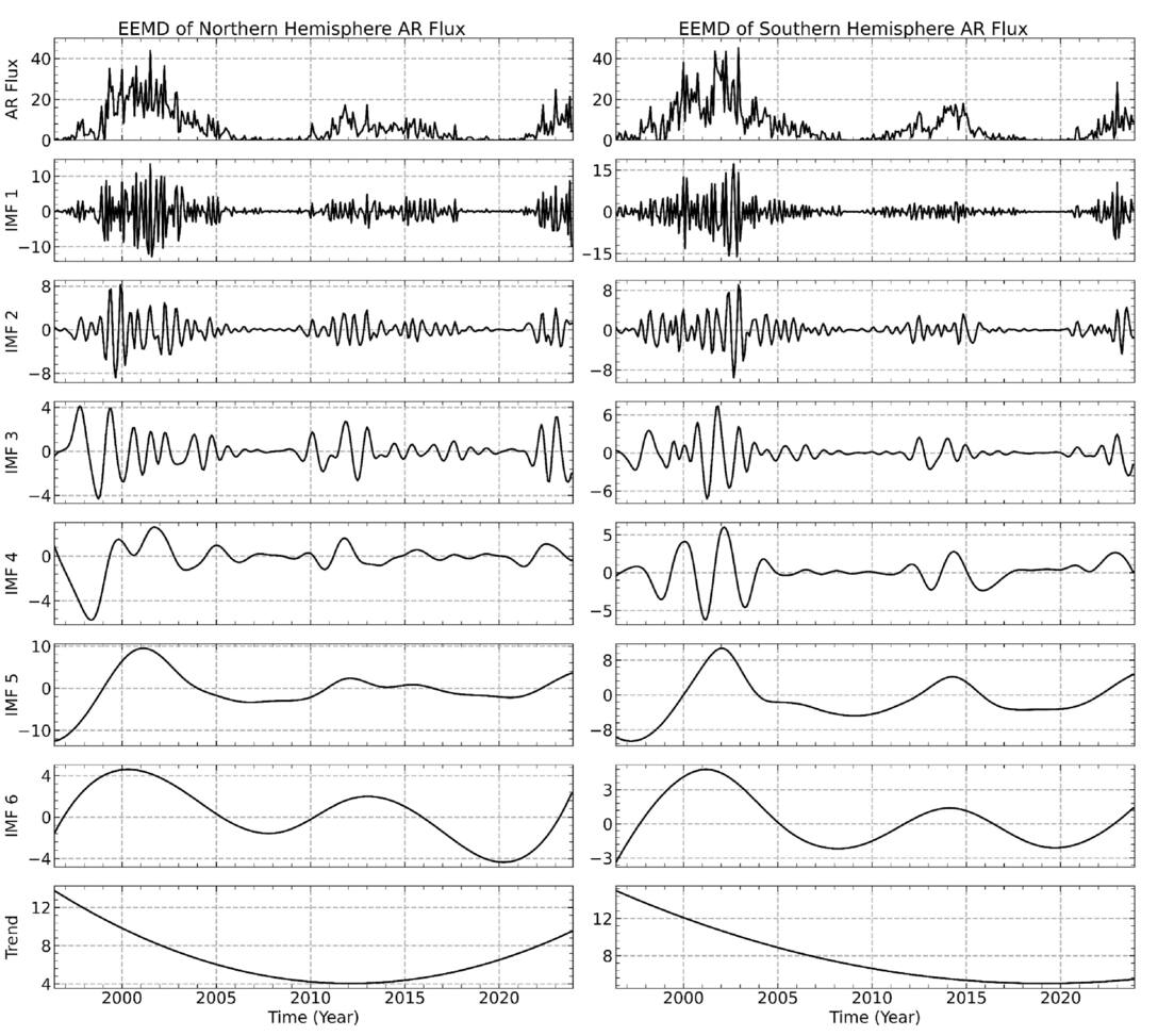
Figure 12. Top panel: monthly values of solar AR flux (1022 Mx) in the northern and southern hemispheres for the time interval from 1996 May to 2023 November. Other panels show the average IMFs of AR flux (1022 Mx). The panels display IMFs 1–6 and the trend in descending order.
Download figure:
Standard image High-resolution imageThe decomposition results are presented in the lower seven panels of Figure 12, with the left and right panels displaying for the northern and southern hemispheres, respectively. A total of six IMFs and a trend component were obtained, with the period values for each IMF provided in Table 3. As shown in Figure 12 and Table 3, IMF5 and IMF6 in both hemispheres represent the 11 yr Schwabe cycle. The IMF6 of the hemispheric AR flux exhibits smaller errors than that of the full-disk AR flux. Therefore, the IMF6 obtained from the flux of the northern and southern hemispheres is considered to represent the 11 yr Schwabe cycle.
Table 3. Average Periodicities of the Six IMFs Derived from the AR Flux for Both Hemispheres
| Northern Hemispheres | Southern Hemispheres | |
|---|---|---|
| (year) | (year) | |
| IMF1 | 0.252 ± 0.001 | 0.208 ± 0.001 |
| IMF2 | 0.537 ± 0.004 | 0.567 ± 0.007 |
| IMF3 | 1.486 ± 0.027 | 1.158 ± 0.122 |
| IMF4 | 2.667 ± 0.087 | 2.292 ± 0.021 |
| IMF5 | 11.333 ± 1.839 | 10.625 ± 0.201 |
| IMF6 | 12.792 ± 0.225 | 11.958 ± 0.199 |
Download table as: ASCIITypeset image
Furthermore, IMF3 and IMF4 correspond to periodicities of 1.486 ± 0.027 yr and 2.667 ± 0.087 yr in the northern hemisphere, and 1.158 ± 0.122 yr and 2.292 ± 0.021 yr in the southern hemisphere. These periods fall within the 1–3 yr timescale and can be considered as the solar QBOs. This suggests that the solar QBOs exist not only in the basic parameters of different ARs but also in the flux of ARs in both hemispheres. Similar to the results obtained from different AR parameters and sunspot numbers, IMF2 is identified as the Rieger-type periodicity, while IMF1 may be attributed to high-frequency noise.
In summary, the periodic modes of the flux of ARs in both hemispheres primarily include the 11 yr Schwabe cycle, the solar QBOs, and the Rieger-type periodicity. These findings align closely with the periodic variations revealed in data analysis of full-disk ARs, demonstrating the consistency and universality of these periodicities across different spatial scales.
3.6.2. Phase Relationships of Hemispheric AR Periodicities
The upper panel of Figure 13 displays time series of ARs in the northern and southern hemispheres at different timescales, where the blue solid line and the red solid line represent the northern and southern hemispheres, respectively. IMF3 and IMF4 are considered as the solar QBOs; Figure 13(b) is obtained by summing the modes of IMF3 and IMF4, while Figure 13(c) is obtained by superimposing IMF5 and IMF6, which is considered to give the 11 yr Schwabe cycle. From the upper panel, it can be seen that within the considered time interval, the periodic variations of ARs at different timescales in the two hemispheres do not occur simultaneously, indicating that the timescale variations in the ARs are not synchronized between the northern and southern hemispheres.
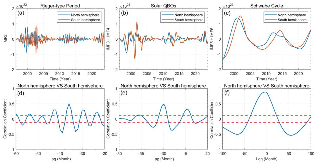
Figure 13. Upper panels: time series of AR flux at different timescales in the northern and southern hemispheres, from left to right representing the Rieger-type periodicity, QBOs, and the Schwabe cycle. Lower panels: CCA results of the periodicities at different timescales for AR flux in the two hemispheres, with the red dashed line indicating the 95% confidence level.
Download figure:
Standard image High-resolution imageThe CCA was employed to examine the phase relationships of periodicities in ARs between the two hemispheres at different timescales. The results are shown in the lower panels of Figure 13. The abscissa represents the phase lag of the northern hemisphere relative to the southern hemisphere, where negative values indicate that the northern hemisphere leads the southern hemisphere, while positive values indicate the opposite. The red dashed line denotes the 95% confidence level.
Figure 13(d) illustrates the phase lag relationship of the Rieger-type periodicity between the two hemispheres. Within the range of −80 to −20 months, the maximum CC of 0.503 occurs at a phase lag of −36 months. Globally, hemispheric Rieger-type periodicity exhibits a positive correlation, but the northern hemisphere peaks 36 months earlier than the southern hemisphere. The phase relationship of the solar QBOs in ARs between the two hemispheres is shown in Figure 13(e). The phase lag between the hemispheres for the solar QBOs is 30 months, with the maximum CC of 0.483 occurring at a lag of −30 months. That is, during the considered time interval, the QBOs of ARs in the northern hemisphere peaks lead the southern hemisphere by 30 months. Figure 13(f) presents the CCA results for the Schwabe cycle between the two hemispheres, with phase lags ranging from −100 to 100 months. The maximum CC is 0.887, corresponding to a phase lag of 4 months, indicating that the Schwabe cycle of ARs in the northern hemisphere peaks 4 months earlier than in the southern hemisphere.
From Figure 13, it is evident that within the considered time interval, the periodic behavior of the AR flux at different times shows differences between the two hemispheres, indicating that the AR flux in the two hemispheres is slightly decoupled. By comparing the hemispheric distribution of the ARs at different timescales, it is found that the ARs exhibit complex phase relationships at different timescales between the two hemispheres. Although the spatial distributions of the Rieger-type periodicity, solar QBOs, and the 11 yr Schwabe cycle differ between the hemispheres, the overall pattern indicates that the AR flux in the northern hemisphere generally peaks earlier than that in the southern hemisphere.
4. Conclusion and Discussion
The investigation of the periodic variations in the AR parameters and the hemispheric asymmetry is crucial for understanding and developing solar dynamo models, as well as for assessing their impact on space weather and Earth’s climate. In this study, we analyzed the multiscale periodic behavior present in the three parameters of the AR flux, area, and number, as well as in the sunspot number, for the period from 1996 May to 2023 November. In particular, we focus on a more in-depth study of the solar QBOs present in these data, including an analysis of the phase relationships of different periodicities in these data and the relationship between the solar QBOs and the 11 yr Schwabe cycle. First, we used the EEMD to decompose four consecutive time series of data consisting of the AR parameters and the sunspot number, with the aim of extracting the underlying periodic patterns present in them. Next, the CCA was used to perform pairwise analysis of AR flux, area, number, and sunspot number, analyzing the Rieger-type period, solar QBOs, and the 11 yr Schwabe cycle separately. Moreover, in order to deepen our understanding of the relationship between the 11 yr Schwabe cycle and the QBOs, the two periodic modes are superimposed, unveiling the Gnevyshev gap phenomenon. Finally, we extract the IMFs of the AR flux in the northern and southern hemispheres, revealing its periodicity and analyzing the phase asynchronism of different periodicities between the two hemispheres.
According to the EEMD technique, the monthly data of AR flux, area, number, and sunspot number were decomposed into six IMFs and one trend component. The typical periodic modes identified in the four data sets mainly include the 11 yr Schwabe cycle, the Rieger-type period, and solar QBOs. Similar periodicities have also been found and reported in other solar activity indices. The detected periodicities in the four time series show differences, indicating that there are similar modulations among the AR flux, area, number, and the sunspot number, but their physical characteristics are distinct. It is worth noting that through a comparative analysis of the solar QBO components during Solar Cycles 23 and 24, it was found that IMF3 and IMF4 exist in both solar cycles. However, it was observed that the solar QBOs represented by IMF3 exhibit more complex periodicity in Solar Cycle 23 than in Cycle 24. This difference may be attributed to changes in the differential rotation in the solar interior during different solar cycles (D. H. Hathaway et al. 2022).
By using the CCA method, we analyzed the phase relationship for the Rieger-type period (IMF2), and the results show that the CC between AR flux and AR area is the highest, while the CC between AR parameters and sunspot number is relatively low. Additionally, we found that the phase relationship of the solar QBOs, when combining IMF3 and IMF4, is complex between different AR parameters and sunspot numbers, with no clear patterns. However, when considering only IMF4, the phase relationship of QBOs between AR flux, area, number, and sunspot number becomes simpler, as the cross-correlograms become smoother. From a global perspective, the solar QBOs of the four parameters are positively correlated. For the 11 yr Schwabe cycle, the four parameters also show a positive correlation, but the CCs for the 11 yr Schwabe cycle are the highest. This suggests that the Rieger-type period, solar QBOs, and the 11 yr Schwabe cycle have different physical origins and variation processes. By comparing the pairwise CCs of the four parameters, we found that the largest CC values between the AR flux and area in different scale periods, indicating that flux and area are more effective in representing changes in ARs. There is a high degree of phase synchronization between the two, which may be the result of the AR flux playing a dominant role (M. Rybanský et al. 2005; P. Li et al. 2014; J. Oloketuyi et al. 2024). F. Li et al. (2024) concluded that the strength of the AR flux can be roughly quantified by the AR area.
By superimposing the 11 yr Schwabe cycle and the solar QBOs, the Gnevyshev gap is observed. This study suggests that the Gnevyshev gap is the result of the modulation of solar QBOs by the 11 yr Schwabe cycle. A distinct double-peaked structure is observed in the AR flux, area, number, and the sunspot number during Solar Cycles 23 and 24. The asynchronous activity between the hemispheres may also contribute to the appearance of the Gnevyshev gap (L. Svalgaard & Y. Kamide 2013). It is well known that solar activity in the northern and southern hemispheres often occurs asynchronously, and if solar activity peaks in one hemisphere before the other, this may lead to two different peaks in one solar cycle (P. Chowdhury et al. 2019; J. Javaraiah 2022). Furthermore, M. Dikpati et al. (2018) proposed that the energetic interactions between the magnetic fields in the solar tachocline, Rossby waves, and differential rotation could lead to nonlinear quasi-periodicity, which is related to the spiky phenomena observed in solar cycles. Based on this, the periodicity of solar activity in the northern and southern hemispheres is also worth further investigation. Furthermore, B. B. Karak et al. (2018) suggested that the peaks and spikes observed in the solar cycle originate from changes in the Babcock–Leighton process, which involves the generation of polar fields from the decay of tilted bipolar magnetic regions (H. W. Babcock 1961). The formation of polar fields in this process is accompanied by a significant negative deviation, which suddenly reduces the total polar field. When the deviation shifts to subsequent ring magnetic fields, it may result in the formation of peaks and spikes (V. N. Obridko et al. 2024). G. A. Bazilevskaya et al. (2000) found that during the maximum phases of Solar Cycles 21 and 22, the amplitude of the QBOs depends on the phase of the 11 yr Schwabe cycle, with QBOs reaching its maximum at the maximum of the solar cycle, which explains the double-peaked structure observed during the solar maximum phase. We hope that in the near future, more observational data sets will be available to drive numerical simulations to better understand and reveal the physical processes underlying the phase of solar QBOs and its relationship with the 11 yr Schwabe cycle.
The issue of the hemispheric asymmetry in solar magnetic activity on different timescales has been discussed by many studies based on solar dynamo theories. D. Shukuya & K. Kusano (2017) studied the interaction between the dipole and quadrupole components of the solar magnetic field and proposed the existence of two different attractors in the solar cycle to explain the asymmetry of polar magnetic field reversal and the phase asymmetry of solar activity. M. Schüssler & R. H. Cameron (2018) used an updated Babcock–Leighton dynamo model and found that the north–south asymmetry of solar magnetic activity can be viewed as a result of the superposition of dipole and quadrupole modes. Additionally, differences in meridional flow velocity and the instability of magnetic Rossby waves may also contribute to the periodic asymmetry observed between the two hemispheres (B. Belucz et al. 2015; J. Shetye et al. 2015; E. Gurgenashvili et al. 2017). However, the exact physical mechanisms that induce this asymmetry still require further investigation. Future studies combining long-term observational data with high-resolution numerical simulations could provide deeper insights into the underlying physical mechanisms.
Acknowledgments
We thank Ruihui Wang, Jie Jiang, and Yukun Luo for creating the homogeneous database of solar active regions. The sunspot data are obtained from the WDC-SILSO, Royal Observatory of Belgium, Brussels. This work is supported by the National Natural Science Foundation of China (12463009), the Yunnan Fundamental Research Projects (grant Nos. 202301AV070007, 202401AU070026, 202501AT070366, 202501AU070154), the “Yunnan Revitalization Talent Support Program” Innovation Team Project (grant No. 202405AS350012), the Scientific Research Foundation Project of Yunnan Education Department (2023J0624, 2024Y469, 2025Y0720, 2025Y0721, 2025J0502), and the GHfund A (202407016295).
Facilities: SOHO - Solar Heliospheric Observatory satellite (MDI), SDO - Solar Dynamics Observatory (HMI - ).
Footnotes
- 8
- 9
- 10