The following article is Free article

Constraining First Star Formation with 21 cm Cosmology

Anna T. P. Schauer, Boyuan Liu, and Volker Bromm

Published 2019 May 16 • © 2019. The American Astronomical Society. All rights reserved.
The Astrophysical Journal Letters, Volume 877, Number 1Citation Anna T. P. Schauer et al 2019 ApJL 877 L5DOI 10.3847/2041-8213/ab1e51

PDF Opens in a new tab.

ePub

You need an eReader or compatible software to experience the benefits of the ePub3 file format.

Article metrics

994 Total downloads
0 Video abstract views

Permissions

Get permission to re-use this article

Dates

Received 2019 January 10
Revised 2019 April 16
Accepted 2019 May 1
Published 2019 May 16

Keywords

dark ages, reionization, first stars; early universe; stars: Population III

Journal RSS

Create or edit your corridor alerts

What are corridors?

Abstract

Within standard ΛCDM cosmology, Population III star formation in minihalos of mass M_halo ≳ 5 × 10⁵M_⊙ provides the first stellar sources of Lyα photons. The Experiment to Detect the Global Epoch of Reionization Signature (EDGES) has measured a strong absorption signal of the redshifted 21 cm radiation from neutral hydrogen at z ≈ 17, requiring efficient formation of massive stars before then. In this Letter, we investigate whether star formation in minihalos plays a significant role in establishing the early Lyα background required to produce the EDGES absorption feature. We find that Population III stars are important in providing the necessary Lyα-flux at high redshifts, and derive a best-fitting average Population III stellar mass of ∼750 M_⊙ per minihalo, corresponding to a star formation efficiency of 0.1%. Furthermore, it is important to include baryon-dark matter streaming velocities in the calculation, to limit the efficiency of Population III star formation in minihalos. Without this effect, the cosmic dawn coupling between 21 cm spin temperature and that of the gas would occur at redshifts higher than what is implied by EDGES.

Export citation and abstractBibTeX RIS

Previous article in issue

Next article in issue

1. Introduction

The recent detection of a 21 cm signal at high redshift has opened a new window for astrophysics at the dawn of star formation (Furlanetto et al. 2006; Pritchard & Loeb 2012). The Experiment to Detect the Global Epoch of Reionization Signature (EDGES) has measured a strong, global (sky-averaged) absorption signal centered around 78 MHz (Bowman et al. 2018). The absorption signal is broad, and a factor of about three stronger than expected within standard ΛCDM, where dark matter only interacts gravitationally. If verified, that signal points to new dark matter physics (e.g., Barkana 2018; Fialkov et al. 2018; Muñoz & Loeb 2018; Slatyer & Wu 2018) or an additional radio background (Ewall-Wice et al. 2018; Feng & Holder 2018).

In this study, we focus on a second characteristic, the implied timing of early star formation. The absorption signal starts at z ≈ 20 and is strongest at z ≈ 17, indicating that at that time the spin temperature of neutral hydrogen is tightly coupled to the gas temperature.

This coupling is mediated through Lyα-radiation via the Wouthuysen–Field effect (Wouthuysen 1952; Field 1958). The critical Lyα background intensity required for effective coupling has been estimated to be 1.8 × 10⁻²¹ [(1 + z)/20] erg s⁻¹ cm⁻² Hz⁻¹ sr⁻¹ (Madau et al. 1997; Ciardi & Madau 2003). Population III stars are typically more massive and therefore hotter than standard populations, resulting in an increased Lyα luminosity (Bromm 2013; Glover 2013). The role of X-ray sources in shaping the thermal history of the early intergalactic medium is still uncertain (e.g., Jeon et al. 2014, 2015), and we thus neglect their contribution in this study.

The Lyα flux emitted from the first galaxies has been studied before in the context of EDGES, requiring large star formation efficiencies (SFEs) to allow strong coupling before redshift z ≃ 17 (e.g., Madau 2018; Mirocha & Furlanetto 2019). Here, we test whether Population III stars in minihalos significantly contribute to the overall Lyα luminosity, and whether the combined star formation activity at high z can provide the necessary photon flux at the right time. Our analysis also provides an upper limit on the overall Population III SFE, as star formation cannot occur too early.

We further include a crucial large-scale effect that influences Population III star formation in minihalos, the relative motion between the cosmic baryon, and dark matter components. These streaming velocities date back to the epoch of recombination (Tseliakhovich & Hirata 2010), described by a multivariate Gaussian spatial distribution with a standard deviation of σ_rms = 30 km s⁻¹. The initially supersonic motion can be assumed to be coherent over large (Mpc) scales, decaying as the universe is expanding. One key effect is the reduced baryon fraction in halos located within regions with streaming velocities, which subsequently leads to a reduced halo mass function (e.g., Naoz et al. 2012; Fialkov 2014). As a result, star formation in such regions is delayed (e.g., Greif et al. 2011; Stacy et al. 2011; Naoz et al. 2013; Hirano et al. 2018; Schauer et al. 2019), and the halo mass necessary for Population III star formation increases. When estimating the star formation rate and Lyα-background flux, we include these effects in our modeling.

2. Methodology

From recent simulations (Schauer et al. 2019), we know the average minihalo mass M_ave necessary for star formation, depending on the halo’s streaming environment. Using the Sheth–Torman mass function (Sheth et al. 2001), we then estimate the respective number of halos that have crossed the mass threshold for star formation. With streaming motions distributed according to a three-dimensional Gaussian (Tseliakhovich & Hirata 2010), we can calculate the fraction of the universe exposed to a given streaming velocity. Convolving these results, we arrive at an estimate for the number density of star-forming halos, as a function of mass and redshift.

In a second step, we parameterize the SFE for these sources, distinguishing between a Population III and Population II stellar component, as the first, metal-free stars are more massive and therefore more luminous (e.g., Bromm 2013; Glover 2013). Because star formation in minihalos is very bursty, we assume a one-time star formation event in each Population III host minihalo, and a fixed star formation history in the more massive halos that host Population II stars. Finally, we calculate the Lyα background luminosity, based on the global stellar density. We provide best-fitting, combined Population III/Population II models that match the redshift position of the EDGES signal.

3. Results

3.1. Threshold Masses for Population III Hosts

We base our analysis on minihalos formed in the Schauer et al. (2019) high-resolution cosmological simulations (see also Schauer et al. 2017). The simulations are initialized at redshift z = 200 with Planck parameters (Planck Collaboration et al. 2016), performed with the AREPO code (Springel 2010), including a network of primordial chemistry. To represent different streaming regions, a constant offset velocity is added to the initial conditions, with an amplitude of 0, 1, 2 and 3σ_rms (v0, v1, v2, and v3). For the 3σ_rms case, a bigger box with four times longer side length is also run (v3_big).

In Figure 1, we illustrate the different effects of streaming velocities. Specifically, in the left panel we show the minimum and average halo masses for the corresponding gas to become cold and dense in the center, and hence eligible for star formation, as a function of streaming velocity. Schauer et al. (2019) did not see any evolution in the minimum or average halo mass, and we employ their redshift-independent threshold values. In the following, we work with the average halo mass, above which more than 50% of all halos are star-forming.

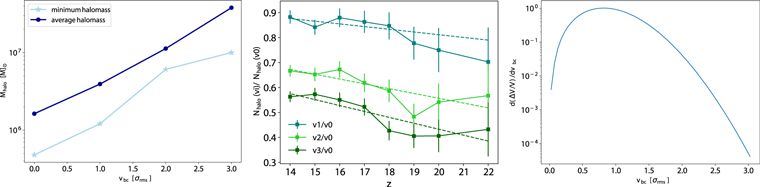
Figure 1. Refer to the following caption and surrounding text. — **Figure 1.** Effects of streaming motion. Left panel: minimum (light blue stars) and average (dark blue dots) halo mass for star formation in minihalos, as a function of streaming velocity (independent of redshift), based on Schauer et al. (2019), for their v0, v1, v2, v3_big simulations. Middle panel: relative number of halos for different streaming velocities, as a function of z, considering all halos with masses larger than M_halo ≥ 4.8 × 10⁵ M_⊙. The solid lines show the raw data, and the dashed lines our redshift dependent linear fits. Right panel: volume fraction as a function of streaming velocity, in units of σ_rms (independent of redshift).
Download figure:
Standard image High-resolution image

3.2. Halo Number Densities

We utilize the halo mass function python tool hmf (Murray et al. 2013) to derive the halo number density for star-forming minihalos, N(M ≥ M_ave), as a function of redshift and halo mass, with the same Planck Collaboration et al. (2016) cosmological parameters as Schauer et al. (2019). We chose the Sheth–Torman mass function,² which is generally thought to fit better at high redshifts (Reed et al. 2007).³ As evident in the middle panel of Figure 1, the halo mass function is reduced in regions with streaming velocity. Specifically, we show the fraction of the mass functions in streaming regions (vi), relative to the no-streaming (v0) case, considering all halos with M_halo ≥ 4.8 × 10⁵ M_⊙. This mass limit corresponds to the minimum halo mass for star formation in the v0 simulation. The halo number is only slightly reduced in simulation v1, but significantly so, at the 50% level, in simulations v2 and v3. At higher redshifts, we have less data to sample as fewer halos have exceeded the mass threshold, resulting in larger error bars.

To estimate how common the streaming regions are, we derive their respective volume filling fractions (e.g., Tseliakhovich et al. 2011; Greif et al. 2011; Fialkov 2014). The velocity distribution follows a multivariate Gaussian:

Integrating P_vbc to infinity, one can derive the fraction of the volume with v_bc or higher. E.g., regions with streaming velocities of 2.0 σ_rms or higher make up less than one percent of the cosmic volume. In the right panel of Figure 1, we present the differential volume fraction, which peaks around 0.8σ_rms. We note that regions with very small streaming velocity are not common.

We present the results for the mass function of star-forming minihalos in Figure 2, with values given in comoving units. In the lower panel, we show the differential halo mass function for different streaming regions at redshift z = 20. For a given streaming velocity, we apply the corresponding minimum mass cut (shown by the blue dots), and multiply with the respective volume filling fraction for an interval v_bc − Δv_bc to v_bc + Δv_bc. A volume filling fraction of 99% corresponds to a mass threshold of 2.1 × 10⁶ M_⊙. The black lines represent the resulting differential mass functions in that streaming region, and their sum equals the volume-averaged halo mass function, as shown in the middle panel. One can see that the contribution to the mass function is largest around v_bc ≈ 1σ_rms. Combining these results, we derive the cumulative halo mass function for star-forming minihalos, averaged over the various streaming regions, shown in the upper panel of Figure 2 for redshifts z = 15, 20 and 30. When accounting for streaming velocities, we find up to one order of magnitude fewer Population III star-forming minihalos, with a comparable effect on the high-z Lyα background flux. It is therefore important to include the impact of streaming motions in any realistic modeling.

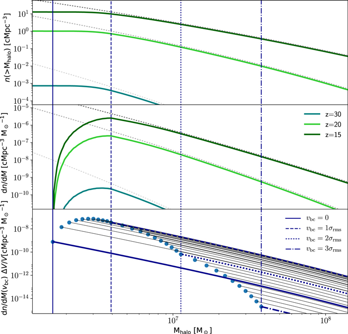
Figure 2. Refer to the following caption and surrounding text. — **Figure 2.** Halo mass function. Upper panel: volume-averaged cumulative mass functions for star-forming minihalos for z = 30 (turquoise), z = 20 (green), and z = 15 (dark green), weighted by the volume fraction of different streaming velocity regions. Middle panel: differential mass function for star-forming minihalos for the same redshifts. In the upper two panels, the gray dotted lines show the situation without streaming velocities. Lower panel: mass functions for star-forming minihalos for small intervals around v_bc, with Δ v_bc = 0. 1σ_rms, evaluated at z = 20. Select velocities are highlighted with the dark blue lines. In all three panels, the vertical lines show the halo mass limit for star formation for the v0 (solid line), v1 (dashed line), v2 (dotted line), and v3 (dashed–dotted line) cases.
Download figure:
Standard image High-resolution image

3.3. Star Formation Models

Star formation at high redshift is typically very bursty. After the first stars have formed in a minihalo, their feedback can prevent further star formation until the halo has grown to higher masses and new gas has fallen in (e.g., Pawlik et al. 2013). For higher mass halos, however, continuous star formation is possible, from gas that is already metal-enriched.

To mimic this dependence on halo mass, we apply a mass threshold, where bursty Population III star formation transitions to a near-continuous mode. We here make the implicit assumption of instantaneous star formation once the mass threshold is crossed. Pawlik et al. (2013) have found in their simulations that the transition in star formation mode occurs at ${M}_{\mathrm{halo}}^{\mathrm{thres}}\approx 1\,\times \,{10}^{8}\,{M}_{\odot }$ , and we adopt this value, for simplicity assumed to be redshift-independent. We summarize our model in Table 1, where SFEs are free parameters. In addition, we consider a comparison model without streaming velocities. We calculate the total physical star formation rate density (SFRD), ${\dot{\rho }}_{\star }$ , as a combination of the Population III and Population II components:

where f_b = Ω_b/Ω₀ = 0.16 is the halo gas fraction, assumed to be equal to the global baryon fraction.

Table 1. Star Formation Parameters

Model	M_halo	SFE	${\dot{N}}_{\mathrm{ion}}$	t_⋆
Population III	M_ave < M_halo < 1 × 10⁸ M_⊙	${M}_{\star }^{\mathrm{III}}$ per halo	10⁴⁸ s⁻¹ M_⊙⁻¹	3 Myr
Population II	M_halo > 1 × 10⁸ M_⊙	$\mathrm{SFE}={M}_{\star }^{\mathrm{II}}/{M}_{\mathrm{gas}}$	10⁴⁷ s⁻¹ M_⊙⁻¹	10 Myr

Note. ${M}_{\star }^{\mathrm{III}/\mathrm{II}}$ is the total stellar mass in Population III/II, and t_⋆ the typical lifetime of massive stars.

Download table as: ASCII Typeset image

Our results are presented in Figure 3, with (comoving) star formation rate densities shown in the middle panel. We choose values of 100 and 1000 M_⊙, as well as our later-determined best-fit model with ∼800 M_⊙ in Population III stars formed in a minihalo, and Population II SFEs of 1% and 5%. One can see that Population III stars initially dominate, with Population II star formation becoming important after z ≈ 20. Neglecting streaming velocities (dotted–dashed lines) leads to unphysically high values.

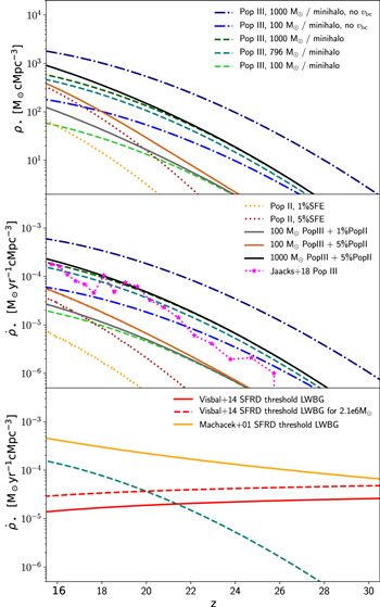
Figure 3. Refer to the following caption and surrounding text. — **Figure 3.** Upper panel: comoving density in massive stars as a function of redshift. Middle panel: comoving SFRD. We show the results for a Population III component (dashed lines) and a Population II component (dotted lines) alone, as well as the combined models (solid lines). The dotted–dashed lines show Population III models when neglecting streaming velocities. The magenta line shows the SFRD from Jaacks et al. (2018) for comparison. Lower panel: comoving SFRD above which a Lyman–Werner background (LWBG) provides the stronger constraints on the minimum halo mass.
Download figure:
Standard image High-resolution image

In the lower panel, we assess at which star formation rate densities the mass threshold dependent on a Lyman–Werner background (LWBG) becomes more strict than our halo mass threshold. Hereby, we convert the SFRD to a LW flux based on a calculation by Johnson (2013). Then we derive the halo mass threshold for star formation based on the LWBG flux with two literature models from Machacek et al. (2001) and Visbal et al. (2014). In this way, for any given SFRD, we can calculate the mass threshold set by the corresponding LWBG, and evaluate whether the effect of a LWBG is dominant by comparing the LWBG-based mass thresholds with those dictated by streaming velocities. We chose the mass thresholds of 1.6 × 10⁶ M_⊙ and 2.1 × 10⁶ M_⊙ to compare with, corresponding to our minimum halo mass for 100% and 99% of the volume of the universe (based on the streaming velocity distribution). One can see that our fiducial model lies below the Machacek et al. (2001) SFRD threshold at all times, and that the LWBG constraint from Visbal et al. (2014) only takes over at redshifts z < 20 for a volume fraction of 99%. When considering streaming velocities, an additional LWBG does not change the SFRD at these high redshifts.

The corresponding total (comoving) mass densities in massive stars can be obtained by integrating over the stellar lifetime (see Table 1), shown in the upper panel of Figure 3. As massive Population II stars have ∼3 times longer lifetimes, their contribution to the total stellar density is a factor of ∼3 higher, compared to the SFRD.

3.4. Lyα Background Flux

The Lyα background intensity can be calculated by integrating over the photon sources in a cosmological volume large enough to allow photons to redshift into the Lyα line. For simplicity, we include all photons between the Lyα resonance and the hydrogen ionization limit, resulting in (1 + z_max)/(1 + z) = 4/3. We further assume a pure blackbody and use effective temperatures corresponding to the ionizing photon numbers for Population III and Population II stars (see Table 1). Following Ciardi & Madau (2003), the Lyα background intensity from Population III stars is then

The proper specific intensity j_ν(z′) can be derived from the spectral energy distribution and the proper stellar mass density:

where the luminosity can be approximated by the Eddington limit L ≈ L_Edd = 1.25 × 10³⁸ erg s⁻¹(M/M_⊙) (Bromm et al. 2001), σ_B is the Stefan–Boltzmann constant, T the effective temperature of the blackbody, and B_ν(T, z′) is the Planck function. ρ_⋆(z′) is the proper stellar density of all Population III stars that have not exceeded their lifetime. The calculation for ${J}_{\alpha }^{\mathrm{II}}$ follows analogously.

The EDGES result implies that the spin temperature of neutral hydrogen needs to be efficiently coupled to the kinetic gas temperature for z ≲ 20. This can be achieved when the thermalization rate due to Lyα scattering is stronger than the coupling between the spin temperature and the cosmic microwave background. Evaluating this condition, Ciardi & Madau (2003) found that J_α ≳ 9 × 10⁻²³(1 + z) erg s⁻¹ cm⁻² Hz⁻¹ sr⁻¹ is required, and we use their estimate in our analysis (see Figure 4).

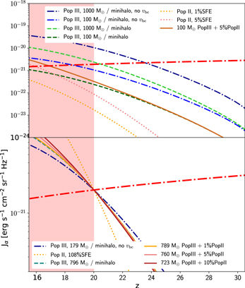
Figure 4. Refer to the following caption and surrounding text. — **Figure 4.** Lyα flux as a function of redshift for our different models. Line styles and colors in the upper panel are the same as in Figure 3. In the lower panel, we show our best-fit models for a Population II component alone (dotted orange line), a Population III component alone (dashed green line), a Population III component that neglects streaming velocities (blue dotted–dashed line), and best-fit models with a Population II SFE of 1%, 5%, and 10% in combination with a Population III component (solid lines). The red dotted–dashed line shows the Lyα flux necessary for effective coupling (from Ciardi & Madau 2003). The shaded red area on the left represents the EDGES timing constraint.
Download figure:
Standard image High-resolution image

In the lower panel of Figure 4, we show the best-fit models. For a Population II component alone, we would require an unphysical SFE of >100%. We thus conclude that Population III star formation is crucial in this context and should not be neglected. Alternatively, Mirocha & Furlanetto (2019), who do not include minihalos, have to assume a steepening of the ultraviolet luminosity function at high redshifts. It is also important to include a treatment of streaming velocities, as one would otherwise predict efficient Wouthuysen–Field coupling too early in cosmic history, which would be incompatible with the EDGES timing constraint. If we consider a combined Population III/II model with a plausible Population II SFE (less than 10%), we infer a best-fit average value of ∼750 M_⊙ in Population III stars per minihalo (solid lines in Figure 4). This corresponds to an average SFE of 0.1% for the streaming velocity averaged halo mass of 4.4 × 10⁶ M_⊙.

4. Conclusions

We have shown with an idealized, semi-analytic model that Population III stars are crucial for establishing a strong Lyα flux early in cosmic history, which in turn can couple the spin temperature to the gas. While we include a detailed treatment of streaming velocities, we make a number of simplifying assumptions. Our study does not address the absorption depth, in the context of interacting dark matter (Barkana 2018). Such interacting dark matter could prevent halo formation at high redshift, or heat the gas in halos with streaming motion between dark matter and baryons (e.g., Hirano & Bromm 2018).

In our analysis of the Population III stellar component, we do not include Lyman–Werner radiation, which can delay the formation of the first stars, thus having similar consequences as streaming velocities (e.g., Machacek et al. 2001; Safranek-Shrader et al. 2012). However, an exploratory analysis has shown that streaming velocities impose the tighter constraints on 99% of all minihalos in our fiducial model. The interplay of Lyman–Werner radiation and streaming velocities is not yet known, and we plan to update our analysis once quantitative estimates are available. Our calculation assumes a top-heavy initial mass function (IMF) for Population III, resulting in a higher effective temperature and thus a higher photon flux than the Population II counterpart. However, the lifetime of Population III stars is a factor of ∼3 smaller than for massive Population II stars, thus leading to a three-times smaller aggregate production of Lyα-photons per stellar baryon. However, even with this factor of three, the Population II SFE would still exceed >30%. A top-heavy IMF is thus not necessarily required to explain the EDGES signal, but a high-z contribution from minihalos is. Streaming velocities suppress star formation in low-mass halos, and therefore increase the required average stellar mass per minihalo by a factor of ∼5. Furthermore, our results disfavor dark matter models, which aggressively suppress the formation of small-scale structures, such as axion-like ultralight dark matter (Sullivan et al. 2018), or some warm dark matter scenarios (Dayal et al. 2017; Safarzadeh et al. 2018). 21 cm cosmology clearly has tremendous potential to enhance our understanding of how primordial stars transformed the early universe.

We would like to thank Aaron Smith and the anonymous referee for their helpful comments. Support for this work was provided by NASA through the Hubble Fellowship grant HST-HF2-51418.001-A, awarded by STScI, which is operated by AURA, under contract NAS5-26555. V.B. was supported by the National Science Foundation (NSF) grant AST-1413501. The authors gratefully acknowledge the Gauss Center for Supercomputing for providing resources on SuperMUC at the Leibniz Supercomputing Center under projects pr92za and pr74nu.

Footnotes

2
We have verified that our main conclusions do not change for a Press–Schechter function.
3
We chose to work in this semi-analytical framework, as fitting functions from simulations depend on the cosmology and are rare at high redshifts (see Trac et al. 2015, for a WMAP cosmology).

Please wait… references are loading.

Constraining First Star Formation with 21 cm Cosmology

Authors

Author notes

Notes